Laboratoire d'Analyse et Modélisation de Systèmes pour
l'Aide à la Décision
CNRS UMR 7243CAHIER DU LAMSADE
310
Mai 2011
On Multiprocessor Temperature-Aware
Scheduling Problems
Evripidis Bampis, Dimitrios Letsios, Giorgio Lucarelli,
Evangelos Markakis and Ioannis Milis
On Multiprocessor Temperature-Aware
Scheduling Problems
Evripidis Bampis
∗†LIP6, Universit´e Pierre et Marie Curie, France [email protected]
Dimitrios Letsios
IBISC, Universit´e d’ ´Evry, France [email protected]
Giorgio Lucarelli
∗LAMSADE, Universit´e Paris-Dauphine, France [email protected]
Evangelos Markakis and Ioannis Milis
Dept. of Informatics, Athens University of Economics and Business, Greece {markakis,milis}@aueb.gr
Abstract
We study temperature-aware scheduling problems under the model introduced by Chrobak et al. in [6]. We consider a set of parallel identi-cal processors and three optimization criteria: makespan, maximum tem-perature and (weighted) average temtem-perature. On the positive side, we present polynomial time approximation algorithms for the minimization of the makespan and the maximum temperature, as well as, optimal poly-nomial time algorithms for minimizing the average temperature and the weighted average temperature. On the negative side, we prove that there is no (43 − ϵ)-approximation algorithm for the problem of minimizing the makespan for any ϵ > 0, unlessP = N P.
1
Introduction
The exponential increase in the processing power of recent (micro)processors has led to an analogous increase in the energy consumption of computing systems of any kind, from compact mobile devices to large scale data centers. This has
∗Research supported by the French Agency for Research under the DEFIS program TODO,
ANR-09-EMER-010.
also led to vast heat emissions and high temperatures affecting the processors’ performance and reliability. Moreover, high temperatures reduce the lifetime of chips and may permanently damage the processors. For this reason, man-ufacturers have set appropriate thresholds in processors’ temperature and use cooling systems working almost permanently. However, the energy consump-tion and heat emission of these cooling systems have to be added to that of the whole system.
The issues of the energy and thermal management, in the (micro)processor and system design levels, date back to the first computer systems. During the last few years these issues have been also addressed at the operating system’s level, generating new interesting questions. In this context the operating system has to decide the order in which the jobs should be scheduled so that the system’s temperature (and/or energy consumption) remains as low as possible, while at the same time some standard user or system oriented criterion (e.g. makespan, response time, throughput, etc) is optimized. Clearly, the minimization of the temperature and the optimization of the scheduling criteria are, in general, in conflict. Towards this direction several models have been proposed in the literature. A first model is based on the speed-scaling technique for energy saving and the Newton’s law of cooling; see for example [4, 3] as well as recent reviews on speed scaling in [9, 1, 2]. In another model proposed in [12], a thermal RC circuit is utilized to capture the temperature profile of a processor.
In this paper we adopt the simplified model for cooling and thermal man-agement introduced by Chrobak et al. in [6], which has been motivated by [11]. We consider a set of unit-length jobs (corresponding to slices of the processes to be scheduled), each one of a given heat contribution, and model the thermal behavior of the system as follows: If a job of heat contribution h is executed on a processor in a time interval [t− 1, t), t ∈ N, and the temperature of the processor at time t− 1 is Θ, then the processor’s temperature at time t is Θ+hc , where c is a given cooling factor. We consider two natural variants of the model: - the threshold thermal model in which a given threshold on the temperature of the processors cannot be violated. This makes necessary the introduc-tion of idle times in a schedule.
- the optimization thermal model in which there is no explicit upper bound on the temperature of the processors. The lack of such an explicit bound is counterbalanced by the fact that the minimization of the (maximum or average) temperature becomes the goal of the scheduler.
The constraints that are introduced by such temperature management mod-els give rise to interesting and technically challenging scheduling problems, which is the focus of our work. In particular, our goal is to schedule a set of jobs on a set of m parallel identical processors so as to minimize (i) the makespan in the threshold thermal model and (ii) the maximum or average temperature in the optimization thermal model.
Related results and our contribution. In [6], Chrobak et al. consider the
study the problem of scheduling a set of unit-length jobs with release dates and deadlines on a single processor so as to maximize the throughput, i.e. the number of jobs that meet their deadlines, without exceeding the temperature threshold θ at any time t∈ N. Extending the well-known three-field notation for scheduling problems, this problem is denoted as 1|ri, pi= 1, hi|
∑
Ui. They
prove that this problem is NP-hard even for the special case when all jobs are released at time 0 and their deadlines are equal, i.e. 1|pi= 1, di = d, hi|
∑
Ui.
Furthermore, they study the on-line version of the throughput maximization problem in the presence of release dates and deadlines. They prove that a fam-ily of reasonable list scheduling algorithms, including coolest first and earliest
deadline first algorithms, have a competitive ratio of at most two. In the
neg-ative side, they also give an instance that shows that there is no deterministic on-line algorithm with competitive ratio less than two. This result implies also an approximation factor of two for the off-line problem.
The analysis of the family of reasonable algorithms of [6] is generalized by Birks et al. in [5] for other values of c. In fact, for c > 2 they claim a competitive ratio of 2 and for 1 < c < 2 they give a tight competitive ratio that tends to infinity as c tends to 1. Moreover, they present non-constant competitive ratios for the cases of multiple processors and weighted throughput.
We initiate the study of three additional optimization criteria under the model of [6] and under the optimization thermal model. Furthermore, we study all criteria for the case of multiple processors, unlike [6]. In Section 3 we ad-dress the problem of minimizing the schedule length (makespan) in the threshold thermal model (P|pi = 1, hi, θ|Cmax). We prove that this problem cannot be
approximated within a factor less than 4/3 and we present a 73−3m1 approxi-mation algorithm, where m is the number of processors. For the case of a single processor, this yields a 2 approximation. In Sections 4 and 5 we move to the optimization thermal model. In Section 4, we study the problem of minimizing the maximum temperature of a schedule (P|pi = 1, di = d, hi|Θmax), and we
give a 4/3 approximation algorithm. In Section 5, we prove that the problem of minimizing the average temperature of a schedule (P|pi= 1, di= d, hi|
∑ Θi),
as well as a time-dependent weighted version of this problem are both solvable in polynomial time. In order to avoid trivial solutions for the maximum and average temperature objectives, we assume a given common deadline for all jobs in the instances of these problems (see Section 2). We conclude in Section 6.
2
Notation and Preliminaries
We consider a set J = {J1, J2, . . . , Jn} of n jobs to be executed on a system
of m identical processors. All jobs have unit processing times and for each one of them we are given a heat contribution hi, 1≤ i ≤ n. We consider each job
Ji executed in a time interval [t− 1, t), t ∈ N, which we call (time) slot t, on
some processor. By Θt we denote the temperature of a processor at time t.
executing job Ji at time t− 1, then Θt= Θt−12+hi. The initial temperature of
each processor (the ambient temperature) is considered to be zero, i.e., Θ0= 0.
The threshold thermal model. In this model, the temperature is not al-lowed to exceed a threshold θ at any time t∈ N. It is clear that, for a given instance in this model, a feasible schedule may exist only if hi ≤ 2 · θ for each
job Ji. By normalizing the values of hi’s and θ we can assume w.l.o.g. that
0 < hi ≤ 2 and θ = 1. Moreover, if a processor at time t − 1 has temperature
Θt−1 and it holds that
Θt−1+hi
2 > 1, for every job Ji that has not yet been
scheduled, then this processor will remain idle for the slot [t− 1, t) and its tem-perature at time t will be reduced by half, i.e., Θt−12 . Note also that once a processor has executed some job(s) its temperature will never become exactly zero. Therefore, in this model, a feasible instance can not contain more than m jobs of heat contributions equal to 2, as there are m slots with Θ0= 0 (the first
slots in each one of the m available processors).
The optimization thermal model. In this model, no explicit temperature threshold is given and the problems we will study are the minimization of max-imum and average temperature. For any instance in this model, any schedule of length at least⌈mn⌉ is feasible, independently of the range of the jobs’ heat contributions. However, the optimum value of our objectives depends on the time available to execute the given set of jobs: the maximum or average tem-perature of a schedule of length⌈mn⌉is, clearly, greater than that of a schedule of bigger length, where we are allowed to introduce idle slots. Due to this fact, we introduce in the instances of our problems a common deadline d≥⌈mn⌉for all the jobs and we ask for a schedule that minimizes our objectives within this deadline. For these problems, we also consider only instances with n = m· d, since for instances with n < md we can simply add md− n fictive jobs of heat contribution equal to zero. Thus, the number of jobs equals the total number of available slots of the m processors.
We close this section by elaborating on the complexity of the problems studied in the rest of the paper. It is already mentioned in [6] that even for a single processor, the NP-hardness of the maximum throughput prob-lem for the case where jobs are released at time 0 and all deadlines are equal (1|pi = 1, di = d, hi, θ|
∑
Ui) implies the NP-hardness of the makespan
mini-mization problem (1|pi= 1, hi, θ|Cmax). In fact, the decision version of the
lat-ter problem asks for the existence of a feasible schedule where all jobs complete their execution by some given deadline C. Moreover, the decision version of the maximum temperature problem for a single processor (1|pi= 1, di= d, hi|Θmax)
asks for the existence of a schedule where all jobs complete their execution by some given deadline d without exceeding a given temperature threshold θ. Therefore, the same reduction gives NP-hardness for both makespan and max-imum temperature minimization problems. The NP-hardness for our problems on an arbitrary number of parallel processors follows trivially.
3
Makespan Minimization
In this section we study the makespan minimization under the threshold thermal model, that is P|pi= 1, hi, θ|Cmax.
We start with a negative result on the approximability of our problem. The proof of the next theorem is based on adapting a reduction given in [6] for the complexity of throughput maximization under the same model.
Theorem 1. It is NP-hard to approximate the minimum makespan problem
(P|pi= 1, hi, θ|Cmax) within a factor better than 4/3.
Proof. We give a reduction from Numerical 3-Dimensional Matching (N3DM),
where given three sets A, B, C of n integers each and an integer β, we ask for n triples (a, b, c)∈ A × B × C such that each integer belongs to exactly one triple and a + b + c = β for each triple. Wlog, we assume that ∑x∈A∪B∪Cx = βn
and x≤ β for each x ∈ A ∪ B ∪ C. Given instance of N3DM, we construct an instance of P|pi = 1, hi, θ|Cmax consisting of n processors and 3n jobs, one
for each integer in A∪ B ∪ C. Considering the function f(x) = 251 (
1 +8βx )
, we set h(a) = 8f (a) + 1 for each a∈ A, h(b) = 4f(b) + 1 for each b ∈ B and
h(c) = 2f (c) + 1 for each c∈ C.
The hardness of approximation is obtained by the following claim:
Claim 1. There is a N3DM if and only if there is a feasible schedule for
P|pi= 1, hi, θ|Cmax of length three.
Proof. (⇒) Assume that there is a solution for N3DM. For the i-th triple
(ai, bi, ci), 1 ≤ i ≤ n, in this solution, we schedule in the i-th processor the
jobs corresponding to ai, bi and ci in the first, second and third slots,
respec-tively. For the temperatures, Θai, Θbi, Θci, of the i-th processor after each one
of those executions we have
Θai = 8f (ai)+1 2 ≤ 8f (β)+1 2 = 8 25(1+ β 8β)+1 2 = 34 50 ≤ 1 Θbi = 8f (ai)+1 4 + 4f (bi)+1 2 = 3 4+ 2 ( 1 25 ( 1 + ai 8β ) + 1 25 ( 1 + bi 8β )) ≤ 3 4 + 4 25+ β 100β = 92 100 ≤ 1 Θci = 8f (ai)+1 8 + 4f (bi)+1 4 + 2f (ci)+1 2 = 78 +251 ( 1 + ai 8β ) +251 ( 1 + bi 8β ) +251 ( 1 + ci 8β ) ≤ 7 8+ 3 25+ β 200β = 1
and hence there is a feasible schedule of length three.
(⇐) Assume, now, that there is a feasible schedule of length three. In this schedule there are exactly three jobs in each processor, since there are 3n jobs in total.
If a job corresponding to an integer a∈ A is scheduled to the second slot of a processor, then the temperature threshold θ = 1 is violated after the third slot of this processor. Indeed the temperature at this slot will be at least
2f (0)+1 8 + 8f (0)+1 4 + 2f (0)+1 2 = 7 8+ 1 25 ( 1 +8β0) (28+48+22)=201200 > 1.
In a similar way, we can show that a job corresponding to an integer a ∈ A cannot be scheduled to the third slot of a processor:
2f (0)+1 8 + 2f (0)+1 4 + 8f (0)+1 2 = 7 8+ 1 25 ( 1 +8β0) (28+42+82)=213200 > 1.
Hence, each of the n jobs corresponding to one of the n integers a ∈ A is scheduled to the first slot of a processor. Moreover, we can show that a job corresponding to an integer b ∈ B cannot be scheduled to the third slot of a processor: 8f (0)+1 8 + 2f (0)+1 4 + 4f (0)+1 2 = 7 8+ 1 25 ( 1 +8β0) (88+42+42)=201200 > 1.
In all, in each processor exactly three jobs are scheduled: a job a∈ A in the first slot, a job b∈ B in the second slot, and a job c ∈ C in the third slot. Therefore, the jobs of a processor correspond to a feasible triple for N3DM.
To finish our proof, we have to show that each triple sums up to β. If this does not hold then there is a triple (a, b, c) for which a + b + c > β, since ∑
x∈A∪B∪Cx = βn. The temperature of the third slot of the processor in which
the corresponding jobs to this triple are scheduled is
8f (a)+1 8 + 4f (b)+1 4 + 2f (c)+1 2 = 7 8 + 1 25 ( 3 + a+b+c8β ) > 78+251 ( 3 +8ββ ) > 1,
which is a contradiction that there is a feasible schedule.
This completes the proof of Theorem 1 since an approximation ratio better than 4/3 would be able to decide the N3DM problem.
In what follows in this section, we present an approximation algorithm for the minimum makespan problem. Note that, in order to respect the tempera-ture threshold, a schedule may have to contain idle slots. To argue about the number of idle slots that are needed before the execution of each job, we will introduce first an appropriate partition of the set of jobs according to their heat contribution. In particular, for each k ≥ 0, we can argue separately for jobs whose heat contribution belongs to the interval (22kk−1−1,2
k+1−1
2k ]; recall that
hi ≤ 2, 1 ≤ i ≤ n. Moreover, the interval to which a job of heat contribution
hi belongs to is denoted by ki, that is
ki= max{k | hi> 2
k−1
2k−1}.
Our algorithm is based on the following proposition that bounds the number of idle slots needed before the execution of a job in a feasible schedule.
Proposition 1. Any schedule in which every job Ji is executed after at least ki
idle slots is feasible.
Proof. Let x be the number of idle slots that precede the execution of job Ji and Θ be the temperature of the processor before the first of these slots.
This temperature becomes 2Θx, after the last of these slots, and
Θ 2x+hi
2 after the
execution of job Ji. Such a schedule is feasible if Θ≤ 1 and
Θ 2x+hi
2x ≥ Θ
2−hi. Hence, for Θ = 1 and hi >
2ki−1
2ki−1, it follows that 2
x > 1 2−2ki−1 2ki −1 = 2ki−1, that is x≥ k i.
The algorithm works as follows: it first sorts the jobs in a non-increasing or-der of their heat contributions, h1≥ h2≥ . . . ≥ hn, and schedules the m hottest
of them to the first slot of each processor. Then, each one of the remaining jobs,
Ji, m + 1≤ i ≤ n, is scheduled by leaving before its execution exactly ki idle
slots, according to the Proposition 1. Essentially, our problem, for these n− m coolest jobs, is transformed to an instance of the classical P||Cmax scheduling
where the processing time of such a job, equals the minimum number of idle slots of Proposition 1 plus its original unit processing time, i.e., pi = ki+ 1.
Then, these jobs are scheduled using the standard Longest Processing Time (LPT) rule. The LPT rule simply assigns the next job (in the non-increasing order of their processing times) to the first available processor.
Algorithm MAX C
1: Sort the jobs in non-increasing order of their heat contributions: h1≥ h2≥ ...≥ hn;
2: for i = 1 to m do
3: Schedule job Ji to the first slot of processor i;
4: for i = m + 1 to n do
5: Let pi= ki+ 1 be the processing time of job Ji;
6: Complete the schedule by running LPT for Jm+1, Jm+2, . . . , Jn;
To analyze our Algorithm MAX C, we first need a bound on the optimal makespan. The following proposition provides a lower bound to the number of slots that are required between two jobs, both of heat contributions greater than one, in an optimal schedule.
Proposition 2. In an optimal schedule, between the execution on the same
processor of jobs Jj and Ji of heat contributions hj, hi > 1, there are at least
ki− 1 slots, which are either idle or execute jobs of heat contribution at most
one.
Proof. Let Θt be the temperature of the processor before executing Jj. Next,
after the execution of Jj we have Θt+1 =
Θt+hj
2 . Then, after x slots (idles
or executing jobs of heat contribution h≤ 1) we get a temperature Θt+x+1 ≥
Θt+hj
2 ·
1
2x. In order Ji to be executed in the next slot, it should hold that
Θt+x+1+ hi≤ 2, that is 2x≥ Θt+hj 2(2−hi). Since, Θt≥ 0, hj > 1 and hi> 2ki−1 2ki−1 we get 2x≥ Θt+hj 2(2−hi) > 1 2(2−2ki−1 2ki −1) = 12 2ki −1 = 2ki−2, that is x≥ k i− 1.
In the next lemma we obtain a lower bound on the optimal makespan, de-noted by OP T , by bounding, using the previous proposition, the number of slots required for executing all the jobs.
Lemma 1. For the optimal makespan it holds that OP T ≥ 1 +
∑n
i=m+1(ki+1)
2m ,
where the jobs are indexed in non-increasing order of their heat contributions, i.e., h1≥ h2≥ . . . ≥ hn.
Proof. A first trivial lower bound on the optimal makespan follows by
consider-ing all jobs requirconsider-ing a sconsider-ingle time slot for their execution, that is OP T ≥ mn.
However, this bound is too weak if there are jobs requiring a number of idle slots before their execution accordingly to Proposition 2. To take into account this fact, we obtain a second bound by considering only the jobs of heat contribution hi> 1. Let A be the subset of these jobs assigned to any, but
the first, slot of any processor and L(A) be the length of the optimal schedule for these jobs, that is OP T = 1 + L(A).
By Proposition 2, each job Ji ∈ A, requires at least ki slots to be executed
(one of them for its own execution). As jobs of heat contribution hi ≤ 1 have
ki = 0, it follows that OP T = 1 + L(A)≥ 1 + ∑ Ji∈Aki m ≥ 1 + ∑n i=m+1ki m .
Combining the two bounds given above by the standard average argument we get OP T ≥ m+ ∑n i=m+1ki+n 2m = 1 + ∑n i=m+1(ki+1) 2m .
Theorem 2. Algorithm MAX C achieves an approximation ratio of 73 − 1 3m for the minimum makespan problem.
Proof. Our proof follows the standard analysis given in [8], for the classical
multiprocessor scheduling problem. Note, however, that for each job Ji not
executed in the first slot of any processor, the Algorithm MAX C devotes ki+
1 slots, while the bound of Lemma 1 counts ki slots for such a job of heat
contribution greater than one.
Let Jℓ be the job which finishes last in the schedule provided by Algorithm
MAX C. This job will start executed not later than 1 +
∑n
i=m+1,j̸=ℓ(ki+1)
m , and
hence for the length, C, of the schedule provided by Algorithm MAX C it holds that C≤ 1 + ∑n i=m+1,j̸=ℓ(ki+1) m + (kℓ+ 1) = 1 + ∑n i=m+1(ki+1) m + ( 1−m1)(kℓ+ 1).
Hence, by Lemma 1 we get C≤ 2OP T − 1 +(1−m1)(kℓ+ 1).
If kℓ≤ OP T/3, then the theorem follows directly.
If kℓ > OP T /3, then we consider the subinstance, I′, of the original
prob-lem that contains only the jobs of heat contribution at least hℓ, i.e., J′ =
{J1, J2, . . . , Jℓ}. Obviously, k1 ≥ k2 ≥ . . . ≥ kℓ > OP T3 ≥ 1. Moreover, for
the length of an optimal schedule, OP T (I′), of the subinstance I′ it holds that OP T (I′) ≤ OP T and the lengths of the schedules returned by Algo-rithm MAX C for instances I and I′ are equal, i.e., C(I′) = C. Hence,
C OP T ≤
C(I′)
OP T (I′).
In an optimal schedule of I′ there are at most three jobs in each processor, for otherwise, if there is a processor with four assigned jobs, the length of that
schedule will be, by Proposition 2, at least 1 + 3kℓ > OP T , a contradiction.
Hence, there are at most ℓ≤ 3m jobs in I′.
The Algorithm MAX C schedules the job Ji, 1≤ i ≤ m, to the first slot of
processor i, the job Jm+i, 1≤ i ≤ m, to the second slot of processor i and the
job J2m+i, 1≤ i ≤ ℓ − 2m, to the next available slot of processor m − i + 1.
In this schedule there is at least one processor executing three jobs and hence
C(I′)≥ 1 + 2(kℓ+ 1)≥ 5.
Consider now the Algorithm MAX C running on instance I′, but with pi =
ki (instead of pi = ki+ 1) for each job Ji∈ J′, m≤ i ≤ ℓ. The length of this
schedule, say H, is at most two time slots shorter than C(I′), since at most three jobs are executed in any processor and one of them is assigned to its first slot, that is H(I′)≥ C(I′)− 2.
Consider now the optimal schedule for instance I′. We denote by A⊆ J′ the jobs executed in any, but the first, slot of the m processors and by L(A), the length of this schedule. Since the length of the first part of that schedule does not depend on the jobs in the set I′\ A, i.e., the jobs assigned to the first slot of the m processors, we get OP T (I′) = 1 + L(A)≥ 1 + L(A′), where
A′={Jm+1, Jm+2, . . . Jℓ}. As the jobs in A′are less than 2m, they are scheduled
in H in an optimal way (due to LPT rule) and also using the least possible number of slots according to Proposition 2, that is OP T (I′)≥ H(I′).
Therefore, C OP T ≤ C(I′) OP T (I′) ≤ C(I′) H(I′) ≤ C(I′) C(I′)−2 = 1 + 2 C(I′)−2 ≤ 1 + 2 3 = 5 3,
and the proof is completed.
For the case of a single processor the approximation ratio of Algorithm MAX C becomes equal to two. Moreover, in this case, a stronger result holds.
Theorem 3. Any algorithm which executes the hottest job in an instance of
the 1|pi = 1, hi, θ|Cmax problem, in the first slot of the schedule achieves a 2-approximation ratio.
Proof. For the case of a single processor, the lower bound for the optimal
sched-ule proved in Lemma 1 becomes OP T ≥ 1 +
∑n i=2(ki+1)
2 . Using Proposition 1,
the length, C, of the schedule of an algorithm that executes the hottest job in the first slot is at most 1 +∑ni=2(ki+ 1). Therefore, OP TC ≤
1+∑n i=2(ki+1) 1+ ∑n i=2(ki+1) 2 ≤ 2.
4
Maximum Temperature Minimization
Now, we turn our attention to the optimization thermal model and to the prob-lem of minimizing the maximum temperature, i.e., P|pi = 1, di = d, hi|Θmax.
Recall that as we discussed in Section 2, we consider a common deadline d≥⌈mn⌉ for all jobs and that n = m·d, by adding the appropriate number of fictive jobs. By Θ∗maxwe denote the maximum temperature of an optimal schedule.
We start with the observation that any algorithm for this problem achieves a 2 approximation ratio. Indeed, it holds that Θ∗max≥ hmax/2, no matter how
we schedule the job of maximum heat contribution. It also holds that for any algorithm, Θmax ≤ hmax, with Θmax being the maximum temperature of the
algorithm’s schedule. Therefore, Θmax≤ 2 · Θ∗max.
To improve this trivial ratio we propose the following algorithm which is based on the intuitive idea of alternating the execution of hot and cool jobs.
Algorithm MAX T
1: Sort the jobs in non-increasing order of their heat contributions: h1≥ h2≥ ...≥ hn;
2: Using the order of Step 1, schedule the⌈d2⌉m hottest jobs to the odd slots
of the processors using Round-Robin;
3: Using the reverse order of Step 1, schedule the ⌊d2⌋m coolest jobs to the even slots of the processors using Round-Robin;
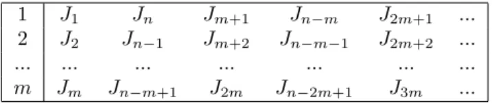
To elaborate a little more on how the algorithm works, note that processor 1 will be assigned the job J1, followed by Jn, then followed by Jm+1, and then
by Jn−m and this alternation of hot and cool jobs will continue till the end of
the schedule. Similarly processor 2 will de assigned the jobs J2, Jn−1, Jm+2,
Jn−m−1, and so on. The schedule is illustrated further in Table 1.
1 J1 Jn Jm+1 Jn−m J2m+1 ...
2 J2 Jn−1 Jm+2 Jn−m−1 J2m+2 ...
... ... ... ... ... ... ...
m Jm Jn−m+1 J2m Jn−2m+1 J3m ...
Table 1: The schedule produced by Algorithm MAX T.
To analyze the Algorithm MAX T, we start with the proposition below, which is implied by the Round-Robin scheduling of jobs in its Steps 2 and 3.
Proposition 3. In the schedule returned by Algorithm MAX T:
(i) A job Ji, i≥
(⌊d
2
⌋
+ 1)m + 1, is succeeded by the job Jn−i+m+1.
(ii) A job Ji, m + 1≤ i ≤
⌈d
2
⌉
m, is preceded by the job Jn−i+m+1.
The maximum temperature may appear at various points of the schedule of Algorithm MAX T. The next lemma states that one of these points satisfies a certain property regarding the heat contribution of the job executed right before.
Lemma 2. In the schedule returned by Algorithm MAX T, the maximum
tem-perature is achieved after the execution of a job Ji, with i≤
(⌊d
2
⌋
+ 1)m. Proof. Assume that all the points where the maximum temperature Θmaxoccurs
are after the execution of a job Ji, with i≥
(⌊d
2
⌋
+ 1)m + 1. By Proposition 3,
returned by Algorithm MAX T. It is easy to check that i > i′, hence hi′ ≥ hi.
Let Θ, Θ′ ≤ Θmax be the temperatures before the execution of Ji and after
the execution of Ji′, respectively. Then, Θmax = Θ+h2 i and hi ≥ Θmax, since
Θmax≥ Θ. Moreover, Θ′ = Θmax2+hi′ ≥ Θmax, since hi′ ≥ hi. This implies that
Θ′ = Θmax, since Θ′ ≤ Θmax. But this means that the maximum temperature
is also achieved after the execution of job Ji′, which is a contradiction because
i′ = n− i + m + 1 ≤ m(d −⌊d2⌋)≤ m(⌊d2⌋+ 1) contrary to what we assumed in the beginning of the proof.
Lemma 3. For the maximum temperature of an optimal schedule it holds that
Θ∗max≥ hn−i+m+1 4 + hi 2, for any i, m + 1≤ i ≤ ⌈d 2 ⌉ m.
Proof. Consider a job Ji and let Ji′ be its previous job in the same processor
in an optimal schedule S∗. The jobs executed in the first slot of each processor in S∗do not have a previous one. To simplify the presentation of our proof, we assume that they are preceded by hypothetical jobs Jn+j, 1≤ j ≤ m.
If i′ ≤ n − i + m + 1, then Θ∗max ≥ hi′ 4 + hi 2 ≥ hn−i+m+1 4 + hi 2, since hi′ ≥ hn−i+m+1.
If i′ > n− i + m + 1, then let B = {Jn−i+m+2, Jn−i+m+3, . . . , Jn, Jn+1,
. . . , Jn+m} and let A be the set of jobs that precede the jobs J1, J2, . . . , Ji−1 in
the optimal schedule. Clearly,|B| = |A| = i − 1, Ji′ ∈ B and Ji′ ∈ A since J/ i′
precedes Ji in S∗.
Therefore, there is a job Jk′ ∈ A such that Jk′ ∈ B, that is k/ ′ < n−i+m+2.
For any i ≤ ⌈d2⌉m, the job Jk′ precedes a job Jk in S∗ and since Jk′ ∈ A it
follows, by the definition of the set A, that k < i. Hence, Θ∗max≥ hk′
4 + hk 2 ≥ hn−i+m+1 4 + hi
2, since hk ≥ hi and hk′ ≥ hn−i+m+1.
Theorem 4. Algorithm MAX T achieves a 43 approximation ratio.
Proof. By Lemma 2 the maximum temperature in the schedule, S, obtained by
Algorithm MAX T occurs after the execution of a job Ji, i≤
(⌊d
2
⌋
+ 1)m (the
maximum may be achieved in other timeslots as well).
If 1≤ i ≤ m, then the maximum occurs at the first processor and Θmax =
h1
2 ≤ Θ∗maxand, hence, the algorithm returns an optimal schedule.
If m + 1 ≤ i ≤ ⌈d2⌉m then by Proposition 3, the job Ji is preceded in
the schedule S by the job Jn−i+m+1. Let Θ be the temperature before the
execution of the job Jn−i+m+1. By Lemma 3, and since Θ ≤ Θmax, Θmax = Θ 4 + hn−i+m+1 4 + hi 2 ≤ Θmax
4 + Θ∗max. Hence, Θmax≤43· Θ∗max.
Note that if d is odd, then⌈d
2
⌉
m =(⌊d
2
⌋
+ 1)m. Hence the only remaining
case is that d is even and ⌈d2⌉m + 1 ≤ i ≤ (⌊d2⌋+ 1)m. For this case, let
Θ′ ≤ Θmax be the temperature before the execution of Ji. Then, hi ≥ Θmax,
since Θmax=Θ
′+h i
2 and Θmax≥ Θ′. Thus, there are at least
⌈d
2
⌉
m + 1 jobs of
heat contribution at least Θmax. Note that, in any schedule, each processor can
execute at most⌈d2⌉jobs without any pair of them scheduled in two consecutive slots. Hence, in an optimal schedule, there are at least two jobs Jp and Jq,
p, q≤ i, executed in consecutive slots in the same processor. Therefore, Θ∗max≥ hp 4 + hq 2 ≥ Θmax 4 + Θmax 2 = 3
4 · Θmax, that is Θmax≤ 4
3· Θ∗max.
For the tightness of the analysis of Algorithm MAX T consider an instance of m processors, mn2 jobs and d = n2; mn hot jobs of heat contribution h = 2 and mn(n− 1) cool jobs of heat contribution h = ϵ. We consider n to be sufficiently large and that ϵ tends to 0. The algorithm in each processor alternates n hot jobs with n− 1 cool jobs and schedules n(n − 2) + 1 cool jobs at the end. The maximum temperature of the algorithm’s schedule is attained exactly after the execution of the last hot job on each processor. This job is executed at slot 2n− 1, and thus
Θmax= 22n2−1 +22nϵ−2 +22n2−3 +22nϵ−4 + . . . +2ϵ2 + 2 21 ≃ 2 1 2 1−1 4 = 43.
On the other hand, the optimal solution alternates in each processor a hot job with n− 1 cool jobs. The temperature before the execution of any hot job tends to zero and the maximum temperature is one.
5
Average Temperature Minimization
In this section, we look at the problem of minimizing the average temperature, that is P|pi = 1, di = d, hi|
∑
Θi, instead of the maximum temperature. We
will again consider a common deadline d and assume that the number of jobs is
n = md.
Contrary to the maximum temperature, we show that minimizing the aver-age temperature of a schedule is solvable in polynomial time. Our algorithm is based on the following lemma.
Lemma 4. In any optimal solution for the average temperature, jobs are
sched-uled in a coolest first order, i.e., for any pair of jobs Ji, Jj such that hi > hj
scheduled at slots t and t′, respectively, it holds that t′ ≤ t, regardless of the processor they are assigned to.
Proof. Consider the job Ji to be scheduled at slot t of some processor p in
a schedule S. The contribution of job Ji to the temperature of the s-th slot
of processor p (with t ≤ s ≤ d), is hi
2s−t+1, while this job does not affect the
temperature of any other slot in any processor. Hence, the contribution of job
Ji to the objective function,
∑ Θi, of schedule S is ∑d s=t hi 2s−t+1 = hi· ∑d−t+1 s=1 1 2s = hi· ( 1−2d−t+11 ) = hi·2 d+1−2t 2d+1 .
Therefore, the later job Ji is scheduled, the smaller its contribution to the
objective function becomes.
Assume, now, that in an optimal schedule S∗the job Jiis scheduled at slot t
of some processor, while the job Jj at slot t′> t in any processor. By swapping
the execution of this pair of jobs the contribution of the job Ji to the objective
function decreases by hi · 2
t′−2t
hj · 2
t′−2t
2d+1 . As hi > hj, it follows that the resulting schedule contradicts the
optimality of the schedule S∗ and this completes the proof of the lemma. The previous lemma leads directly to the next simple algorithm.
Algorithm AVR T
1: Sort the jobs in non-decreasing order of their heat contributions:h1≤ h2≤ ...≤ hn;
2: According to this order schedule the jobs to processors using Round-Robin; Algorithm AVR T finds a schedule in O(n log n) time. The optimality of this schedule follows directly by the Round-Robin scheduling of the jobs in non-decreasing order of their heat contributions and Lemma 4.
Theorem 5. An optimal schedule for the problem of minimizing the average
temperature (P|pi= 1, di= d, hi|
∑
Θi) can be found in polynomial time.
5.1
Weighted Average Temperature Minimization
In what follows, we consider a time-dependent weighted version of average tem-perature minimization. In particular, we consider each slot of every processor to be associated with a given positive weight wi, 1≤ i ≤ d, and our problem
is denoted as P|pi = 1, di = d, hi|
∑
wi· Θi. The weights wi could represent
the interest of the system manager to keep its processors/computers cool during specific time periods of peak loads. This leads to special, but more practical cases, of our formulation where the weights of some slots (e.g. the same or consecutive slots in all processors) could be considered equal.
To be more precise with our presentation we denote the weight of the t-th slot of processor p by wpt, 1 ≤ t ≤ d, 1 ≤ p ≤ m. Similarly with the un-weighted case, we consider a job Jiof heat contribution hi scheduled in the t-th
slot of processor p in a schedule S. The contribution of this job to the weighted temperature of the s-th slot of processor p, with t≤ s ≤ d, is wp
s· hi
2s−t+1, and this
job does not affect the temperature of any other slot in any processor. Hence, the contribution of job Ji to the total weighted temperature of the schedule S
is ∑ds=twp s· hi 2s−t+1 = hi· ∑d s wp s
2s−t+1. Clearly, the quantity c
p t = ∑d s wp s 2s−t+1 is
a constant that depends only on the slot t of processor p and not on the job executed in this slot.
Based on this, we transform our problem to a weighted bipartite matching problem and we prove the next theorem.
Theorem 6. The problem of minimizing the weighted average temperature
(P|pi= 1, di= d, hi|
∑
wi· Θi) is polynomially solvable.
Proof. We transform the problem to a weighted bipartite matching problem.
Consider a complete bipartite graph G = (V, U ; E) where the vertices in V correspond to the n jobs and the vertices in U to the m· d slots available in all processors. We set the weight of the edge between a job Ji and the slot t
of processor p to be equal to hi· cpt. Hence, the weight of this edge represents
the contribution of job Ji to the objective function, if it is scheduled in slot
t of processor p. A perfect matching in the graph G corresponds to a feasible
schedule and the weight of such a matching to the value of the objective function for this schedule. Therefore, a minimum weight perfect matching corresponds to an optimal solution for our problem. Such a matching can be found in polynomial time (see for example [7]).
6
Conclusions
We have provided algorithms as well as negative results for various optimiza-tion criteria in scheduling under thermal management models. There are many interesting open questions remaining, the major ones being to resolve the ap-proximability status of minimizing the makespan and of minimizing the max-imum temperature. Towards a different direction, one can also consider other objectives under the threshold thermal model, in line with the objectives that have been studied in the more traditional models of job scheduling. Resolving these questions seems technically more challenging than the classic scheduling problems due to the different nature of the constraints that are introduced by temperature management models. Note that scheduling problems under the threshold thermal model can be seen as scheduling problems with sequence-dependent setup times; such a setup time for a job corresponds to the idle slots required to respect the temperature threshold. In this context (see for example [10]), the set-up time of a job usually depends only on the job itself and the previous job in the schedule. However, in our case, the number of idle slots, required before executing a job, depends on all the jobs scheduled before as well as on their order, hence existing results from the literature cannot be applied.
References
[1] S. Albers. Energy-efficient algorithms. Commun. ACM, 53:86–96, 2010. [2] S. Albers. Algorithms for dynamic speed scaling. In STACS 2011, volume 9
of LIPIcs. Schloss Dagstuhl - Leibniz-Zentrum fuer Informatik, 2011. [3] L. Atkins, G. Aupy, D. Cole, and K. Pruhs. Speed scaling to manage
temperature. In TAPAS 2011, volume 6595 of LNCS, pages 9–20. Springer, 2011.
[4] N. Bansal, T. Kimbrel, and K. Pruhs. Speed scaling to manage energy and temperature. J. ACM, 54(1):Article 3, 2007.
[5] M. Birks and S. P. Y. Fung. Temperature aware online scheduling with a low cooling factor. In TAMC 2010, volume 6108 of LNCS, pages 105–116. Springer, 2010.
[6] M. Chrobak, Ch. D¨urr, M. Hurand, and J. Robert. Algorithms for temperature-aware task scheduling in microprocessor systems. In AAIM
2008, volume 5034 of LNCS, pages 120–130. Springer, 2008.
[7] H. N. Gabow. A scaling algorithm for weighted matching on general graphs. In FOCS 1985, pages 90–100. IEEE Computer Society, 1985.
[8] R. L. Graham. Bounds on multiprocessing timing anomalies. SIAM J.
Appl. Math., 17:416–426, 1969.
[9] S. Irani and K. R. Pruhs. Algorithmic problems in power management.
ACM SIGACT News, 36:63–76, 2005.
[10] M. Pinedo. Scheduling: Theory, Algorithms and Systems. Prentice-Hall, 1995.
[11] J. Yang, X. Zhou, M. Chrobak, Y. Zhang, and L. Jin. Dynamic thermal management through task scheduling. In ISPASS 2008, pages 191–201. IEEE Computer Society, 2008.
[12] S. Zhang and K. S. Chatha. Approximation algorithm for the temperature-aware scheduling problem. In ICCAD 2007, pages 281–288. IEEE Press, 2007.