HAL Id: tel-01555595
https://pastel.archives-ouvertes.fr/tel-01555595
Submitted on 4 Jul 2017
HAL is a multi-disciplinary open access
archive for the deposit and dissemination of
sci-entific research documents, whether they are
pub-lished or not. The documents may come from
teaching and research institutions in France or
abroad, or from public or private research centers.
L’archive ouverte pluridisciplinaire HAL, est
destinée au dépôt et à la diffusion de documents
scientifiques de niveau recherche, publiés ou non,
émanant des établissements d’enseignement et de
recherche français ou étrangers, des laboratoires
publics ou privés.
flow simulations
Wouter Nico Edeling
To cite this version:
Wouter Nico Edeling. Quantification of modelling uncertainties in turbulent flow simulations.
Flu-ids mechanics [physics.class-ph]. Ecole nationale supérieure d’arts et métiers - ENSAM; Technische
universiteit (Delft, Pays-Bas), 2015. English. �NNT : 2015ENAM0007�. �tel-01555595�
2015-ENAM-0007
École doctorale n° 432 : Science des Métiers de l’ingénieur
Arts et Métiers ParisTech - Centre de Paris
Laboratoire Dynfluid
présentée et soutenue publiquement par
Wouter EDELING
14-04-2015
Quantification of Modelling Uncertainties
in Turbulent Flow Simulations
Doctorat ParisTech
T H È S E
pour obtenir le grade de docteur délivré par
l’École Nationale Supérieure d'Arts et Métiers
Spécialité “ Mécanique des Fluides ”
Directeur de thèse :
Paola CINNELLA
Co-encadrement de la thèse :
Hester BIJL
T
H
È
S
E
Jury
M. Gianluca IACCARINO, Prof. Dr.
, Departement of Mechanical Engineering, Stanford UniversityRapporteur
M. Chris LACOR, Prof. Dr.
, Departement of Mechanical Engineering, Vrije Universiteit BrusselRapporteur
M. Siddhartha MISHRA, Prof. Dr.
, Departement Mathematik, ETH ZürichExaminateur
M. Arnold HEEMINK, Prof. Dr.
, Delft Institute of Applied Mathematics, TU DelftExaminateur
M. Richard DWIGHT, Prof. Dr.
, Aerodynamics group, TU DelftExaminateur
Mme. Paola CINNELLA, Prof. Dr.
, DynFluid, Arts et MétiersExaminateur
M. Fred VAN KEULEN, Prof. Dr.
, Departement of Precision and Microsystems Engineering, TU DelftExaminateur
Proefschrift
ter verkrijging van de graad van doctor aan de Technische Universiteit Delft,
op gezag van de Rector Magnificus prof. ir. K. C. A. M. Luyben, voorzitter van het College voor Promoties,
in het openbaar te verdedigen op dinsdag 14 April 2015 om 15:00 uur
door
Wouter Nico E
DELING
ingenieur Luchtvaart en Ruimtevaart, geboren te Leiderdorp, Nederland.
Prof. dr. P. Cinnella
Composition of the doctoral committee:
Rector Magnificus, voorzitter
Prof. dr. ir. drs. H. Bijl, Technische Universiteit Delft, promotor Prof. Dr. P. Cinnella, Arts et Métiers ParisTech, promotor Prof. Dr. R.P. Dwight Technische Universiteit Delft, supervisor Independent members:
Prof. Dr. G. Iaccarino Stanford University Prof. Dr. Ir. C. Lacor Vrije Universiteit Brussel
Prof. Dr. M. Siddhartha Swiss Federal Institute of Technology Zürich Prof Dr. Ir. A. Heemink Technische Universiteit Delft
Prof. Dr. F. Scarano Technische Universiteit Delft, reserve member Dr. R.P. Dwight has made important contributions to the realisation of this thesis. This is a dual diploma together with the following partner institute for higher educa-tion: Arts et Métiers ParisTech, Paris, France, stipulated in the diploma supplement and approved by the Board for Doctorates.
Keywords: uncertainty quantification, prediction, RANS turbulence models, Bayesian statistics, Bayesian model-scenario averaging
Copyright © 2015 by W.N. Edeling
An electronic version of this dissertation is available at
1 Introduction 1
1.1 Computer predictions with quantified uncertainty . . . 2
1.2 General Bayesian Data Analysis. . . 4
1.3 Bayesian Data Analysis Applied to Computer Models. . . 6
References. . . 7
2 Bayesian estimates of parameter variability in the k − ε turbulence model 9 2.1 Introduction . . . 9
2.2 The k − ε turbulence model. . . 11
2.2.1 Classical identification of closure coefficients . . . 12
2.2.2 Numerical solution of the k − ε model. . . 14
2.3 Experimental data . . . 15
2.4 Methodology: Calibration and Prediction. . . 15
2.4.1 Calibration framework. . . 17
2.4.2 Priors for θ and γ . . . 19
2.4.3 Summarizing posteriors: HPD intervals . . . 20
2.4.4 Predictive framework: P-boxes. . . 21
2.4.5 Discussion. . . 22
2.5 Results and discussion . . . 23
2.5.1 Marginal posterior pdfs . . . 23
2.5.2 y+-cutoff sensitivity . . . 25
2.5.3 Posterior model check . . . 26
2.5.4 Sobol indices. . . 28
2.5.5 Coefficient variability across test-cases . . . 29
2.5.6 Statistical model sensitivity . . . 31
2.5.7 Prediction with uncertainties . . . 32
2.6 Conclusion . . . 35
References. . . 36
3 Predictive RANS simulations via BMSA 39 3.1 Introduction . . . 39
3.2 Turbulence models . . . 40
3.2.1 The Wilcox (2006) k − ω model. . . 41
3.2.2 The Spalart-Allmaras model . . . 41
3.2.3 The Baldwin-Lomax model . . . 41
3.2.4 The Stress-ω model . . . 41
3.3 Turbulent boundary-layer configuration . . . 42
3.3.1 Experimental boundary-layer data. . . 42
3.3.2 Sensitivity analysis of boundary-layer problem . . . 43 vii
3.4 Statistical Methodology. . . 46
3.4.1 Bayesian scenario averaging: Prediction. . . 47
3.4.2 Smart scenario weighting . . . 50
3.4.3 Numerical evaluation . . . 51
3.5 Results . . . 51
3.5.1 HPD intervals of coefficient posteriors. . . 51
3.5.2 Posterior model probability . . . 52
3.5.3 Predictions with Bayesian Model-Scenario Averaging . . . 56
3.5.4 Cf prediction . . . 62
3.5.5 Reduction of computational effort - Scenario-Averaged Posteriors. . 64
3.5.6 Discussion - Closure Coefficient Database. . . 67
3.6 Conclusion . . . 69
References. . . 70
4 Improved SSC Method Applied To Complex Simulation Codes. 73 4.1 Introduction . . . 73
4.2 Simplex-Stochastic Collocation Method . . . 75
4.2.1 General outline baseline SSC method . . . 75
4.2.2 Improvements on the baseline SSC method . . . 80
4.3 SSC Set-Covering method. . . 84
4.3.1 Set covering stencils . . . 84
4.4 High-Dimensional Model-Reduction Techniques. . . 89
4.5 Results and discussion . . . 92
4.5.1 SSC Method . . . 92
4.5.2 cut-HMDR applied to nozzle flow . . . 102
4.5.3 cut-HDMR applid to airfoil flow . . . 103
4.6 Conclusion . . . 106
References. . . 107
5 Predictive RANS simulations of an expensive computer code 111 5.1 Introduction . . . 111
5.2 Computational framework . . . 112
5.3 Results . . . 114
5.3.1 Spatial variability of uncertainty. . . 114
5.3.2 Comparison to validation data. . . 118
5.4 Conclusion . . . 120
References. . . 120
6 Conclusions and recommendations 123 6.1 Conclusions. . . 123
6.1.1 Parameter and model variability. . . 123
6.1.2 Statistical model-inadequacy term. . . 124
6.1.3 P-boxes . . . 125
6.1.4 Bayesian Model-Scenario Averaging. . . 125
6.1.5 Improved Simplex-Stochastic Collocation Method. . . 126
6.2 Recommendations . . . 127 References. . . 128 A Flowchart 129 B Baseline SSC algorithm 131 C SSC-SC algorithm 133 D HDMR algorithm 135 References. . . 136
E Proof of uniform distribution 137
References. . . 139
1
I
NTRODUCTION
In this thesis we use the framework of Bayesian statistics to quantify the effect of mod-elling uncertainties on the predictions made with eddy-viscosity turbulence models. The two keywords here are ’modelling uncertainties’ and ’predictions’. Firstly, by uncertain-ties we mean a lack of knowledge that is present in multiple aspects of turbulence mod-els. Not only uncertain input coefficients, but also the assumptions inherent in the mathematical form of the turbulence models should be acknowledged. Furthermore, the scenario in which a model is applied can also introduce uncertainties. Secondly it is important to note that, while all turbulence models are calibrated to fit a set of exper-imental data, this does prove their predictive capability. In fact, due to the mentioned modelling uncertainties, the validity of a single deterministic prediction is simply un-known. To circumvent this problem, a predictive simulation with quantified uncertainty should be made. The authors of [7] define the term ’predictive simulation’ as follows
The systematic treatment of model and data uncertainties and their propaga-tion through a computapropaga-tional model to produce predicpropaga-tions of quantities of interest with quantified uncertainty.
Performing such predictive simulations for RANS turbulence models is the general aim of this thesis.
This thesis begins with a brief introduction to uncertainty quantification with the Bayesian statistical framework. In Chapter2this framework is applied to the k −ε turbu-lence model. We perform multiple calibrations under different flow scenarios within a single, computationally inexpensive, class of flow. This allows us to investigate the vari-ability of the input coefficients, and to develop a predictive methodology that uses the observed variability in order to make a prediction for an unmeasured scenario. In Chap-ter3Bayesian calibrations are performed on a set of different turbulence models. A more robust predictive framework based on Bayesian Model-Scenario Averaging is also devel-oped in this chapter. In order to apply the develdevel-oped uncertainty quantification tech-niques to computationally expensive flows, efficient surrogate models are required. This
1
is the subject of Chapterlocation method with improved performance characteristics. This collocation method is4, in which we develop a version of the Simplex StochasticCol-merged with our Bayesian Model-Scenario Averaging framework in Chapter5, with the goal of obtaining turbulence model uncertainty estimates for a computationally expen-sive transonic flow over an airfoil. In the final chapter we give our conclusions regard-ing the developed uncertainty quantification methodologies, and we outline our recom-mendations for future research.
1.1.
C
OMPUTER PREDICTIONS WITH QUANTIFIED UNCERTAINTY
Historically, scientific predictions were made by either theories (mathematical models), or observations (experiments). In many instances, a mathematical model has param-eters in need of tuning, so that the model may represents the physical phenomenon of interest as best as possible. The closure coefficients found in turbulence models are an example of this. Unfortunately, the exact values of these parameters are not always known, and may well not exist, which introduces a source of error in the model. Gen-erally, these coefficients are tuned based upon available experimental data. However, the observations themselves are also not free from error, since the measurements are corrupted by imperfect instruments or slight variations in the experimental conditions.
The rise of the digital computer has led to the establishment of the third pillar of science, i.e. computer modelling and simulation. This allowed for mathematical models of great complexity to be simulated, or perhaps more accurately, to be approximated. Because, before a mathematical model can be simulated on a computer it often needs to be discretized, introducing yet another source of error. Thus, all possible methods for scientific prediction are encumbered by their own specific source of uncertainty, which is schematically depicted in Figure1.1
Figure 1.1: The imperfect paths to knowledge, source [7]
A framework which provides a methodology for coping with these imperfections is Bayesian statistics, named after the Reverend Thomas Bayes [1]. The Bayesian frame-work is discussed in further detail in Section1.2. Here we first discuss the stages of pre-dictive science, as defined in [7]
1
1. Identifying the quantities of interest: A computer simulation should begin with a clear specification of the goals of the simulation. This is the specification of the target output, or ’quantities of interest’ (QoI). This is of great importance because models might be well suited to represent one target functional, but completely in-adequate of representing another. For instance, a potential flow model may be adequate to predict aerodynamic lift on airfoils at low angle of attack, but it is to-tally incapable of predicting (friction and pressure) drag.
2. Verification: This is the process designed to detect errors due to the discretization of the mathematical model, and errors due to incorrect software implementation, i.e. software bugs.
3. Calibration Calibration is the activity of adjusting the unknown input parameters of the model until the output of the model fits the observed data as best as possible. This amounts to solving an inverse problem, which is often ill-posed. Nonetheless, as we shall see in Section2.4, the Bayesian framework provides us with a means of regularization.
4. Validation The validation process in meant to assess to what degree the (cali-brated) model is capable of predicting the QoIs of step 1, and can thus be con-sidered as a forward problem. This process requires a carefully designed program of experiments in order to determine how much the model deviates from obser-vation. These observations are only used for comparative purposes, in no way are they used to inform the model. A complication is that the QoIs are not always accessible for observation. It is up to the modeller to determine what degree of disagreement invalidates the model for predicting the specified QoI’s.
The Bayesian framework represents uncertainty as probability, which is normally used to represent a random process. However, one type of uncertainty, namely aleatoric uncertainty, does indeed arise through natural random variations of the process. This type of uncertainty is irreducible, in that more data or better models will not reduce it. Epistemic uncertainty on the other hand, arises from a lack of knowledge about the model, e.g. unknown model parameters or mathematical form. This type of uncertainty is usually dominant and it can in principle be reduced. Epistemic uncertainty is also rep-resented through probability in Bayesian statistics. In this case, the uncertainty repre-sents our confidence in some proposition, given all the current observational data. More importantly, in the Bayesian framework this confidence can be updated once more data becomes available.
Within the Bayesian framework, the validation phase requires uncertainties to be propagated through the model, as it is a forward problem. For this purpose one might use Stochastic Collocation Methods, as described in Chapter4. But first a Bayesian cal-ibration must be performed. It should be noted however, that uncertainty propagation can occur during the calibration phase as well, for instance when the effect of the prior distribution is examined. A general overview of Bayesian statistics is given in the next section, followed by a section outlining the application of Bayesian statistics to com-puter models.
1
1.2.
G
ENERAL
B
AYESIAN
D
ATA
A
NALYSIS
By Bayesian data analysis, we mean practical methods for making inferences from data using probability models for quantities we observe and for quantities we wish to learn about. The general process for Bayesian data analysis can be broken down into the fol-lowing three steps
1. Setting up a full probability model: a joint-probability distribution for both the observed and unobserved quantities in the problem.
2. Conditioning on observed data: calculating the conditional posterior probability distribution of the unobserved quantities given the observed data.
3. Evaluating the fit of the model: evaluate if the model fits the data, how sensitive are the results to the assumptions of step 1 etc.
Note that the second and third step correspond to the calibration and validation phase of Section1.1respectively. However, it should also be noted that the breakdown of steps in Section1.1is designed with a clear ultimate goal in mind (the prediction of the defined quantities of interest), which is lacking from the above statement.
Inferences1are made for two kinds of unobserved quantities, i.e.
1. Parameters that govern the model, which we denote by the column vector θ. 2. Future predictions of the model. If we let z = (z1, z2,··· , zn)2denote the observed
data, then the currently unknown (but possibly observable) future predictions are denoted by ˜z.
Finally, we also have a class of explanatory variables x. These are variables that we do not bother to model as random, but who could possibly could be moved into the z (or possibly θ) category if we choose to do so. For instance exactly specified boundary con-ditions, or applied pressure gradients fall into this category. Our final word on notation is that we use p (·) denote a probability density function.
In short, the aim of Bayesian data analysis is to draw conclusions about θ (cali-bration) through the conditional posterior distribution p (θ | z), or about ˜z (prediction) through p (˜z | z). We can achieve this via the application of Bayes’ rule
p(θ | z) =p(z | θ) p (θ)
p(z) (1.1)
where the law of total probability states that p(z) =Rp(z | θ)p(θ)dθ. Bayes’ rule follows
immediately from the definition of conditional probability, see for instance [4]. Since
1Statistical inference is the process of drawing conclusions from numerical/observed data about unobserved
quantities.
2Depending on the dimension of the individual entries z
1
this denominator does not depend upon θ, it is often omitted to yield the unnormalized version of (1.1)
p(θ | z) ∝ p (z | θ) p (θ) (1.2)
The term p (z | θ), i.e. the distribution of the data given the parameters is called the
like-lihood function, and it provides the means for updating the model once more data
be-comes available. The term p(θ) is the prior distribution of θ, i.e. it represents what we know about the parameters before the data became available.
If our prior knowledge of θ is limited, then choosing p(θ) as a uniform distribution which includes all possible values for θ is often appropriate3. Such a prior is called a
non-informative prior. If we do have some prior information about the distribution of θ we can encode it into p(θ) to obtain a so-called informative prior. A special class of
informative priors are the conjugate priors, which are priors that have the same para-metric form as the posterior. For instance, if the posterior is normally distributed then
p(θ) = exp¡Aθ2+ Bθ +C¢ is the family of conjugate priors with the same parametric form as the normal distribution.
A proper prior is one that integrates to 1 and does not depend upon the data. How-ever, for a non-informative prior this is not always the case. Assume that we have a nor-mal likelihood, then a non-informative prior (one proportional to a constant) integrates to infinity over θ ∈ (−∞,∞). For the normal case this is not a real problem because the resulting posterior distribution (a constant times the normal likelihood) is still proper, i.e. it has a finite integral. But, we have no guarantee that this will happen for all distri-butions. Therefore, when using improper priors, one must always check if the resulting posterior distribution is proper.
The posterior predictive distribution conditional on the observed z can be written as
p(˜z | z) = Z p(˜z,θ | z)dθ = Z p¡˜z | θ,z)p(θ | z¢dθ = Z p¡˜z | θ)p(θ | z¢dθ (1.3) The last step follows because ˜z and z are assumed to be conditionally independent given
θ, i.e. p(˜z|z,θ) = p(˜z|θ).
A general feature of Bayesian analysis is that the posterior distribution is centered around a point which represents a compromise between the prior information and the observed data. This compromise will be increasingly controlled by the data if the sample size, i.e. n in z = (z1,··· , zn), increases.
Note that since we have to choose a probability model for p(·), we have no guarantee the the chosen model is indeed a good model. This is something that should be evalu-ated in the third step of Bayesian data analysis, or perhaps better suited, the validation phase described in chapter1.1. A second option is to do the Bayesian analysis using multiple stochastic models. In this case some models can already be invalidated after the calibration phase, as described in for instance [2].
We close this section with some useful formulas from probability theory
3This is known as the ’principle of insufficient reason’, i.e. if we have no prior information on the parameters,
1
Ez(θ) = Ez(Eθ(θ | z)) (1.4)
Varz(θ) = Ez(Varθ(θ | z)) + Varz(Eθ(θ | z)) (1.5)
Equation (1.4) states that the prior mean of θ is the average of all possible posterior means over the distribution of the data. Equation (1.5) states that the posterior vari-ance is on average smaller than the prior varivari-ance by an amount that depends upon the variance of the posterior means over the distribution of the data. This is in line with intu-ition, since one would expect that the posterior distribution (due to the incorporation of the data) shows less variation than the prior distribution. Thus, the larger the variation of E(θ | z), the more potential we have for reducing the uncertainty in θ. In other words, if θ is very sensitive to the data, then given a certain measured z we will be able to obtain an informed distribution of θ. We will see examples of this in Chapters2and3.
1.3.
B
AYESIAN
D
ATA
A
NALYSIS
A
PPLIED TO
C
OMPUTER
M
OD
-ELS
Kennedy and O’Hagan [5] wrote a general paper which deals with the Bayesian calibra-tion of (deterministic) computer models. It was the first paper of its kind that took into account all sources of uncertainty arising in the calibration (and subsequent prediction) of computer models. These sources of uncertainty are
1. Parametric uncertainty: This is the uncertainty which arises due to insufficient knowledge about the model parameters θ. In the context of computer models, θ can be thought of as a vector of unknown code inputs.
2. Model inadequacy: Even if we would know the exact value of θ, there is still no such thing as a perfect model. Due to for instance modeling assumptions, the model output will not equal the true value of the process. This discrepancy is the model inadequacy. Since the process itself may exhibit some natural variations, the model inadequacy is defined as the difference between the mean value of the real-world process and the model output at the true values of the input θ.
3. Residual variability: Computer codes may not always give the same output, even though the input values remain unchanged. This variation is called residual vari-ability. It may arise because the process itself is inherently stochastic, but it may also be that this variation can be diminished is we could recognize and specify some more model conditions. This can be tied the the discussion of aleatoric and epistemic uncertainties of Section1.1. In any case, the Bayesian framework does not discriminate between these two types of uncertainties by representing them both with probability distributions.
4. Observation error: This is the difference between the true value of the process and its measured value.
5. Code uncertainty: The output of a computer code, given a set of inputs θ is in principle not unknown. However, if the code is computationally expensive it might
1
be impractical to actually run the code at every input configuration of interest. In this case uncertainty about the code output can also be incorporated into the Bayesian framework.
The authors of [5] use Gaussian processes, mainly for convenience, to model both the computer code and the model inadequacy. This model includes the relationship between the observations zi, the true process ζ(·) and the model output δ(·,·) subject to code uncertainty. It is given by
zi= ζ(xi) + ei= ρδ(xi,θb) + η(xi) + ei, (1.6) where ei is the observational error for the it h observation. The observational errors
ei are modelled as independently normally-distributed variables N (0,λ). Note that the zero mean indicates that it is assumed that on average the measured values zi are cor-rect, i.e. there is no bias in the measurement. The term ρ is a constant (unknown) hyper parameter and η(·) is a term to represent the model inadequacy. Equation (1.6) implies that the true value is modelled as
ζ(xi) = ρδ(xi,θb) + η(xi), (1.7)
where θbare the ’best-fit’ model parameters. Thus, these are the values for θ which lead to the closest fit to the experimental data, such that (1.7) is valid. Obviously the best-fit values of θ are unknown a-priori, hence the need for calibration. Also note that if the code can be sampled at every point of interest (no code uncertainty), the stochastic term
ρδ reduces to the deterministic code output y computed using θb. Equation (1.6) is just one way of modelling the relationship between code output and the real-life process, in Chapter2we will use a different form. This chapter also describes the calibration procedure and the modelling choice made for η.
The described statistical framework has found many applications in physical prob-lems, for instance in thermal problems [3] or in climate-change models [10]. Applica-tions to structural mechanics also exist, such as [8,11]. In the field of fluid mechanics the Bayesian framework is also extensively used to quantify the uncertainty in numer-ical flow models. For instance the authors of [9] use a Bayesian multi-model approach to quantify the uncertainty in groundwater models, and in [6] thermodynamic uncer-tainties in dense-gas flow computations are accounted for. In this thesis the Bayesian framework is applied to turbulent flow problems, which is the subject of the next chap-ter.
R
EFERENCES
[1] Mr. Bayes and M. Price. An essay towards solving a problem in the doctrine of chances. by the late rev. mr. bayes, frs communicated by mr. price, in a letter to john canton, amfrs. Philosophical Transactions (1683-1775), pages 370–418, 1763. [2] S.H. Cheung, T.A. Oliver, E.E. Prudencio, S. Prudhomme, and R.D. Moser. Bayesian
uncertainty analysis with applications to turbulence modeling. Reliability
1
[3] D. Higdon, C. Nakhleh, J. Gattiker, and B. Williams. A bayesian calibration approachto the thermal problem. Computer Methods in Applied Mechanics and Engineering,197(29):2431–2441, 2008.
[4] H.P. Hsu. Schaum’s outline of theory and problems of probability, random variables,
and random processes. Schaum’s Outline Series, 1997.
[5] M.C. Kennedy and A. O’Hagan. Bayesian calibration of computer models. Journal of
the Royal Statistical Society: Series B (Statistical Methodology), 63(3):425–464, 2001.
[6] X Merle and P Cinnella. Bayesian quantification of thermodynamic uncertainties in dense gas flows. Reliability Engineering & System Safety, 2014.
[7] T. Oden, R. Moser, and O. Ghattas. Computer predictions with quantified uncer-tainty. Technical report, ICES-REPORT 10-39, The institute for Computational En-gineering and Sciences, The University of Texas at Austin, 2010.
[8] F. Perrin, B. Sudret, and M. Pendola. Bayesian updating of mechanical models-application in fracture mechanics. 18ème Congrès Français de Mécanique (Grenoble
2007), 2007.
[9] R. Rojas, Sa. Kahunde, L. Peeters, O. Batelaan, L. Feyen, and A. Dassargues. Applica-tion of a multimodel approach to account for conceptual model and scenario un-certainties in groundwater modelling. Journal of Hydrology, 394(3):416–435, 2010. [10] D.A. Stainforth, T. Aina, C. Christensen, M. Collins, N. Faull, DJ Frame, JA
Kettle-borough, S. Knight, A. Martin, JM Murphy, et al. Uncertainty in predictions of the climate response to rising levels of greenhouse gases. Nature, 433(7024):403–406, 2005.
[11] B. Sudret, M. Berveiller, F. Perrin, and M. Pendola. Bayesian updating of the long-term creep deformations in concrete containment vessels. In Proc. 3rd Int.
2
B
AYESIAN ESTIMATES OF
PARAMETER VARIABILITY IN THE
k − ε
TURBULENCE MODEL
2.1.
I
NTRODUCTION
Computational Fluid Dynamics (CFD) and Reynolds-averaged Navier-Stokes (RANS) sim-ulations in particular form an important part of the analysis and design methods used in industry. These simulations are typically based on a deterministic set of input variables and model coefficients. However real-world flow problems are subject to numerous un-certainties, e.g. imprecisely known parameters, initial- and boundary conditions. For input uncertainties described as probability density functions (pdfs), established meth-ods exist for determining the corresponding output uncertainty [5,6,40]. Furthermore, numerical predictions are affected by numerical discretization errors and approximate physical models (turbulence models in RANS). The former may be estimated and con-trolled by means of mesh refinement (e.g. Ref.7), but no analogue exists for the latter. This error, which we call model inadequacy in the following, is therefore the only major source of simulation error that remains difficult to estimate. It is therefore the bottle-neck in the trustworthiness of RANS simulations. This chapter describes an attempt to construct an estimate of model inadequacy in RANS for a limited set of flows, and for a single turbulence closure model, tke k − ε model in this case.
Within the framework of RANS, many turbulence models are available, see e.g. Ref.39 for a review. There is general agreement that no universally-”best” RANS turbulence closure model is currently known; the accuracy of models is problem-dependent [42]. Moreover, each turbulence model uses a number of closure coefficients which are clas-sically determined by calibration against a database of fundamental flows [30]. Model performance may strongly depend on these values, which are often adjusted to improve This chapter is based on: W.N. Edeling, P. Cinnella, R.P. Dwight, H.Bijl, Bayesian estimates of the parameter variability in the k − ε model, Journal of Computational Physics, 258 (2014) 73–94.
2
model accuracy for a given set of problems, or for a specific flow code. They are almost always assumed to be constant in space and time. For a given model there is sometimes no consensus on the best values for these coefficients, and often intervals are proposed in the literature [26].
Our approach is to represent model inadequacy by uncertainty in these coefficients. Summarized we proceed as follows: (1) we define the class of flows for which we wish to estimate the error, in this article turbulent boundary-layers for a range of pressure gradients. (2) We collect experimental data for a number of flows of this class. (3) We use Bayesian model updating to calibrate the closure coefficients against each flow in this data-set, resulting in posterior distributions on the coefficients for each flow [8]. (4) We summarize the large amount of posterior information using highest posterior-density (HPD) intervals. This summary gives intervals on the coefficients which represent both the spread of coefficients within the flow-class, as well as the ability of the calibration to provide information about the values these coefficients should take in each flow. (5) For a new flow of the class, for which there might be no experimental data, we then perform a simulation using the model with the specified coefficient uncertainties. The resulting interval on the model output is our probabilistic estimate of the true flow.
Representing model inadequacy by uncertainty in closure coefficients is reasonable since the coefficients are empirical: they must be seen as "tuning parameters" associated to the model and, in general, they are not expected to be flow-independent. Furthermore each coefficient is involved in an approximation of the underlying physics, and therefore is closely related to some component of the model inadequacy. Finally an error estimate based on coefficient uncertainty has the virtue of being geometry-independent – that is we do not need to assume a particular flow topology to apply the estimate. We do not claim that it is possible to approximate all turbulence model inadequacy in this way. The method does rely on being able to approximate most of it, and we demonstrate that this is possible for the limited class of flows we consider.
The key step in the method is the calibration of the coefficients. For the calibra-tion phase we follow the work of Cheung et al. [3], in which a Bayesian approach was applied to the calibration of the Spalart-Allmaras [32] turbulence model, taking into ac-count measurement error [18]. In that work, for a given statistical model, the coefficients were calibrated once on all the available measured velocity profiles and wall-shear stress components. Model inadequacy was treated with a multiplicative term parameterized in the wall-normal direction with a Gaussian process, following the framework of Kennedy and O’Hagan [12]. In the present work, we perform an analysis by performing separate calibrations on multiple flows in our class, using the k − ε model, with Launder-Sharma damping functions [16]. Using uniform priors and calibrating against a large, accurate data-set containing boundary-layer profiles at different pressure gradients, results in in-formative coefficient posteriors for each flow. The multiplicative model inadequacy term is retained to capture the part of the error which cannot be captured by the closure coef-ficients alone.
We choose the pressure gradient as the independent variable in our flow class be-cause it is known to have a large impact on the performance of k − ε model [14,27,37]. Approaching this problem in a Bayesian context allows us to estimate how much this deficiency can be reduced by choice of closure coefficients alone, and how much the
co-2
efficients have to vary to match measurements at all pressure-gradients. The spread of coefficients is an indication of flow-independence of the model, and we expect better models to have smaller spreads.
This chapter is laid out as follows: we briefly outline the k − ε model in Section2.2. Section2.3describes the experimental data used for the calibration, and Section2.4 de-scribes our calibration framework, in particular the statistical model and priors. The re-sults, including verification, HPD analysis of calibration posteriors, and prediction using the obtained coefficient uncertainties are described in Section2.5. Specifically, our con-fidence interval estimate for error due to turbulence modelling inadequacy is given in Section2.5.7. Finally, Section2.6summarizes the main findings and provides guidelines for future research.
2.2.
T
HE
k − ε
TURBULENCE MODEL
The general simulation approach considered in this chapter is the solution of the RANS equations for turbulent boundary layers, supplemented by a turbulence model. RANS equations remain up to now the most advanced and yet computationally acceptable simulation tool for engineering practice, since more advanced strategies, like Large Eddy Simulation (see e.g. Ref.28) are yet too expensive for high-Reynolds flows typically en-countered in practical applications. Under the assumption of incompressibility, the gov-erning equations for a boundary-layer flow are given by
∂ ¯u1 ∂x1+ ∂ ¯u2 ∂x2= 0, (2.1a) ∂ ¯u ∂t + ¯u1 ∂ ¯u1 ∂x1+ ¯u2 ∂ ¯u1 ∂x2= − 1 ρ ∂ ¯p ∂x2+ ∂ ∂x2 · (ν + νT)∂ ¯u1 ∂x2 ¸ , (2.1b)
where ρ is the constant density, ¯ui is the mean velocity in xidirection and ν is the kine-matic viscosity. The eddy viscosity νT is meant to represent the effect of turbulent fluc-tuations on the mean flow, and is calculated here through the k − ε turbulence model:
νT= Cµfµk 2 ˜ε, (2.2a) ∂k ∂t+ ¯u ∂k ∂x1+ ¯v ∂k ∂x2= νT µ ∂ ¯u ∂x2 ¶2 − ε + ∂ ∂x2 ·µ ν +νT σk ¶ ∂k ∂x2 ¸ , (2.2b) ∂˜ε ∂t+ ¯u ∂˜ε ∂x1+ ¯v ∂˜ε ∂x2= Cε1f1 ˜ε kνT µ ∂ ¯u ∂x2 ¶2 −Cε2f2˜ε 2 k + E + ∂ ∂x2 ·µ ν +νT σε ¶ ∂˜ε ∂x2 ¸ , (2.2c)
see Ref.39. Here, k is the turbulent kinetic energy and ˜ε is the isotropic turbulent dis-sipation, i.e. the term that controls the dissipation rate of k. The isotropic dissipation (which is zero at the wall) is related to the dissipation ε by ε = ε0+ ˜ε, where ε0is the value
2
of the turbulent dissipation at x2= 0. The system (2.2a)-(2.2c) contains several closure coefficients and empirical damping functions, which act directly on these coefficients. Without the damping functions the k − ε model would not be able to provide accurate predictions in the viscous near-wall region [39]. The Launder-Sharma k −ε model [16] is obtained by specifying these damping functions as follows
fµ= exp[−3.4/(1 + ReT/50)], f1= 1, f2= 1 − 0.3exp£−Re2T¤ , ε0= 2ν Ã ∂pk ∂x2 !2 , E = 2ννT Ã ∂2u¯ ∂x22 !2 , (2.3)
where ReT≡ k2/˜εν. In the case of the Launder-Sharma k − ε model, the closure coeffi-cients have the following values
Cµ= 0.09, Cε1= 1.44, Cε2= 1.92,
σk= 1.0, σε= 1.3. (2.4)
We do not expect these values to be generally applicable ’best’ values, and other k − ε models do use different values. For instance, the Jones-Launder model [11], which only differs from (2.3) by a slightly different fµ, uses
Cµ= 0.09, Cε1= 1.55, Cε2= 2.0,
σk= 1.0, σε= 1.3. (2.5)
We refer to Wilcox [39] for further discussion on k − ε type models and their limita-tions.
2.2.1.
C
LASSICAL IDENTIFICATION OF CLOSURE COEFFICIENTSThe values of the closure coefficients in (2.4) are classically chosen by reference to fun-damental flow problems. We illustrate how the nature of the coefficients leads to some ambiguity regarding their values, and how flow independent single best values are un-likely to exist. One such a fundamental flow problem often considered is homogeneous, isotropic, decaying turbulence. In this case the k and ε equations (2.1a)-(2.2c) (without damping functions) simplify to
d k d t = −ε, (2.6) dε d t = −Cε2 ε2 k . (2.7)
These equations can be solved analytically to give
k(t ) = k0µ t
t0 ¶−n
2
with reference time t0= nk0/ε0and n = 1/(Cε2− 1). And thus,
Cε2=n + 1
n . (2.9)
The standard value for n is such that Cε2= 1.92. However, this is by no means a hard requirement and other models do use different values for Cε2. For instance, the RNG
k − ε model uses a modified ˜Cε2= 1.68 and the k − τ model (essentially a k − ε model rewritten in terms of τ = k/ǫ [33]) uses Cε2= 1.83 [39]. Also, the experimental data from Ref.20suggests that most data agrees with n = 1.3, which corresponds to Cε2= 1.77.
The coefficient Cµis calibrated by considering the approximate balance between production and dissipation which occurs in free shear flows, or in the inertial part of turbulent boundary layers. This balance can be expressed as
P = νt µ ∂ ¯u1 ∂x2 ¶2 = Cµ k2 ε µ ∂ ¯u1 ∂x2 ¶2 = ε. (2.10)
Equation (2.10), can be manipulated together with the turbulent-viscosity hypothesis −u′1u2′= νt∂ ¯u1/∂x2to yield −u′1u2′= ε(∂ ¯u/∂x2)−1, which in turn yields
Cµ= Ã u1′u′2 k !2 . (2.11)
The DNS data from Ref.13can be used to show that u′
1u′2≈ −0.30k (except close to the wall), such that Cµ= 0.09 is the recommended value. Again however, different models use different values for Cµ, such as Cµ≈ 0.085 in the case of the RNG k − ε model.
Another fundamental flow to be considered is fully developed (so Dk/Dt = Dε/Dt = 0) channel flow. The resulting simplified governing equations allows us to find the fol-lowing constraint amongst several parameters [26]
κ2= σεCµ1/2(Cε2−Cε1), (2.12)
where κ is the von-Karman constant. It should be noted that the suggested values (2.4) satisfy this constraint only approximately. Using (2.4) in (2.12) gives κ ≈ 0.43, instead of the ’standard’ value of 0.41.
The following constraint (between Cε1and Cε2) can be found by manipulating the governing equations of uniform (i.e. ∂ ¯u1/∂x2= constant) shear flows [26]
µ P ε ¶ =Cε2− 1 Cε1− 1 , (2.13)
where the non-dimensional parameter P /ε is the ratio between the turbulent produc-tion P and dissipaproduc-tion ε. Tavoulakis et. al. [36] measured P /ε for several uniform shear flows. They reported values between 1.33 and 1.75, with a mean around 1.47. Note how-ever, that (2.13) becomes 2.09 with the standard values for Cε1and Cε2, which is signifi-cantly different from the mentioned experimental values.
The parameter σkcan be considered as a turbulent Prandtl number, defined as the ratio of the momentum eddy diffusivity and the heat-transfer eddy diffusivity. These
2
quantities are usually close to unity, which is why the standard value for σkis assumed to be 1.0. As noted in Ref.25, no experimental data can be found to justify this assumption. And again, we see a range of recommended values amongst the different variations of the k − ε model. For instance, the RNG k − ε model uses σk= 0.72 [39].
The parameter σεcontrols the diffusion rate of ε, and its value can be determined by using the constraint (2.12), i.e.
σε=
κ2 Cµ1/2(Cε2−Cε1)
. (2.14)
Finally, it should be noted that the ’constant’ value of the von Karman constant (0.41) is being questioned. An overview of experimentally determined values for κ is given in
Ref.41, which reports values of κ in [0.33,0.45]
2.2.2.
N
UMERICAL SOLUTION OF THEk − ε
MODELTo obtain efficient numerical solutions for the boundary-layer problem (2.1a)-(2.2c) we used the program EDDYBL of Ref.38, which we modified slightly to make it more suit-able for our purpose. EDDYBL is a two-dimensional (or axisymmetric), compressible (or incompressible) boundary-layer program for laminar, transitional and turbulent bound-ary layers. This program has evolved over three decades and is based on a code originally developed by Price and Harris in 1972 [38]. The advantage of using a boundary-layer approximation rather than a full RANS code, is that a boundary-layer code allows for quicker numerical simulations, and thus avoids the need of a surrogate model.
Parabolic systems of equations such as the boundary-layer equations can, in general, be solved using unconditionally stable numerical methods. EDDYBL uses the variable-grid method of Blottner [1], which is a second-order accurate finite-difference scheme designed to solve the turbulent boundary-layer equations. This scheme uses a three-point forward-difference formula in the stream-wise direction, central differencing for the normal convection term and conservative differencing for the diffusion terms.
We verify that the discretization error is small enough such it does not dominate over the uncertainties we want to quantify. The rate at which the grid-point spacing increases in normal direction is set such that the first grid point satisfies ∆y+< 1, which provides a good resolution in the viscous layer. Initially, the maximum number of points in the nor-mal direction is set to 101, although EDDYBL is capable of adding more points if needed to account for boundary-layer growth. The maximum number of stream-wise steps is set high enough such that EDDYBL has no problems reaching the specified sst op, i.e. the fi-nal arc length in stream-wise direction. Using this setup we verify that the discretization errors are substantially smaller than the uncertainties present in the model and data. To give an example of the magnitude of the discretization error, we computed the bound-ary layer over the curved airfoil-shaped surface of Ref.29with sst op= 20.0
£
f t¤ for both
our standard mesh with the first grid point below y+= 1, and on a finer mesh with the first 15 points below y+= 1. The maximum relative error between the two predicted ve-locity profiles was roughly 0.3%, which is well below the expected variance in the model output that we might see due to for instance the uncertainty in the closure coefficients. Discretization error is assumed to be negligible hereafter.
2
2.3.
E
XPERIMENTAL DATA
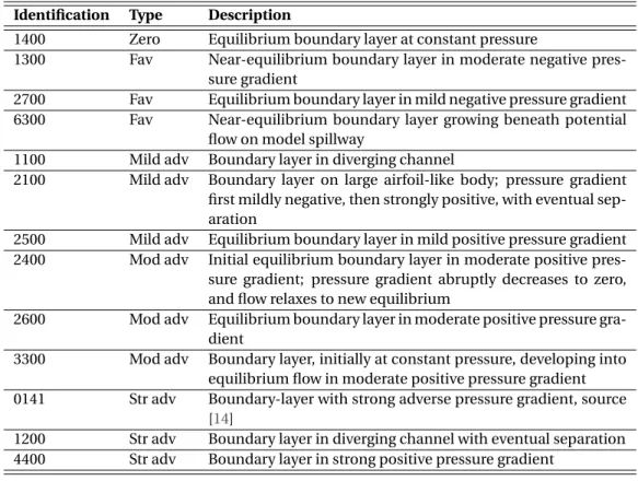
EDDYBL comes with configuration files which mimic the experiments described in the 1968 AFOSR-IFP-Stanford conference proceedings [4]. From this data source, we se-lected one zero pressure-gradient flow, and 12 flows from other types of available pres-sure gradients, which range from favourable (d ¯p/d x < 0) to strongly adverse (d ¯p/d x > 0) gradients. These 13 flows are described in table2.1. The identification number of each flow is copied from Ref.4. According to Ref.37, the flows are identified as being ’mildly adverse’, ’moderately adverse’ etc, based upon qualitative observations of the velocity profile shape with respect to the zero-pressure gradient case. We plotted the experimen-tally determined, non-dimensional, streamwise velocity profiles in Figure2.1. As usual, the normalized streamwise velocity is defined as u+≡ ¯u1/pτw/ρ, where τwis the wall-shear stress. The normalized distance to the wall, displayed on the horizontal axis of Figure2.1, is y+≡ x2pτ
w/ρ/ν. Too much weight should not be given to the classifica-tions of the severity of the adverse gradients, since some flows (such as 2400) experience multiple gradient types along the spanwise direction. Also, when we try to justify the classification based upon the velocity profile shape we find some discrepancies. For in-stance, based upon the profile shape alone, we would not classify flow 1100 as mildly adverse, or 2400 as moderately adverse.
To obtain an estimate of the spread in closure coefficients, we calibrate the k − ε model for each flow of table2.1separately, using one velocity profile as experimental data.
Use of experimental data in the viscous wall region is worthy of a separate discus-sion. On one hand, Reynolds stresses tend to zero when approaching the wall, so that calibrating the turbulence model using data from the first few wall units does not really make sense; moreover, in the whole viscous layer the model is dominated by damp-ing functions (2.3), not calibrated here, introduced to enforce asymptotic consistency as
y+→ 0. As a consequence, little information is obtained from the measurements here. On the other hand, obtaining reliable measurements close to the wall can be difficult due to limited spatial resolution, see e.g. [10]. Therefore, most experimental datasets of [4] do not include points in this region. Additional difficulties may arise according to the experimental technique in use: for instance, outliers due to additional heat losses near the wall are not uncommon in hot-wire measurements, and special corrections are needed to fix the problem [15]. Numerical results from Direct Numerical Simulations (DNS) could be used instead of experimental data sets. Nevertheless, there is little DNS data with high enough values of the friction Reynolds number Reτto allow for a suffi-ciently extended logarithmic region (see [24] for a recent survey).
More generally, our goal is to introduce and test a methodology that can be applied to complex, high-Re flows for which DNS is simply not feasible. The effect of excluding near-wall data from the calibration data set is investigated through numerical experi-ments presented in Section2.5.2.
2.4.
M
ETHODOLOGY
: C
ALIBRATION AND
P
REDICTION
Our methodology consists of two major parts: calibration and prediction. In the cali-bration stage (Section2.4.1) posterior distributions on closure coefficients are identified
2
Table 2.1: Flow descriptions, source [4].
Identification Type Description
1400 Zero Equilibrium boundary layer at constant pressure
1300 Fav Near-equilibrium boundary layer in moderate negative
pres-sure gradient
2700 Fav Equilibrium boundary layer in mild negative pressure gradient
6300 Fav Near-equilibrium boundary layer growing beneath potential
flow on model spillway
1100 Mild adv Boundary layer in diverging channel
2100 Mild adv Boundary layer on large airfoil-like body; pressure gradient
first mildly negative, then strongly positive, with eventual sep-aration
2500 Mild adv Equilibrium boundary layer in mild positive pressure gradient
2400 Mod adv Initial equilibrium boundary layer in moderate positive
pres-sure gradient; prespres-sure gradient abruptly decreases to zero, and flow relaxes to new equilibrium
2600 Mod adv Equilibrium boundary layer in moderate positive pressure
gra-dient
3300 Mod adv Boundary layer, initially at constant pressure, developing into
equilibrium flow in moderate positive pressure gradient
0141 Str adv Boundary-layer with strong adverse pressure gradient, source
[14]
1200 Str adv Boundary layer in diverging channel with eventual separation
4400 Str adv Boundary layer in strong positive pressure gradient
101 102 103 104 experimental y+ 10 15 20 25 30 35 40 expe ri m ent al u + 1400, zero 1300, fav 2700, fav 6300, fav 1100, mild adv 2100, mild adv 2500, mild adv 2400, mod adv 2600, mod adv 3300, mod adv 0141, str adv 1200, str adv 4400, str adv
2
for each of a set of 13 boundary-layer flows. These posteriors are then summarized with Highest Posterior Density (HPD) intervals in Section2.4.3. The results will give a first in-dication of the extent to which posterior distributions of turbulence closure coefficients
θ are case-dependent. This stage can also be seen as a setup stage for the predictive
mechanism of our methodology. To make predictions of a new, unseen flow, we com-bine the 13 posterior distributions for θ using p-boxes (Section2.4.4). These p-boxes encapsulate the effect of both the 13 individual posterior uncertainties (due to the data not exactly identifying a single optimal θ, but rather a probability distribution different from a Dirac function), and the variability of θ between cases.
2.4.1.
C
ALIBRATION FRAMEWORKBayesian calibration requires selection of joint prior distribution for the calibration pa-rameters and a joint pdf (or statistical model) describing the likelihood function.
In our turbulence model calibration we have a large number of accurate observa-tions, and a belief that model inadequacy will dominate the error between reality and prediction. In this situation we expect the prior on closure coefficients to be substan-tially less influential than the joint pdf. We therefore impose uniform priors on closure coefficients, on intervals chosen to: (i) respect mild physical constraints, and (ii) ensure the solver converges in most cases.
After the calibration we verify that the posterior pdf is not unduly constrained by the prior intervals: if we find that one of the informed marginal posteriors is truncated, we simply re-perform the calibration with a wider prior range for the truncated coefficient. We also perform a posterior model checking, in the sense that we verify that sufficient overlapping between the posterior model distribution and the calibration data interval exists.
To specify the joint likelihood we start from the framework of Cheung et. al. [3], who use a multiplicative model inadequacy term, modelled as a Gaussian process in the wall-normal direction. Multiplicative error models are less common than additive errors (like Equation (1.6) in Section1.3), but may be useful in many engineering situations: here, it allows to enforce automatically that the random velocity profiles satisfy a no-slip wall condition (see [3]). By considering multiple different flows we have additional modelling choices. Unlike Cheung et. al., we choose to calibrate closure coefficients and model-inadequacy hyper-parameters independently for each flow, and examine the variability between flows in a post-calibration step.
Let the experimental observations from flow-case k ∈ {1,··· , NC} be zk= [z1k,··· , zNkk]. Here Nkis the number of scalar observations in flow-case k, and zikis the scalar observa-tion at locaobserva-tion y+,i
k > 0, where in the following we work in y+-units. Following Ref.3, we assume the observation noise λk= [λ1k,··· ,λNkk] is known and uncorrelated at all mea-surement points. Furthermore, the closure coefficients and flow parameters for case k are denoted θk and tk respectively. The flow parameters include specification of the pressure-gradient as a function of the x-coordinate. The observation locations y+
k, noise
λk, and flow parameters tk are modelled as precisely known explanatory variables. In the case that substantial uncertainties existed in the experiments these could be mod-elled stochastically as nuisance parameters.
2
A statistical model accounting for additive Gaussian noise in the observations via an additive term and model inadequacy via a multiplicative term is: ∀k ∈ {1,··· , NC}
zk= ζk(y+k) + ek, (2.15a)
ζk(y+k) = ηk(y+k) · u+(y+k,tk;θk), (2.15b) where u+(·,·;·) is the simulation code output, and the multiplication is applied element-wise to its arguments. Observational noise is modelled as
ek∼ N(0,Λk), Λk:= diag(λk),
and the model-inadequacy term ηk(·) is a stochastic process in the wall-distance y+ modelling the relative error between the code output and the true process. Therefore (2.15a) represents the difference between the true process ζkand the measurement ob-servations, and (2.15b) the difference between ζkand model predictions. Together they relate θkto zk.
Cheung et. al. consider three models of this form, which differ only in the modelling of η. They compared the posterior evidence, and showed that modelling η as a correlated Gaussian process yielded by far highest evidence of the three models considered [3]. We therefore adopt the same strategy and model each ηk as a Gaussian process with unit mean (dropping the subscript k for convenience):
η ∼ GP(1,cη), (2.16) and the simple, homogeneous covariance function
cη(y+, y+′| γ) := σ2exp " −µ y +− y+′ 10αl ¶2# , (2.17)
where y+ and y+′represent two different measurement points along the velocity pro-file, and l is a user-specified length scale. We fix this length scale to 5.0, which is the y+ value that denotes the end of the viscous wall region. The smoothness of the model-inadequacy term is controlled by the correlation-length parameter α, and its magnitude by σ. Both α and σ are unknown, and must be obtained via calibration from the data, and form a hyper-parameter vector γ := [α,σ].
A more boundary-layer specific model than (2.16), is described in Ref.23. It attempts to account for the multi-scale structure of the boundary layer by allowing the correlation length to vary in y+direction. Together (2.15b) and (2.16) imply the relative model inad-equacy σ is independent of y+, and that the correlation length is the same throughout the boundary layer. This model may be generalized to multiple dimensions by replacing
η(·) with a multi-dimensional Gaussian process. See [12] for a thorough discussion of the role of the covariance term.
A consequence of the above modelling choices is that the true process ζ is also mod-elled as a Gaussian process:
ζ | θ,γ ∼ GP(µζ,cζ) (2.18)
µζ(y+| θ) = u+(y+,t;θ)
cζ(y+, y+′| θ,γ) = u+(y+,t;θ) · cη(y+, y+′| γ)·
2
which is still centered around the code output. The assumption of normality is made mainly for convenience, and more general forms are possible. See Section2.4.5for a discussion on the choice of statistical model.
The likelihood evaluated at the measurement locations y+,i can now be written for each flow case k independently as:
p(z | θ,γ) =p 1 (2π)N|K |exp · −1 2d T K−1d ¸ , d := z − u+(y+) K := Λ + Kζ. (2.19) where £ Kζ ¤ i j:= cζ(y+,i, y+,j|θ,γ).
Since in general the computational grid does not coincide with measurement locations we linearly interpolate the code output at y+,iwhere needed.
Note that the statistical model is based only on velocity data, and does not include constraints on other physical quantities, like e.g. the Reynolds stresses or the turbulent kinetic energy k. This choice is consistent with the fact that our version of k−ε is not real-izable, and as such it does not contain any modelling assumption to prevent the normal Reynolds stresses from becoming negative, but only enforces them to satisfy physical constraints through the application of limiters. If we were to calibrate realizable k −ε we would try to preserve the realizability conditions. This would require adding constraints to the likelihood function so that zero probability is assigned to parameter combinations leading to unrealizable turbulence states.
2.4.2.
P
RIORS FORθ
ANDγ
Unlike Cheung et. al., we do not treat all closure coefficients as independent random variables in the prior. Instead we use the physical relations described in Section2.2.1to constrain the value of two closure coefficients. Specifically we fix Cǫ1, by rewriting (2.13) as
Cǫ1= Cǫ2 P/ε+
P/ε − 1
P/ε , (2.20)
where, similar to Ref.25, we fix the ratio P /ε to 2.09. In our results, this choice locates the mode of the posterior for Cε2relatively close to the standard value of 1.92. If we in-stead would have used a different (experimentally determined) value of P /ε, the mode
Cε2would be located elsewhere. Whether or not our choice is reasonable has to be de-termined by the ability of the posterior distributions to capture the observed data, as outlined in Section2.5.3. Two other possibilities we do not employ are: (i) to move P /ε into θ and calibrate it along with the other parameters with some suitable prior, or (ii) model P /ε as an aleatory uncertainty, using the P /ε data from Ref.36to construct an
2
approximate pdf p(P /ε). Also, we fix σεusing (2.12). Such a choice avoids running the boundary-layer code with non-physical parameter combinations.
All priors, for both the closure coefficients θ and hyper-parameters γ, are indepen-dent uniform distributions. The choice of interval end-points was made based on three factors: the spread of coefficients recommended in the literature, the range of coeffi-cients for which the solver was stable, and avoidance of apparent truncation of the pos-terior at the edge of the prior domain. The range we used is specified in Table2.2. We Table 2.2: The empirically determined range (absolute and relative to nominal value) of the uniform prior distributions.
coefficient left boundary right boundary
Cǫ2 1.15 (-40%) 2.88 (+50%) Cµ 0.054 (- 40 %) 0.135 (+50 %) σk 0.450 (-45 %) 1.15 (+50 %) κ 0.287 (-30 %) 0.615 (+50 %) σ 0.0 0.1 logα 0.0 4.0
chose uniform distributions because we lack confidence in more informative priors for these parameters. We note however that some reasonable, informative priors can be ob-tained using the classical framework for coefficient identification (c.f. Section2.2.1) in combination with multiple experimental measurements from different sources [25].
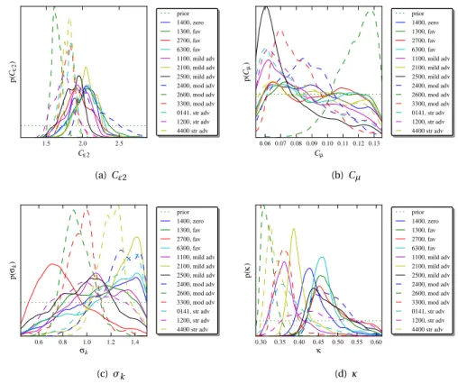
To obtain samples from the posterior distributions p (θ | z), we employed the Markov-chain Monte Carlo (McMC) method [9]. We subsequently approximated the marginal pdf of each closure coefficient using kernel-density estimation, using the last 5,000 (out of a total of 40,000) samples from the Markov chain. It was observed that at 35,000 sam-ples, the Markov chain was in a state of statistical convergence.
2.4.3.
S
UMMARIZING POSTERIORS: HPD
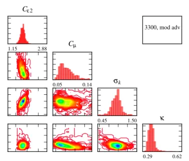
INTERVALSThe methodology of Section2.4.1will be applied to 13 flow cases, resulting in 13 poste-riors on [θ,γ]. The large amount of information (see e.g. Figure2.2and2.3in the results section) is difficult to visualize. In other words the posteriors must be summarized, and we do this with intervals. In the remainder we make the assumption that closure coef-ficients are approximately independent and uncorrelated. This is justified by Figure2.3. This assumption allows us to work with 1d marginal pdfs of the coefficients, rather than the full multi-dimensional posteriors.
We compute Highest Posterior Density (HPD) intervals on 1d marginals to summa-rize the posteriors. An HPD interval is a Bayesian credible interval which satisfies two main properties, namely:
1. The density for every point inside the interval is greater than that for every point outside the interval.
2
We use the algorithm of Chen et. al. [2] to approximate the HPD intervals using the ob-tained McMC samples. To do so, we first sort the samples of the Q closure coefficients
θq, q = 1,2,··· ,Q in ascending order. Then, if we let {θqj, j = 1,2,··· , J} be the McMC sam-ples from p¡θq| z¢, the algorithm basically consists of computing all the 1 − β credible
intervals and selecting the one with the smallest width. For a given j , we can use the em-pirical cumulative-distribution function to approximate the 1 −β interval by computing the first θqs which satisfies the inequality
J X i =j ✶θq i≤θ q s ≥ £ J¡1−β¢¤, (2.21) where ✶θq i≤θ q
s is the indicator function for θ
q i ≤ θ
q s and
£
J¡1−β¢¤ is the integer part
of J¡1−β¢. Secondly, if we let θ(i )q be the smallest of a set {θqi}, then the first θqs for which (2.21) is satisfied simply is θ([qJ(1−β)]). Thus, the jthcredible interval is given by
θ(q
j +[J(1−β)]) −θ q
(j)and the HPD interval for θ
qis found by solving min j θ q (j +[J(1−β)]) −θ q (j), 1 ≤ j ≤ J − £ J¡1−β¢¤. (2.22)
The algorithm of Chen assumes a uni-modal posterior pdf, although it could possibly be extended to deal with multi-modal pdfs [2]. This assumption is shown to be justified in our case in Section2.5.5.
2.4.4.
P
REDICTIVE FRAMEWORK: P-
BOXESSo far we have only discussed identification of θ for flows with data. The final purpose of this work is to establish uncertainties on k − ε model predictions under flow conditions
t∗at which no measurements are available. To achieve this we must assess the effect of all sources of uncertainty on the model prediction at t∗. We require a method that can simultaneously represent solution variability within- and between the posteriors p(θ,γ |
zk,tk), k = 1,2,··· , NC, where NC= 13 in this work.
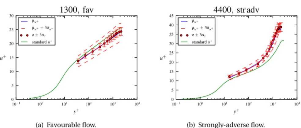
Our approach is to construct a probability box (p-box) for the output of the model at the new condition t∗, using coefficients sampled from the HPD intervals of each of the 13 cases. A p-box is commonly used to visualize possible outcomes due to a combination of epistemic and aleatory uncertainty [22]. Examples of p-boxes are shown in Figure2.13. In our case - roughly speaking - the slant of the box represents the width of individual HPD intervals, and the width of the box the variability between HPD intervals obtained from calibrations against different data sets. More precisely they can be interpreted as bounds on the ζ (or u+) value at any particular probability level, and therefore can be used to construct confidence intervals on the true process ζ or code output u+.
We define our p-box as follows: For flow case k, let Θ50
k be a uniformly distributed random variable on the box given by the 50% HPD intervals of the posterior for θ. Prop-agate this variable through the flow-code for u+to obtain
2
a random variable representing the effect of posterior uncertainty in case k on the model output at conditions t∗. Here y+
∗is the location at which an uncertainty estimate is re-quired, which need not correspond to a sample location in any of the calibrated flow cases. Let Fk(u+) = P(Zk≤ u+) be the cumulative density function of Zk. Then the p-box D is defined by D(u+) := {r ∈ [0,1] | F (u+) ≤ r ≤ F (u+)}, F (u+) := min k∈{1,...,13}Fk(u +), (2.23) F (u+) := max k∈{1,...,13}Fk(u +)
i.e. the envelope formed by this collection of k cdfs. To construct a worst-case 90% con-fidence interval we find the end-points u+and u+such that
F(u+) = 0.05,
F (u+) = 0.95.
The interval I = [u+,u+] is our final estimate of solution uncertainty due to modelling inadequacy in the k − ε model for u+(y+
∗) at conditions t∗.
To construct the p-box in (2.23) numerically we use empirical cdfs:
Fk(u+) = P ¡ Zk≤ u+ ¢ ≈1 S S X j =1 ✶u+ j≤u+, (2.24) where u+
j are S samples from Zkobtained using Monte-Carlo. An approximation to D is then readily calculated.
Note that because Zkis based only on the flow-code output and not on the true pro-cess ζ, the effect of the model inadequacy term η is not included in our estimates. If a variable other than u+were of interest, we could define the p-box in exactly the same way (using skin-friction Cf as an example):
Yk(x) := Cf(x, t∗;Θ50k ).
That this is possible is a consequence of representing model inadequacy via closure co-efficients. It is not possible if we base estimates on η-like terms. For the validity of the confidence intervals we are relying on the uncertainties in θ accounting for the majority of model error. We acknowledge that the choice of 50% HPD intervals plays a role in the p-box size, and this tuning parameter could be eliminated by replacing Θ50k and Γ50k by the posteriors for case k, at the cost of increasing the size of the p-boxes.
2.4.5.
D
ISCUSSIONIn the above we are attempting to capture model error in two different ways:
1. Via the traditional (Kennedy and O’Hagan) Gaussian process (GP) “model discrep-ancy” term, η(·), and
![Table 3.1: Traditional closure coefficient values [ 24 ].](https://thumb-eu.123doks.com/thumbv2/123doknet/2617043.58227/54.735.154.650.118.450/table-traditional-closure-coefficient-values.webp)
![Figure 3.3: Experimental |β T | values for all flows but 1400 and 0141. Source [ 4 ]. Table 3.2: Flow descriptions, source [ 4 ].](https://thumb-eu.123doks.com/thumbv2/123doknet/2617043.58227/56.735.207.580.101.359/figure-experimental-values-flows-source-table-descriptions-source.webp)