Reduction of acoustic fields of horn-like structures by optimization of network resonators

(1)

HAL Id: tel-01386782

https://pastel.archives-ouvertes.fr/tel-01386782

Submitted on 24 Oct 2016

HAL is a multi-disciplinary open access archive for the deposit and dissemination of sci-entific research documents, whether they are pub-lished or not. The documents may come from teaching and research institutions in France or abroad, or from public or private research centers.

L’archive ouverte pluridisciplinaire HAL, est destinée au dépôt et à la diffusion de documents scientifiques de niveau recherche, publiés ou non, émanant des établissements d’enseignement et de recherche français ou étrangers, des laboratoires publics ou privés.

optimization of network resonators

Bin Wang

To cite this version:

Bin Wang. Reduction of acoustic fields of horn-like structures by optimization of network resonators. Materials. Université Paris-Est, 2015. English. �NNT : 2015PESC1155�. �tel-01386782�

(2)

École doctorale Sciences, Ingénierie et Environnement THÈSE de doctorat Discipline : Mécanique Présentée par: Bin WANG Sujet de la thèse :

REDUCTION OF ACOUSTIC FIELDS OF

HORN-LIKE STRUCTURES BY OPTIMIZATION OF

NETWORK RESONATORS

Soutenue publiquement le DD MM YY devant un jury composé de :

M. Mabrouk BEN TAHAR Université de Technologie de Compiègne Examinateur

M. Michel BERENGIER IFSTTAR Rapporteur

M. Denis DUHAMEL Ecole des Ponts ParisTech Directeur de thèse

M. Philippe KLEIN IFSTTAR Examinateur

(3)

(4)

Résumé

Le bruit généré dans la zone de contact entre un pneumatique et une route peut être amplifié par des dièdres constitués des surfaces du pneumatique et la route. Cette étude est consacrée à l’optimisation et à la conception de bandes de roulement et de textures de la route pour réduire l’amplification de l’effet dièdre sur la base de l’annulation de sons. Les bandes de roulement et les textures de la route peuvent être considérées comme deux réseaux dans la zone de contact. Les surfaces du pneu-matique et de la route peuvent être considérées comme des baffles. Un modèle de réseau à baffle est constitué pour le système pneumatique / chaussée, et des procédés de couplage multi-domaines sont développés pour le calcul des champs acoustiques autour des réseaux à baffles. Avec ce modèle, la réduction des amplifications de l’effet dièdre par les réseaux peut être estimée. Étant donné que les réductions sont autour des fréquences de résonance de l’air à l’intérieur des réseaux, des méthodes numériques simples pour estimer les fréquences de résonance sont développées. Afin de concevoir des réseaux pour obtenir les fréquences de résonance recherchées, une méthode d’optimisation sur la base des algorithmes génétiques est proposée. Les méthodes d’estimation des fréquences de résonance sont validées avec des mesures. Les méthodes d’optimisation et le modèle des réseaux bafflés sont également vérifiées par les expériences. Une structure avec un cylindre en bois et une feuille de contre-plaqué est construite pour les validations. Un vrai pneumatique sur une feuille de contreplaqué est également mesuré et calculé avec les méthodes proposées. Les ban-des de roulement sont optimisées avec les méthoban-des proposées. Plusieurs réductions des amplifications de l’effet dièdre peuvent être vues et sont estimées avec les méth-odes de couplage multi-domaines. La dimension des motifs de texture de la route est également étudiée afin de trouver les réductions maximales des amplifications. Mots clés : Bruit; Pneumatique; Route; Effet dièdre; Résonance; Correction de longueur; Résonateur acoustique; Sculpture; Texture; Optimisation.

(5)

(6)

Abstract

The noise generated in the contact zone between a tire and a road can be amplified by horns constituted of the surfaces of the tire and the road. This study is devoted to the optimization and the design of tire treads and road textures for reducing the amplification of horn effect based on the sound cancellation. The tire treads and the road textures can be considered as two dimensional networks in the contact zone. The surfaces of the tire and the road can be seen as flanges. A model of flanged networks is established for the tire/road system, and multi-domain coupling methods are de-veloped for the calculation of the acoustic fields around the flanged networks. With this model the reductions of the amplifications of horn effect by the networks can be estimated. Since the reductions are around the resonant frequencies of air inside the networks, simple numerical methods for estimating the resonant frequencies are developed. In order to design the networks to get wanted resonant frequencies, an optimization method based on genetic algorithms is proposed. The methods for esti-mating the resonant frequencies are validated with measurements. The optimization methods and the model of the flanged networks are also proved to be effective by the experiments. The wooden networks between a wooden cylinder and a sheet of ply-wood are built for the validation. A real tire on a sheet of plyply-wood is also measured and calculated with the proposed methods. Last the tire treads are optimized with the optimization methods. Multiple reductions of the amplifications of horn effect can be seen and are estimated with the multi-domain coupling methods. The road brick dimension is also investigated in order to find the maximum reductions of the amplifications.

Keywords: Noise; Tire; Road; Horn effect; Pipe resonance; End correction; Acoustic network resonator; Tire treads; Road textures; Optimization.

(7)

(8)

Long Résumé

Le bruit généré par le trafic automobile est responsable d’une grande partie de la pollution de l’environnement sonore. Grace à la technologie moderne, le bruit des moteurs de voiture et d’autres pièces mécaniques a été considérablement réduit. Par conséquent, le bruit des pneumatiques en interaction avec la route est de plus en plus perceptible. Au-dessus d’une vitesse de 50km/h, le bruit généré par les pneuma-tiques roulant sur la route est le bruit dominant [1]. Le bruit des pneumatiques de poids-lourds domine également lorsque la vitesse est supérieure à 80km/h. Ainsi une réduction de la génération du bruit de contact pneumatique / chaussée va grandement améliorer l’environnement en bordure de route et la qualité de vie associée.

Il est essentiel de comprendre les mécanismes de génération du bruit de contact pneumatique / chaussée pour faciliter la recherche de sa réduction sans compromettre la sécurité routière. Ainsi, les mécanismes de la génération et du rayonnement du bruit de roulement provoqué par l’interaction entre un pneumatique et la surface d’une route ont reçu une attention considérable au cours des dernières décennies. Les phénomènes physiques responsables de la génération et du rayonnement du bruit de contact pneumatique / chaussée sont bien connus, et sont essentiellement les vibrations de pneumatiques, le pompage d’air, l’effet dièdre et les résonances d’air.

L’objectif de cette étude est concentré sur la réduction de l’effet dièdre par la résonance de l’air à l’intérieur des conduits entre le pneumatique et la route. Le bruit généré dans la zone de contact peut être amplifié par les dièdres comprenant des surfaces du pneumatique et de la route. Les recherches antérieures sur l’effet dièdre ont seulement considéré un pneumatique et une route lisses. Dans ce travail, nous prenons en compte les bandes de roulement et les textures de la route dans cet effet dièdre. Le couplage entre les résonances de l’air et l’effet dièdre sera étudié dans le même modèle.

Un modèle de réseau bafflé est établi pour calculer les champs acoustiques dans le système pneumatique / chaussée. Les bandes de roulement et la texture de la route peuvent être considérées comme deux réseaux tridimensionnels dans la zone

(9)

de contact entre le pneumatique et la route. Les surfaces du pneumatique et de la route peuvent être considérées comme des baffles. Dans ce modèle à la fois l’effet dièdre et la résonance de l’air sont pris en compte. Il peut être utilisé pour estimer la réduction de l’effet dièdre en utilisant les résonateurs du réseau. L’impédance de rayonnement peut être pris en compte à l’extrémité d’un tuyau. En calculant un simple tuyau droit à bride avec les méthodes d’impédance de rayonnement, la description physique de la propagation des ondes et l’interaction entre les champs acoustiques en dehors de la structure et à l’intérieur du tuyau sont présentés clairement. Pour des baffles et des réseaux complexes les méthodes de couplage multi-domaines sont proposées pour obtenir les solutions. Dans les procédés de couplage multi-domaine, le domaine acoustique est divisé en sous-domaines extérieur et intérieur, sous-domaines qui sont couplés aux interfaces entre eux par la continuité de la pression et de la vitesse. Nous utilisons des méthodes d’éléments de frontières pour obtenir un système d’équations pour le sous-domaine extérieur. Si le sous-domaine intérieur est un tuyau droit, nous pouvons utiliser la matrice de transfert pour le résoudre. La théorie de Miles [2] est adaptée pour calculer deux jonctions de réseau tridimensionnel, on peut donc combiner la matrice de transfert et la théorie de Miles pour résoudre un réseau complexe. Les méthodes numériques (telles que les méthodes d’éléments de frontière et les méthodes d’éléments finis) peuvent être utilisées pour des réseaux tridimensionnels. Bien entendu, les méthodes numériques peuvent également être appliquées à des cas à une ou deux dimensions. En résolvant le problème couplé, la pression et la vitesse sur l’ensemble de la frontière peuvent être obtenues. Puis, les champs acoustiques peuvent être calculés par une formule intégrale. Les formes de tuyau en T sont résolus par la méthode des éléments de frontière et les méthodes de couplage multi-domaines. De bons accords entre ces méthodes prouvent la fiabilité des méthodes de couplage multi-domaines. Comme pour les deux réseaux tridimensionnels, les procédés de couplage multi-domaine permettent de ne pas mailler le réseau, ils sont plus efficaces que les méthodes d’éléments de frontière. Les pertes dues aux conductivités visqueuses et thermiques à la paroi du tube peuvent être prises en compte dans les méthodes de couplage multi-domaines afin d’améliorer la précision des solutions. Un tuyau droit à bride et un réseau bridé sont calculés pour comparer les méthodes de couplage multi-domaine avec et sans pertes.

D’importantes réductions des amplifications de l’effet dièdre peuvent être vues autour des fréquences de résonance. Par conséquent des méthodes numériques sim-ples (méthode des éléments finis) pour estimer les fréquences de résonance de l’air à l’intérieur des réseaux sont développées. Il n’est pas nécessaire de calculer les champs acoustiques à l’extérieur des baffles pour obtenir les fréquences de résonance, ce qui

(10)

VII est consommateur de temps de calcul. Nous pouvons obtenir les fréquences de ré-sonance facilement en résolvant un problème de valeurs propres par la méthode des éléments finis. Nous avons développé un programme à cet effet dans lequel nous de-vons saisir les paramètres tels que la dimension de réseau, les conditions aux limites et ou les corrections de longueur. Puisque les réseaux bridés non seulement ont des extrémités fermées, mais aussi des extrémités ouvertes, les corrections d’extrémité aux extrémités ouvertes doivent être calculées en premier. Ces corrections seront utilisées dans l’estimation des fréquences de résonance. Basé sur les méthodes numériques (méthodes d’éléments de frontière) proposées dans [3], les corrections des extrémités ouvertes bafflées peuvent être obtenues. Les fréquences de résonance de plusieurs réseaux à brides sont estimées par nos méthodes proposées et comparées avec les ré-sultats de champs acoustiques à partir desquels nous pouvons aussi voir les fréquences de résonance. De bons accords peuvent être observés.

Pour un réseau spécifié, nos méthodes peuvent donner les fréquences de ance. Toutefois, si nous concevons le réseau pour obtenir les fréquences de réson-ance recherchées, une méthode d’optimisation des structures de réseau est néces-saire. Les fréquences de résonance dépendent de la structure du réseau. Un procédé d’optimisation sur la base des algorithmes génétiques et des méthodes d’estimation pour des fréquences de résonance est développé à cet effet. Les paramètres de la di-mension de réseau tels que les types de jonction, les positions de jonction et la surface de section transversale peuvent être optimisés. Nous choisissons trois types de jonc-tions pour construire le réseau: un T tourné vers la gauche, un T tourné vers la droite et une jonction en croix. Deux fonctions objectifs sont définies. L’une est pour une seule fréquence de résonance déterminée, et l’autre est pour un nombre maximal de fréquences de résonance dans une plage de fréquences spécifiée. Avec cette méthode, les deux réseaux tridimensionnels avec la fréquence cible ou le nombre maximal de fréquences de résonance dans une bande de fréquences peuvent être trouvés. Nous pouvons réduire les amplifications de l’effet dièdre autour de ces fréquences de réso-nance optimisées. Plusieurs exemples d’optimisation de deux réseaux avec et sans baffles sont donnés.

Le modèle proposé, les méthodes de calcul, les méthodes d’estimation pour les fréquences de résonance et les méthodes d’optimisation sont validés avec des mesures de plusieurs tuyaux bafflés en bois et un vrai pneumatique. D’abord un guide d’onde droit en bois et un réseau en bois entre un cylindre de bois et une feuille de con-treplaqué sont respectivement mesurés. Les tendances concernant la pression sonore sont similaires aux résultats prédits par les méthodes de couplage multi-domaine, et de bons accords entre les résultats mesurés et prévus peuvent être vus. Les fréquences

(11)

de résonance sont très proches des estimations. Ensuite, le réseau est optimisé afin d’obtenir un nombre maximum de fréquences de résonance inférieures à 2000Hz. Qua-tre fréquences de résonance peuvent êQua-tre trouvées. Nous avons calculé et mesuré les champs acoustiques pour l’un des réseaux optimisés. D’après les résultats prévus, nous pouvons voir les fréquences de résonance optimisées. Les résultats prédits concordent bien avec les résultats mesurés. Ensuite un réseau non bafflé est optimisé pour une des fréquences de résonance spécifiées. A partir des champs acoustiques mesurés, nous pouvons voir la fréquence de résonance ciblée qui est très proche de la fréquence de résonance prédite. Finalement un véritable pneumatique sur une surface plane est mesuré et calculé. En raison de l’erreur sur la longueur estimée de la zone de contact, les résultats prévus sont en accord partiel avec les résultats mesurés. Dans notre ex-périence, la zone de contact ne peut pas être pressée fermement sur le sol car la charge que l’on utilise est très inférieure à la charge d’un véhicule réel. Ainsi, la longueur de la zone de contact n’est pas vraiment estimée correctement.

Pour l’optimisation des bandes de roulement et de la texture de la route, nous supposons que le pneumatique peut être appuyé fermement sur la route dans la zone de contact. Les bandes de roulement sont optimisées de deux manières. Dans la première optimisation, on insère le réseau optimisé un par un pour les pics de fréquence ciblés. Dans la seconde optimisation, les réseaux optimisés ont un nombre maximum de fréquences de résonance inférieures à 2000Hz. Pour les deux types de réseaux optimisés, de multiples réductions des amplifications de l’effet dièdre peuvent être vues à travers les calculs avec les méthodes de couplage multi-domaines. La dimension de la texture de route est étudiée afin de trouver les réductions maximales des amplifications de l’effet dièdre jusqu’à 2000Hz. Le nombre maximum de fréquences de résonance que nous pouvons trouver est 3. Nous pouvons voir trois réductions claires des champs acoustiques calculés par les méthodes de couplage multi-domaines.

(12)

Long Summary

Noise generated by traffic is responsible for a great portion of environmental noise pollution. Thanks to modern technology, noise from car engines and other mechanical parts has been significantly reduced. Therefore, noise from tire and road interaction is becoming increasingly noticeable. Above the moderate speed of 50km/h, the sound generated by the tires rolling over the road is the dominant noise [1]. Tire noise from trucks also dominates when the speed is higher than 80km/h. Hence a reduction in tire/road noise generation will greatly improve the roadside environment and the associated quality of life.

It is essential to understand the mechanisms of noise generation to facilitate the search for quiet tire/road surface without compromising road safety. So the mecha-nisms of the generation and radiation of rolling noise caused by the interaction between a tire and the surface of a road have received considerable attention over the past few decades. The physical phenomena responsible for the generation and radiation of tire/road contact noise are well known, basically due to tire vibrations, air-pumping, horn effect and air resonances.

The focus of this study is put on the reduction of horn effect by the resonance of air inside the pipes between the tire and the road based on the sound cancellation. The noise generated in the contact zone can be amplified by the horns comprised of the surfaces of the tire and the road. Previous researches on the horn effect only investigate smooth tires and roads. In this work we take into account the tire treads and the road textures in the calculation of horn effect. The air resonances and horn effect will be studied in the same model.

A model of flanged networks is established for calculating the acoustic fields around the tire/road system. The tire treads and the road textures can be considered as two dimensional networks in the contact zone between the tire and the road. The surfaces of the tire and the road can be seen as flanges. In this model both the horn effect and the air resonance are taken into account. It can be used to estimate the reduction of the horn effect by using the network resonators. Radiation impedance can be

(13)

applied to the calculation of the simple flange and pipe. By computing a simple flanged straight pipe with the radiation impedance methods, the physical description of the wave propagation and the interaction between the acoustic fields outside the flange and inside the pipe are presented clearly. For the complex flanges and networks multi-domain coupling methods are proposed to get the solutions. In the multi-domain coupling methods, the acoustic domain is divided into an exterior subdomain and an interior subdomain which are coupled at the interfaces between them by the continuity of pressure and velocity. We use boundary element methods to get an equation system for the exterior subdomain. If the interior subdomain is one dimensional straight pipe, we can use transfer matrix to solve it. The theory of Miles [2] is suitable for calculating two dimensional network junctions, so we can combine the transfer matrix and the theory of Miles to solve a complex network. Numerical methods (such as boundary element methods and finite element methods) can be used for three dimensional networks. Of course the numerical methods can also be applied to the one and two dimensional cases. By solving the coupled problem, the pressure and velocity on the whole flange can be obtained. Then the acoustic fields can be calculated by an integral formula. A flanged T shaped pipe is solved by the boundary element method and multi-domain coupling methods. Good agreements between these methods prove the reliability of the multi-domain coupling methods. Since for two dimensional networks the multi-domain coupling methods don’t use network meshes, they are more effective than boundary element methods. The viscous and thermal conductivity losses at the pipe walls can be taken into account in the multi-domain coupling methods in order to improve the accuracy of the solutions. A flanged straight pipe and a flanged network are calculated to compare the multi-domain coupling methods with and without losses.

Large reductions of the amplifications of horn effect can be seen around the res-onant frequencies. Therefore simple numerical methods (finite element methods) for estimating the resonant frequencies of air inside the flanged networks are developed. It is not necessary to calculate the acoustic fields outside the flanges to get the reso-nant frequencies, which is quite time-consuming. We can get the resoreso-nant frequencies easily by solving an eigenvalue problem with the finite element method. We developed a program for this purpose where we should input the parameters such as the network dimension, boundary conditions and end corrections. Since the flanged networks not only have closed ends but also have open ends, the end corrections of the open ends should be calculated first. These end corrections will be used in the estimation of resonant frequencies. Based on the numerical methods (boundary element methods) proposed in [3], the corrections of the flanged open ends can be obtained. The resonant

(14)

XI frequencies of several flanged networks are estimated by our proposed methods and compared with the results of acoustic fields from which we can also see the resonant frequencies. Good agreements can be seen.

For a specified flanged network, our proposed methods can give the resonant fre-quencies. However, if we design the network to get the wanted resonant frequencies, optimization methods of the network structures are requisite. The resonant frequen-cies depend on the network structures. An optimization method based on genetic algorithms and the estimation methods for the resonant frequencies is developed for this purpose. Parameters of the network dimension such as junction types, junction positions and cross sectional area can be optimized. We choose three types of junc-tions to build the network: left T junction, right T junction and cross junction. Two objective functions are defined. One is for a single specified resonant frequency, and the other one is for the maximum number of resonant frequencies within a specified frequency range. With this method, the two dimensional networks with the targeted or the maximum number of resonant frequencies within a frequency range can be found. We can reduce the amplifications of horn effect around these optimized resonant fre-quencies. Several optimization examples of unflanged and flanged two dimensional networks are given.

The proposed model, computational methods, estimation methods for the resonant frequencies and the optimization methods are validated with measurements of several wooden flanged pipes and a real tire. First a straight wooden pipe and a wooden network between a wooden cylinder and a sheet of plywood are respectively measured. The tendencies of sound pressure are similar to the results predicted by the multi-domain coupling methods, and good agreements between the measured and predicted results can be seen. The resonant frequencies are very close to the estimations. Then the network is optimized in order to get a maximum number of resonant frequencies within 2000Hz. Four resonant frequencies can be found. We calculated and measured the acoustic fields for one of the optimized networks. From the predicted results we can see the optimized resonant frequencies. The predicted results agree well with the measured results. Next an unflanged network is optimized for a specifed resonant frequencies. From the measured acoustic fields we can see the targeted resonant frequency that is very close to the predicted resonant frequency. Last a real tire on a plane surface is measured and calculated. Due to the error of the estimated length of the contact zone, the predicted results partly agree with the measured results. In our experiment, the contact zone may not be pressed firmly in the whole contact zone because the load that we use is much smaller than the load from a real car. So the length of the contact zone may not be estimated correctly.

(15)

For the optimization of the tire treads and the road textures, we assume that the tire can be pressed firmly on the road in the whole contact zone. The tire treads are optimized in two ways. In the first optimization, we insert the optimized networks one by one for the targeted peaks. In the second optimization, the optimized networks have a maximum number of resonant frequencies within 2000Hz. For both types of optimized networks, multiple reductions of the amplifications of horn effect can be seen through the calculations with the multi-domain coupling methods. The road brick dimension is investigated in order to find the maximum reductions of the ampli-fications of horn effect within 2000Hz. Since the maximum number of the resonant frequencies that we can find is 3, we can see three clear reductions from the acoustic fields computed by the multi-domain coupling methods.

(16)

Acknowledgement

I would like to start by thanking my supervisor, Doctor and Professor Denis Duhamel, for his insights, rigorous working attitude and constant guidance on my studies. I am really grateful for the opportunity of studying with him. I would also appreciate Dr. Honoré Yin for his helpful suggestions. Many thanks to Dr. Gwendal Cumunel and Mrs Anne Ferri for their assistances in conducting experiments. Great appreciation is also expressed to my parents for their warm care and support.

Lastly, I would like to take this opportunity to thank my wife, Mayao Cheng, for her great care and love.

(17)

(18)

List of Figures

1.1 Sound generation and enhancement mechanisms of tire/road noise [4] 2

1.2 Horn effect: multiple refections of sound in the horn-like structure . . 4

1.3 (a) Tire on the road; (b) Tire without the road. . . 5

1.4 Pipe resonators in the contact zone between a tire and a road . . . 7

1.5 A sound absorbing wall with quarter-wave resonators. . . 8

1.6 Two axially coupled tubes. . . 9

1.7 T-shaped acoustic resonator. . . 10

1.8 A piston with an infinite baffle. . . 11

1.9 A simple example of a two dimensional wooden network with open and closed ends . . . 14

2.1 (a) Flanged network; (b) Network. . . 19

2.2 (a) Total pressure; (b) Pressure directly from the source and reflected by the flange; (c) Pressure radiating from the network . . . 20

2.3 A straight pipe at the center of a cylinder . . . 21

2.4 Junction . . . 28

2.5 Pressure at the imaginary end of a straight pipe: (a) 200−2000Hz; (b) Around the resonant frequencies . . . 31

2.6 Pressure at receiver R: (a) 200 − 2000Hz; (b) Around the resonant frequencies . . . 32

2.7 T pipe with rectangular flange . . . 33

2.8 Pressure at the imaginary end (z = 0.005m): (a) 200 − 2000Hz; (b) Around the second resonant frequencies . . . 34

2.9 Pressure at point R near flange . . . . 34

2.10 (a) Network between a round surface and a rigid plane surface; (b) The network with open ends. . . 35

(23)

2.12 Half of a tire with a network in the contact zone between a tire and a road . . . 36

2.13 (a) Network 1; (b) Network 2 . . . 37

2.14 Modulus of sound pressure at R: (a) 200 − 200HZ; (b) Around the resonant frequencies . . . 37

2.15 Pressure modulus in a circle around the body (a) Frequency 200Hz; (b) Frequency 1410Hz; (c) Frequency 1455Hz . . . . 38

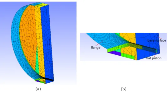
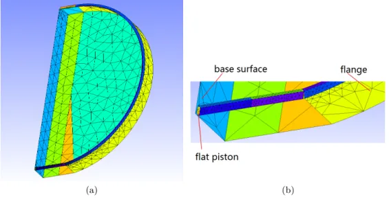
2.16 (a) Meshes of half a cylinder with half of a straight pipe at the center of the contact zone; (b) Details of meshes of the contact zone. . . 39

2.17 Predicted results for a straight pipe between a cylinder and a plane surface . . . 40

2.18 Predicted results for a network between a cylinder and a plane surface: (a) 200 − 2000HZ; (b) Around the resonant frequencies . . . . 40

3.1 Mesh of the boundary element model of a tube with a circular flange (case r/R =1/2) . . . 45

3.2 (a) End corrections divided by pipe radius from [3] (ka<2): (dots) fit formula (3.3) results, (plus sign) BEM results by Dalmont, (straight line) experimental results; (b) Errors between fit formula and BEM results (ka<0.23). (Symbol a in the figures represents the radius r) . . 46

3.3 (a) Half of meshes of the boundary element model of a rectangular tube with a flange of cylinder; (b) Details of the mesh of the tube. . . 47

3.4 End corrections of longitudinal pipes with cylindrical flanges of different widths within 2000Hz (ka < 0.23) . . . . 48

3.5 Standard deviations and mean values of end corrections of longitudinal pipes with cylindrical flanges of different widths . . . 48

3.6 (a) Half of meshes of the boundary element model of a rectangular tube with a part of tire flange; (b) Details of the mesh of the tube. . . 49

3.7 End corrections of a longitudinal pipe with tire flanges of different widths within 2000Hz . . . . 50

3.8 Standard deviations and mean values of end corrections of a longitudi-nal pipe with tire flanges of different widths . . . 50

3.9 T-shaped pipe . . . 52

3.10 Flow chart of Matlab program 2DNRF for calculating network resonant frequencies . . . 55

(24)

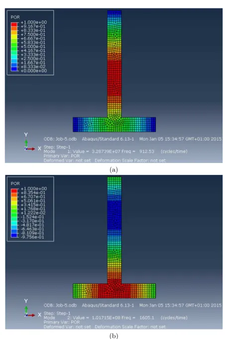
LIST OF FIGURES XXI 3.11 Modes of T pipe within 2000 Hz obtained from Abaqus by 2DNRF: (a)

The first resonant frequency 912Hz; (b) The second resonant frequency 1605Hz. . . . 57

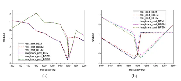
3.12 Total pressure modulus at the open end of branch 3 . . . 58

3.13 Total pressure modulus distributions on the T pipe surface at resonant frequencies within 2000Hz by BEM: (a) The first resonant frequency 914Hz; (b) The second resonant frequency 1610Hz. . . . 58

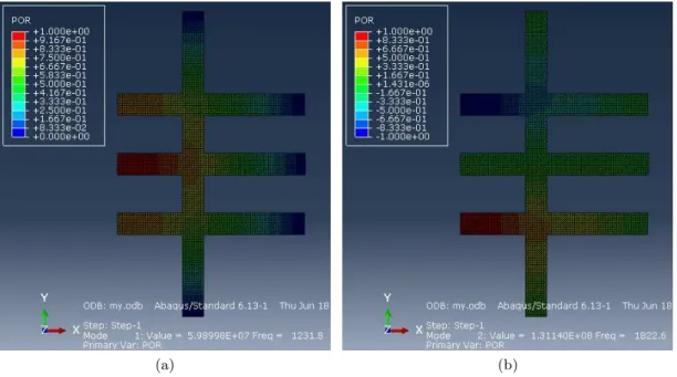
3.14 Modes of half network within 2000 Hz: (a) The first resonant frequency 1232Hz; (b) The second resonant frequency 1823Hz. . . . 60

3.15 Total pressure modulus at the open end 2 . . . 61

3.16 Modes of half network within 2000 Hz obtained from Abaqus by 2DNRF: (a) The first resonant frequency 1224Hz; (b) The second resonant fre-quency 1770Hz. . . . 62

3.17 Total pressure modulus at the open end 2 . . . 63

3.18 Total pressure modulus distributions of a half network at resonant fre-quencies within 2000 Hz by BFEM: (a) The first resonant frequency 1213Hz; (b) The second resonant frequency 1771Hz. . . . 63

4.1 (a) T junction with left branch; (b) T junction with right branch; (c) Cross junction . . . 65

4.2 An example of network for the chromosome representation . . . 67

4.3 (a) Stochastic sampling with replacement (SSR) with one pointer; (b) Stochastic universal sampling (SUS) with ten pointers. . . 69

4.4 Single-point crossover . . . 70

4.5 Multi-point mutation of an integer individual . . . 70

4.6 Flow chart of GA process . . . 71

4.7 An example of the networks generated randomly in the first generation of GA procedure . . . 73

4.8 (a) Network with the resonant frequency 1254Hz; (b) Network with the resonant frequency 1400Hz; (c) Network with the resonant frequency 1590Hz. . . . 74

4.9 (a) Mode of acoustic pressure at 1254Hz; (b) Mode of acoustic pressure at 1400Hz; (c) Mode of acoustic pressure at 1590Hz . . . 75

4.10 The minimum difference between the targeted frequency 1400Hz and the resonant frequencies of individuals in each generation in GA procedure 76

4.11 (a) Network 1; (b) Network 2; (c) Network 3; (d) Network 4 . . . 77

(25)

4.13 The maximum number of resonant frequencies for each generation in GA procedure . . . 79

5.1 Sketch of experimental setup . . . 82

5.2 (a) The experimental set-up; (b) flange used in calculations and exper-iments . . . 82

5.3 (a) Generator and amplifier; (b) B&K pulse data acquisition system . 82

5.4 (a) A cylinder on a plane surface (no pipe between the cylinder and the plane surface); (b) A rigid plane surface between a source and an image source. . . 84

5.5 (a) Predicted results; (b) Measured results. . . 84

5.6 A straight pipe between a cylinder and a plane surface . . . 85

5.7 Measured results of flange with a straight pipe . . . 85

5.8 A network between a cylinder and a plane surface . . . 86

5.9 Measured results of flange with a network . . . 86

5.10 A optimized network between a cylinder and a plane surface . . . 87

5.11 (a) Predicted results of a optimized network between a cylinder and a plane surface; (b) Measured results of a optimized network between a cylinder and a plane surface. . . 87

5.12 Optimized wooden network with the resonant frequency 1400Hz . . . 88

5.13 Measured SPL for the optimized wooden network with the resonant frequency 1400Hz . . . . 88

5.14 (a) Tire with an open network; (b) Tire with a closed network. . . 89

5.15 (a) The load of five concrete cylinders; (b) The contact zone between the tire and the road. . . 90

5.16 (a) The tire on the flour; (b) The contact area given by the flour. . . . 90

5.17 The tire with and without the lumps of flour . . . 91

5.18 (a) The simplified network; (b) The meshes of the BEM model of the tire used in the multi-domain coupling methods. . . 91

5.19 (a) Measured results of the network between a tire and a plane surface; (b) Predicted results of the network between a tire and a plane surface. 91

5.20 Modes of the network obtained from Abaqus by 2DNRF: (a) The first resonant frequency 868Hz; (b) The second resonant frequency 1734Hz. 92

5.21 (a) The tire footprint in the contact zone; (b) The measured sound pressure level for a tire with the open or closed treads in the contact zone. . . 93

(26)

LIST OF FIGURES XXIII 6.2 (a) Point source and velocity excitation; (b) A simple network between

the tire and the road. . . 98

6.3 Modulus of pressure at R under different excitations (a) Point source excitation; (b) Velocity excitation on the tire. . . 99

6.4 Pressure modulus at R (1, 0, 0.265) for different source positions: S1 (0.1, 0, 0.005) and S2 (0.1, 0.0325, 0.005) . . . . 99

6.5 Networks (including end corrections) in the contact zone with targeted resonant frequencies (The vertical direction is the rolling direction): (a) 1400Hz; (b) 1400Hz and 1250Hz; (c) 1400Hz, 1250Hz and 1050Hz (There are five closed ends in the middle of the contact zone). SPL at R for a tire with networks in the contact zone: (d) One network targeting 1400Hz; (e) Two networks targeting 1400Hz and 1250Hz; (f) Three networks targeting 1400Hz, 1250Hz and 1050Hz. . . . 100

6.6 Periodic networks (including end corrections) with 4 resonant frequen-cies (The vertical direction is the rolling direction): (a) Network 1; (b) Network 2; (c) Network 3. SPL at R for periodic networks with 4 resonant frequencies: (d) Network 1; (e) Network 2; (f) Network 3. . . 103

6.7 SPL at R (1, 0, 0.265) for the network 2 with different cross-sections . 105

6.8 The road tiles texture . . . 105

6.9 (a) Half of meshes of the boundary element model of a longitudinal tube between a smooth tire and a road; (b) Details of the mesh of the model. . . 106

6.10 (a) Half of meshes of the boundary element model of a transverse tube between a smooth tire and a road; (b) Details of the mesh of the model.106

6.11 (a) End corrections of longitudinal pipes under tires of different widths within 2000Hz; (b) Standard deviations and mean values of end cor-rections of longitudinal pipes under tires of different widths. . . 107

6.12 End corrections of the transverse pipe in the middle of the contact zone under the tire within 2000Hz. . . . 108

6.13 Road texture in the contact zone . . . 109

6.14 (a) Meshes of half the boundary element model of a longitudinal pipe at the center of the contact zone between a smooth tire and a road; (b) Details of the meshes of the model. . . 110

6.15 Road dimensions . . . 111

6.16 Meshes of half the boundary element model of the texture with 2 columns and 3 rows under the smooth tire . . . 111

(27)

(28)

List of Tables

2.1 Differences of SPL in Fig.2.18a between the case without network and the case with one network around resonant frequencies . . . 41

3.1 The resonant frequencies of flanged T pipe . . . 59

3.2 The resonant frequencies of a network with cylindrical flange . . . 61

3.3 The resonant frequencies of a network with tire flange . . . 62

4.1 Coordinates of central points of open ends of a unflanged network . . 73

4.2 Results for the targeted resonant frequencies . . . 74

4.3 Networks with three resonant frequencies . . . 77

4.4 Coordinates of central points of open ends of network between a cylinder and a plane surface . . . 78

4.5 Networks with four resonant frequencies . . . 79

5.1 Predicted and measured results . . . 85

6.1 Four resonant frequencies for the three optimized networks . . . 102

6.2 SPL reductions at the resonant frequencies of the three optimized net-works . . . 104

6.3 The number of resonant frequencies of networks with different number of columns and rows . . . 109

6.4 The resonant frequencies of networks with 2 columns and 3 − 5 rows . 109

6.5 The modulus of the sound pressure at the receiver for different dimen-sions of the road . . . 110

(29)

(30)

Chapter 1

Introduction

The tire/road system can be seen as a horn-like structure. The surfaces of the tire and the road constitute horns in front of and behind the contact zone. The noise generated in the contact zone is amplified by the horn-like structures. Tire treads and road textures in the contact zone between the tire and the road can be considered as acoustic network resonators. The acoustic fields around the tire/road system are also influenced by the network resonances. In this chapter, first the importance and the mechanisms of the tire/road noise are presented. Then studies and applications of the acoustic resonators are reviewed. Next boundary element methods used for calculating the acoustic fields of the horn-like structure are introduced. Last optimization methods are compared in order to choose a suitable one for the optimization of tire treads and road textures.

1.1 Tire/road noise

The road traffic noise is a part of the community noise which also includes other traffic, industries, construction, public work and so on [5]. Among these noise sources, the road traffic noise is a dominant source [6]. About 40% of the Europeans are exposed to levels of the road traffic noise exceeding 55dBA daytime, and 20% are exposed to levels exceeding 65dBA according to the study [7] by Lambert in 1994. Nowadays this problem is even worse due to the population growth, urbanization and the enlargements of the highway systems.

The traffic noise is very annoying and has many adverse health effects. It can cause population annoyance, interference with communication and intended activities, disturbance of sleep, hearing impairment and so on. It also has large economic effects. From the EU Green Paper of 1996 we know that the cost of traffic noise in 17 European

(31)

countries is about 0.65% of GDP.

The traffic noise emitted to the environment includes the tire/road noise, power-train noise and the aerodynamic noise. The contribution of the tire/road noise is the largest [1]. Tire/road noise is the loudest component in the total noise level of cars traveling faster than 50 km/h and trucks traveling faster than 80 km/h [8].

1.1.1 Mechanisms

The tire/road noise is generated between the tire and road, and then radiates from the horn-like structure formed by the tire and road. In [4] the mechanisms that create the energy of the noise are referred as sound generation mechanisms, and the mechanisms that convert the energy to noise and radiate it are referred as sound enhancement mechanisms. These mechanisms are shown in Fig.1.1.

Figure 1.1: Sound generation and enhancement mechanisms of tire/road noise [4] The sound generation mechanisms are tread impact, air pumping, slip-stick and stick-snap. The tire treads keep hitting the road at the entrance of the contact interface when the tire is rolling. The impacts of small rubbers on the road result in vibrations of the tire. In the contact zone between the rolling tire and road, the grooves on the tire surface are compressed and then recover, so air is pumped in and out. The noise is generated by the pumping effect. The treads will slip briefly if the horizontal forces from the road exceed the limits of friction, and then stick to the road during acceleration, braking or cornering. Both noise and vibration will be generated by the repeated slipping and sticking. When the tire treads leaves the contact zone, the release of the adhesion between the tire and road will generate noise and vibration.

The sound enhancement mechanisms includes horn effect, pipe resonances, carcass vibration and cavity resonance. The tire surface and the road create horn-like struc-ture both in front of the tire and behind the tire. The noise generated in the contact patch is enhanced by the horn. The pipes between the tire and road in the contact resonate at the resonant frequencies. The carcass vibration is generated by the energy created in the contact patch. Noise is radiated from the tire carcass. The air in the

(32)

1.1 Tire/road noise 3 cavity inside the tire resonate.

A prominent peak in the range of 700 − 1300Hz can be found in most frequency spectra of the exterior tire/road noise. In [9] this peak is investigated. The causes include characteristics such as tread pattern pitch, pipe resonances, tangential block resonances, belt resonances, the horn effect and road texture geometry. The author even inferred that the developments in tire design, dictated by other concerns than exterior noise, had tended to increase this problem.

In [10] the influence of the pavement characteristics on the generation and prop-agation of the tire road noise is studied. The tire road noise can be reduced by the road absorption effect. A numerical correspondence is found between the acoustic absorption coefficient in normal incidence and the difference of the pass by noise level between the absorbing and the reflecting surfaces in [10].

1.1.2 Tire vibration and air pumping

The mechanisms of tire vibration and air pumping are the tasks of this work, so we only give a short review in this subsection.

This mechanism is studied in many publications [11–17]. In [11] tire/road interac-tion and radial tire vibrainterac-tions are studied by the measurement of a rolling smooth tire for tire/road noise characterisation. This study gave a physical insight on generation mechanisms of tire radial vibrations. Larsson [12] proposed a double-layer tire model in order to take into account the tangential motion and the local deformation of the tread. The model was validated by comparing the calculations and measurements of the response of a smooth tire under an external excitation. In [18] the measured road profiles are used as input data in INRETS rolling tire model to estimate the tire/road noise. The tire/road noise due to the tire vibration is within about 1kHz. Nackenhorst [13] studied the arbitrary Lagrangian Eulerian formulation of rolling, and developed the weak form of the equations of motion. Tatsuo Fujikawa [14] defined the essential road roughness parameters that govern tire tread vibration and provide information on tire/road noise reduction. He used a tire/road contact model to esti-mate the effects of road roughness parameters on tire tread vibration. The conclusion is that the pavement asperity height itself is not an important parameter. However, asperity height unevenness, asperity radius, and asperity spacing are essential for the reduction of tire vibration noise. Kozhevnikov [15] calculated the spectrum of natural frequencies and natural forms of vibration for a free and a loaded tire using the model of a wheel with a reinforced tire in order to estimate the level of noise of a tire moving on an uneven surface. Rustighi [16] presented a simple model for the prediction of tire behavior in the frequency range up to 400Hz. A linear model was used to calculate

(33)

the contact forces and the average spectral properties of the resulting radial velocity. Kim [17] used a circular ring model in a low frequency range and a cylindrical shell model above 300Hz to investigate the wave propagation of a tire. He found that one of the most important features in sound radiation of a tire shell is acoustically excited wave motions of the tire wall.

Today the noise due to the vibrations of a rolling tire can be calculated with convincing accuracy. However, air pumping is not understood very well. In [19] Hayden described the air movement in the contact zone between a rolling tire and a road. Air is squeezed out when the treads at the entrance of the contact zone are compressed on the road surface, and flows into the voids when the treads lift up from the road surface. Daffayet et al. [20] measured the pressure in cylindrical cavities over which a smooth tire rolled. They assumed that the noise generated by opening and closing the cavities in the contact zone. Ronneberger [21] thought that air was displaced by the changing gaps between the tire and road surfaces, because the treads are deformed by road roughness.

1.1.3 Horn effects

Horn effect in Fig.1.2 is an essential noise enhancement mechanism. The tire/road system can be seen as a horn-like structure. The surfaces of the tire and the road constitute horns in front of and behind the contact zone. The noise generated in the contact zone is amplified by the multiple reflections between the tire surface and the road surface which are acoustically reflecting surfaces. The amplification of the horn effect reaches up to 10 to 20dB in the results of previous studies, where the road and the tire are modeled with smooth surfaces. The amplification can be calculated by equation (1.1), where P is obtained in Fig.1.3a and Pref is calculated in Fig.1.3b. In

the calculations of P and Pref, a source is located in the horn between the tire and

the road.

(34)

1.1 Tire/road noise 5 In this work, we try to optimize the tire treads and road textures in order to reduce the amplification of horn effect. P is still calculated in the case where a tire is on the road, and Pref is still obtained in the case where no road is under the tire. In the latter

case, whether the tire is smooth or has treads Pref is almost the same. Therefore, in

the following calculations we only investigate the influences of the networks between the tire and the road on the acoustic pressure P .

A = 20log( P Pref

) (1.1)

(a) (b)

Figure 1.3: (a) Tire on the road; (b) Tire without the road.

A first attempt at an analytical description of the horn effect was made by Ron-neberger [22]. He represented the tire geometry as a flat rigid surface extending to infinity at a small angle to the road, forming a wedge-shaped horn. Contributions from a single source and its images then sum to produce a far-field acoustic pressure spectrum which exhibits a characteristic, lobed interference pattern. The finite width of the tire is accounted for by superimposing a low-frequency dependence derived from the spectrum of a decaying sine wave. Although this model describes the general shape of the amplification spectrum, it does not fully resolve the low frequency behavior, nor does it predict the correct lobe structure for high frequencies. It therefore seems necessary to describe the tire geometry more accurately.

Kropp et al. [23] suggested a theoretical model based on multipole synthesis. The model can provide a reasonable prediction of noise levels at mid and high frequencies for a tire placed on a hard surface. However, it overestimates the horn amplification effect at low frequencies. Since the Kropp model is a two-dimensional one, the model can only be valid for estimating the amplification of sound when the receiver is located in the plane of a tire.

Graf et al. [24, 25] first investigated experimentally the horn amplification of sound generated by a simple acoustic source. The boundary element method is then shown to give predictions. And the dependence of the horn-effect on different

(35)

geomet-rical parameters is also investigated both through experiment and boundary element calculations. It shows that for the intermediate frequency range the BEM provides an excellent tool to calculate the horn effect for practical geometries. However, the computations are expensive, limited to frequencies below 2500 Hz, and provide little physical insight. So two supplementary asymptotic approaches are developed in Kuo et al. [26]: a ray theory for high frequencies and a compact body scattering model for low frequencies. These methods are found to have good predictive capabilities, at frequencies above 3 kHz and below 300 Hz respectively. Ray theory provides a useful physical basis for the interpretation of the lobed interference patterns seen at these frequencies. The main strength of the low frequency theory is the insight it yields into the parametric dependence of the amplification.

The aim of the work by Anfosso et al. [27,28] is also to predict the amplification due to horn effect. Sound pressure amplification of a 2D infinite rigid cylinder is ob-tained using the analytical approach based on modal decomposition of sound pressure. It gives quick and accurate results, but is limited to simple geometrical configurations and purely reflecting properties of boundaries. Horn effect is reduced for porous road surface because of sound absorption properties. To introduce sound absorption of the road surface, 2D Boundary Element Method was used to describe the porous pave-ment by a phenomenological model. The parameters of the mesh are optimized by comparison with the results from the analytical model. The BEM models are more time consuming but more realistic situations can be predicted. Then the analysis was extended to a 3D rigid sphere.

In [29] Fadavi et al deal with the horn effect using a 3D cylinder tire model. The sound pressure and sound amplification are calculated in the space around the 3D tire model using the Boundary Element Method. The influence of different parameters such as the position and size of the source are studied in terms of amplification and sound pressure spectrums.

Wai keung lui et al. [30] offered a simplified theoretical model to carry out a parametric study when selecting appropriate materials for porous road pavement. A study of the influence of porous ground on the horn effect is discussed considering the parameters such as the thickness of the porous layer, double layer, porosity, and the variations in the angular position of the source.

1.2 Acoustic resonators

Tire treads and road textures in the contact zone between the tire and the road can be considered as acoustic network resonators. The acoustic fields around the tire/road

(36)

1.2 Acoustic resonators 7 system are influenced by the network resonances. The resonances of the pipes in the contact zone between the tire and the road in Fig.1.4 are seen as one of the noise enhancement mechanisms in [4]. However, this conclusion may be not correct if the pipe resonances are investigated together with horn effects, because the horns between the tire/road system and the pipes in the contact zone constitute the boundary of the acoustic fields together. In fact, the sound fields can be reduced around the resonant frequencies. Since the network resonators in the contact zone have large influences on the acoustic field around their resonant frequencies, the acoustic behaviors inside the networks and the resonant frequencies should be investigated in detail. First the studies of some simple acoustic resonators are reviewed in the following sections.

Figure 1.4: Pipe resonators in the contact zone between a tire and a road

1.2.1 Straight tube resonator

The straight tube resonators are applied to many acoustic problems, such as sound absorption, radiation and transmission, in the previous studies. The straight tube with one open and one closed end or two open ends are first used. Then two straight tubes are coupled to improve the performance.

1.2.1.1 Sound absorption

For the sound absorption, there are several ways. Porous materials show a broadband sound absorbing behaviour above a certain frequency and the acoustic energy is con-verted to heat because of the viscosity inside the materials. Perforated panel, which can be seen as a row of Helmholtz resonators, can be used for the absorption of a small band of low and medium frequency sound.

Besides porous materials and perforated panels, narrow quarter-wave tube res-onators are also widely used for the sound absorption in a wall (see Fig.1.5) or panel for a narrow frequency band based on the resonance of air inside the tube and the vis-cous shear and thermal conductivity losses on the tube walls. The model by Zwikker and kosten [31] for wave propagation in cylindrical tubes included the viscosity and thermal conductivity. Tijdeman [32] proved that this model is complete and accurate

(37)

Figure 1.5: A sound absorbing wall with quarter-wave resonators.

for both narrow and wide tubes. Eerden [33] studied the influence of the viscous and thermal conductivity losses on the absorption coefficient and concluded that the vis-cothermal effects cannot be neglected if the resonators are used for sound absorption because they result in energy being dissipated and the effective speed of sound inside the tube can be considerable reduced. Around the resonant frequencies, we can see a maximum sound absorption. For the wall or panel with the tube resonators, the tube radius and the porosity (the ratio of the sum of the tube cross-sections and the panel area) determine the height and the width of the absorption peaks. The theory and applications of quarter-wave resonators are summarized in [34]. The attenuation of fan noise by the quarter-wave resonators can be found in many researches [35–38]. The combination of noise barrier and the quarter-wave resonators can be seen in [39–

41]. Studies [42–44] applied the quarter wave resonators to the attenuation of noise entering buildings through ventilation openings.

The quarter-wave tube has an open and a closed end, but resonators with two open ends can also be used for the sound absorption, especially for the case where air needs to be transported through wall or one needs to see through the wall. Eerden also studied this case, and concluded that at low frequencies (f < 2000Hz) the waves propagating in the resonator are not absorbed at the end but are reflected back into the resonator due to the mass reactance at the free end. For higher frequencies (2000− 10000Hz) the waves are absorbed due to radiation into infinity.

In order to create broadband sound absorption, coupled tube resonators with dif-ferent cross-sectional areas and lengths in Fig.1.6are designed and applied by Eerden. The mechanism for the broadband absorption is that the sound energy is dissipated by the viscothermal effects and the incident waves are cancelled due to the broadband resonance of air in the coupled resonators. Experiments for the quarter-wave tubes

(38)

1.2 Acoustic resonators 9

Figure 1.6: Two axially coupled tubes.

with different porosities and lengths, tube resonator with two open ends and different coupled tubes are performed by Eerden to validate the methods and design tools. Eerden [33] used a simple and efficient network of small couple tubes to predict the acoustic behaviour of conventional sound absorbing materials, for example glass wool and foams. The sound absorption of the one-dimensional case agrees well with the empirical and theoretical models.

1.2.1.2 Sound radiation and transmission

The tube resonators can also be applied for the reduction of sound radiation of a panel based on the resonance of the air inside the tube. The viscothermal effects are much less important in this case. On a small partition of the panel, no sound will be radiated if the velocities at the panel surface and at the tube end are equal but opposite in phase. By tuning the length, the radius and the porosity of the panel, different sound reducing properties can be obtained. Weak radiating cells are used for passive noise reduction based on a similar principle by Ross and Burdisso [45].

Parallel resonators of the straight tubes are applied for the reduction of sound ra-diation from and transmission through the rigid or flexible panels in [46]. Analytical with viscothermal effects and numerical models are proposed to predict the influences of the panels with the parallel tube resonators. For the sound radiation, good agree-ments between the calculations and measureagree-ments can be seen. But the models need to be developed because the predictions of the increases of the sound transmission loss by the application of tube resonators are larger than the measured results.

1.2.2 Helmholtz resonator

Helmholtz resonator can be considered as a mass-spring system. The spring stiffness is represented by the volume of air and the mass is given by the small column of vibrating air in a perforation of the panel. The energy can be dissipated by the

(39)

vi-brating air and the porous material placed in the volume. The Helmholtz resonators (HRs) are used to control the noise inside the enclosure in many studies [47–51]. In [47] the coupling between a single resonator and a single enclosure mode was taken into account, and damping materials were used inside the resonator to improve the dissipation and broaden the working bandwidth. In the study of damped HR [48] the optimal resonator resistance can be seen in the experiments. Then the model in [47] was further developed by Cummings [49] so that multiple resonators and multiple modes of the enclosure can be taken into account. In [50] two serially connected cham-bers are used to compose a resonator in order to deal with two enclosure resonances at the same time. Similarly, one resonator with multiple serially connected chambers were used to target multiple enclosure modes in [51].

1.2.3 T-pipe resonator

T-shaped acoustic resonators in Fig.1.7 can be seen in many researches for noise control in small enclosures. Merkli [52] first proposed a theoretical model for the calculations of the resonant frequencies of a T-shaped tube. Then Li and Vipperman [53,54] use a multi-mode model for the design of the T-shaped acoustic resonators in order to control noise in the enclosures. T-shaped acoustic resonators are also used in [55] to reduce the resonances of an enclosure based on the wave cancelation around the resonant frequencies. The acoustic interaction between the enclosure and the resonators are studied and design tools for optimizing the resonators are developed. Then experiments are done to validate them. The model and design tools are applied to the noise transmission control through a double-glazed window by using the T-shaped acoustic resonators. Besides, in the expendable launch vehicle payload fairing [56] and the chamber core fairing [57] there are applications of the T-shaped acoustic resonators.

(40)

1.3 Acoustic radiation of baffled piston 11

1.3 Acoustic radiation of baffled piston

In this thesis, the horn effect and the pipe resonances will be investigated in the same model. In this model, the surfaces of the tire and the road can be seen as flanges, and air at the ends of the pipes between the tire and the road can be considered as pistons on these flanges. If there are incident waves on the pistons, the acoustic fields inside the pipes will be excited and there will be waves radiating from the pistons to the exterior domain. So the computational methods of the acoustic radiation of the baffled pistons should be developed. For the acoustic radiation of a piston with an infinite flange in Fig.1.8, we have analytical solutions. But the surfaces of the tire and the road are very complex, numerical methods should be used. Since boundary element methods are suitable for the complex surfaces, we will propose a multi-domain coupling method in chapter 2 based on BEM to solve the problem. There is a brief review of BEM in the following.

Figure 1.8: A piston with an infinite baffle.

1.3.1 Boundary element methods

The numerical solutions (using boundary elements) of the direct BIE (boundary inte-gral equations) formulations are first applied to 2D potential problem in [58]. Then they are extended to 2D elastostatic problem in [59]. One of the most important applications of the BEM is solving acoustic problems and predicting acoustic fields for noise control. We can find many researches on the development of the BEM for solving the exterior acoustic problem. The work in [60] is considered as classical work and the BIE formulation in [60] is used by many researchers for solving acoustic problems. More researches on the boundary element methods (BEM) are reviewed by Liu [61].

(41)

The BEM only requires discretization of the boundary of the domain. Bound-ary meshing is simple when modeling many problems with complicated geometries. However due to the dense and non-symmetric matrices produced by the conventional BEM, for large-scale problems its efficiency in solutions is a big problem.

1.3.2 Fast multipole boundary element methods

Thanks to the acceleration of the fast multipole method (FMM), the BEM can solve large-scale problems. The fast multipole method stemmed from the computation of the potential field of interactive discretized multi-particles system. For all particles, the computation complexity is O(N2_{). In 1986, Barnes and Hut published a paper in}

Nature proposing the Tree Codes. It uses the tree structure and reduces the computa-tion of mutli-particles system to O(NlogN) by recursive operacomputa-tion [62]. The prototype of FMM was first proposed by Rokhlin when calculating the boundary value prob-lem of ellipse and introduced the concepts of multipole expansion and local expansion [63]. In 1987, Rokhlin and Greengard formally proposed the fast multipole method and combined the tree structure with the multipole and local expansion. It reduces the computation complexity of multi-particles systems to O(N) [64]. However, when the particles are unevenly distributed, the former tree structure will lead to the re-duction of computation efficiency. So in 1988, Carrier et al. introduced the adaptive tree structure which generates according to the distribution of the particles [65]. In order to further improve the computation efficiency of FMM, Rokhlin introduced the concept of diagonalization in 1993 [66]. And in 1997, Greengard and Rokhlin [67] proposed the new version of FMM which greatly improved the computation efficiency of FMM by introducing the new exponent expansion.

The discretized multi-particles system are similar to the continuous medium. Sup-pose that the particles are continuously distributed on the space curved surface, the discretized multi-particles system can be transformed to continuous distribution sys-tem. After discretizing the curved surface into surface elements, every surface element can be regarded as a particle. So the curved surface is equivalent to the discretized multi-particle systems and FMM can be used to accelerate the computation of the integral on the curved surface. Therefore, FMM can also be used to accelerate the boundary integral which includes the kernel function and boundary variable in the boundary integral equation.

In the BEM system of equations, each equation represents the sum of the integrals on all the elements when the source point is placed at one node. The conventional approach is still used to evaluate the integrals on the elements that are close to the source point. The FMM is applied to evaluate the integrals on the elements that

(42)

1.4 Optimization methods 13 are far away from the source point. The advantages of fast multipole BEM can be described as follows:

1. When solving the BEM system of linear equations using an iteration method, the multiplication operator of the coefficient matrix and iterative vector should be done at least once for every iteration. But with FMM, for every iterative operator of BEM, use the tree structure to describe the multiplication of coefficient matrix and iterative vector, so the coefficient matrix needn’t be stored using an array.

2. The multiplication result of the coefficient matrix and iterative vector can be got by the recursive operator of the tree structure, and the accuracy can be controlled. 3. Both the computation and storage of the tree structure are O(N), so on the premise that the iterations converges rapidly, the relationship between the degrees of freedom and the computation and storage of the fast multipole BEM is linear.

With the help of the FMM, the BEM is unmatched by other methods for solving large-scale acoustic problems. Researches on solving the Helmholtz equation by the fast multipole BEM are reviewed in [61].

1.4 Optimization methods

For the acoustic resonators, the resonant frequencies are very important because their working frequency bands are around the resonant frequencies. In order to get two dimensional networks with wanted resonant frequencies, we need to know what pa-rameters of the networks govern their resonant frequencies. The networks in Fig.1.9

that we investigate have perpendicular rows and columns. The parameters of the network structure include junction type, end type, cross sectional area and positions of the junctions and the ends. These parameters should be optimized with the opti-mization methods to get the wanted resonant frequencies. A program based on the optimization methods is developed for this purpose.

The objective function of our optimization problem is quite clear. We want to get the networks with the targeted or maximum number of resonant frequencies within a specified frequency range. So for the targeted resonant frequency, we can calculate the difference between the obtained resonant frequency and the resonant frequency. The network with the minimum frequency difference will be chosen. For the maximum number of resonant frequencies, we can count the resonant frequencies of the obtained networks. Then we add a minus sign to the number in order to get a minimization problem. The ones with the smallest number will be selected.

The goal of our optimization is to minimize the objective functions by modifying the parameters of the network junctions. But the parameters cannot take arbitrary

(43)

Figure 1.9: A simple example of a two dimensional wooden network with open and closed ends

values. They should stay within a range of feasible values which is defined as the search space. The search space determine which type of optimization method should be used. Each parameter can vary continuously or take only a set of discrete values.

For the case where all the parameters vary continuously, we can introduce the derivative or sensitivity which quantifies how much the objective function are changed as the parameters are varied. Only a local solution can be found by this kind of approach. Because only a neighborhood of the initial guess is searched. However, the solution can be improved by using several randomly chosen starting points. This kind of method is used in [68] for the optimization of tramway low height noise barriers and in [55] for the optimization of T-resonator location in an enclosure. However, some of the network parameters take discrete values. For instance the junction type varies in several specified junctions. In this case, we cannot define the derivative, and therefore we should use a different approach. Evolutionary optimization methods are well-suited for this purpose, for example genetic algorithms. Since they do not necessarily require a discrete search space, other network parameters, such as the cross sectional area and the position of a junction, can vary in continuous ranges. These methods allow a more global search. Therefore, genetic algorithms will be used in our optimization of network structures for the wanted resonant frequencies.

Besides, the simulated annealing method is also a global search method. Similar as genetic algorithms, it does not require the derivative information of the physical problem. It can be applied to discrete and continuous problems. It is inspired from the physical process of the cooling of a metal. Initially the metal is under the disordered state at a high temperature. If the annealing time is long enough, the thermal equilib-rium can be reached at each cooling stage, which warrants the minimum energy level. Eventually, the metal becomes a crystalline structure. In the simulated annealing