HAL Id: tel-01775239
https://pastel.archives-ouvertes.fr/tel-01775239
Submitted on 24 Apr 2018
HAL is a multi-disciplinary open access
archive for the deposit and dissemination of
sci-entific research documents, whether they are
pub-lished or not. The documents may come from
teaching and research institutions in France or
L’archive ouverte pluridisciplinaire HAL, est
destinée au dépôt et à la diffusion de documents
scientifiques de niveau recherche, publiés ou non,
émanant des établissements d’enseignement et de
recherche français ou étrangers, des laboratoires
Massil Achab
To cite this version:
Massil Achab. Learning from Sequences with Point Processes. Computational Finance [q-fin.CP].
Université Paris Saclay (COmUE), 2017. English. �NNT : 2017SACLX068�. �tel-01775239�
NNT : 2017SACLX068
1
Thèse de doctorat
de l’Université Paris-Saclay
préparée à l’École polytechnique
École doctorale n
◦
574
École doctorale de mathématiques Hadamard
Spécialité de doctorat : Mathématiques appliquées
par
M. Massil Achab
Apprentissage statistique pour séquences d’évènements
à l’aide de processus ponctuels
Thèse présentée et soutenue à Palaiseau, le 9 octobre 2017.
Composition du Jury :
M.
Manuel Gomez Rodriguez
Professeur
Rapporteur
MPI for Software Systems
M.
Niels Richard Hansen
Professeur
Rapporteur
University of Copenhagen
M.
Nicolas Vayatis
Professeur
Président
ENS Paris-Saclay
M.
Vincent Rivoirard
Professeur
Examinateur
Université Paris-Dauphine
M.
Emmanuel Bacry
Directeur de recherche
Directeur
Uni. Paris-Dauph., École polytechnique
Remerciements
Je tiens en premier lieu à exprimer ma plus profonde gratitude envers mes directeurs de thèse Stéphane Gaï as et Emmanuel Bacry. Le premier pour son enthousiasme et son large spectre de connaissances en statistique, le second pour son Øair et son recul dans l’étude des signaux temporels. Leur soutien et leur conÆance durant ces trois ans m’ont permis de mener à bien ce travail. Merci pour tout ce que vous m’avez fait découvrir et pour tout ce que j’ai appris sous votre direction !
Je remercie Manuel Gomez Rodriguez et Niels Richard Hansen pour l’intérêt qu’ils ont porté à mon travail en acceptant de rapporter ma thèse, et m’excuse à nouveau de leur avoir volé une partie de leur été. Je suis également très honoré de la présence de Nicolas Vayatis et de Vincent Rivoirard dans mon jury de thèse.
Je suis très reconnaissant envers mes co-auteurs Agathe Guilloux, Iacopo Mastromatteo, Jean-François Muzy et Marcello Rambaldi pour leur temps et leur disponibilité, ainsi que pour toutes les discussions enrichissantes que j’ai pu avoir avec eux au cours de cette thèse. Jean-François, je n’oublierai pas ta capacité à mener les calculs les plus fous malgré l’avènement de logiciels de calcul formel performants. Marcello, j’ai beaucoup apprécié les di érentes discussions, scientiÆques ou non, qu’on a eues et j’espère que tu ne me tiendras pas rigueur de mon manque d’assiduité en escalade.
Je remercie également l’équipe administrative du CMAP pour leur sympathie et leur travail e cace : Nasséra, évidemment, Alexandra, Manoëlla et la doublette Vincent-Wilfried, avec qui j’ai écrit l’une des plus belles pages du football de ce département.
Mes pensées vont encore aux doctorants du CMAP avec qui j’ai pu échanger sur des su-jets scientiÆques pointus, je pense à Hadrien, Romain, Aline, Aymeric, Hélène, Antoine et Gustaw, sans oublier ceux qui ont préféré se concentrer sur le sport en espérant réitérer les exploits de leurs aînés, je pense à Othmane, Belhal, Geneviève et Cédric. Mention spéciale aux amoureux de la data, le nouvel or noir, que sont Alain, Maryan, Martin, Daniel, Youcef, Prosper, Sathiya, Fanny et Firas, ainsi qu’aux doctorants du CMLA que j’aurai vus, pour la plupart, plus souvent à l’étranger qu’à l’ENS Cachan.
Je salue enÆn tous mes amis des années di ciles, d’où qu’ils viennent et où qu’ils aillent, et les remercie de ne jamais m’avoir pris au sérieux. J’espère qu’ils resteront les mêmes et que le nouveau grade que je vais atteindre ne changera rien à nos relations.
Mes derniers remerciements vont à mes parents, mon frère, et à l’ensemble des membres de ma famille pour leur conÆance, leur soutien et leur organisation coordonnée du pot de thèse. Leur présence et leurs encouragements sont pour moi les piliers fondateurs de ce que je suis et de ce que je fais.
Résumé
Le but de cette thèse est de montrer comment certaines méthodes d’optimisation récentes permettent de résoudre des problèmes d’estimation di ciles posés par l’étude d’évènements aléatoires dans le temps. Alors que le cadre classique de l’apprentissage supervisé traite les observations comme une collection de couples indépendants de covariables et de labels, les modèles d’évènements s’intéressent aux temps d’arrivée, à valeurs continues, de ces évène-ments et cherchent à extraire de l’information sur la source de donnée. Ces évèneévène-ments datés sont liés par la chronologie, et ne peuvent dès lors être considérés comme indépendants. Ce simple constat justiÆe l’usage d’un outil mathématique particulier, appelé processus ponctuel, pour apprendre une structure à partir de ces évènements.
Deux exemples de processus ponctuels sont étudiés dans cette thèse. Le premier est le processus ponctuel sous-jacent au modèle de Cox à risques proportionnels : son intensité conditionnelle permet de déÆnir le ratio de risque, une quantité fondamentale dans la littéra-ture de l’analyse de survie. Le modèle de régression de Cox relie la durée avant l’apparition d’un évènement, appelé défaillance, aux covariables d’un individu. Ce modèle peut être re-formulé à l’aide du cadre des processus ponctuels. Le second est le processus de Hawkes qui modélise l’impact des évènements passés sur la probabilité d’apparition d’évènements futurs. Le cas multivarié permet d’encoder une notion de causalité entre les di érentes dimensions considérées.
Cette thèse est divisée en trois parties. La première s’intéresse à un nouvel algorithme d’optimisation que nous avons développé. Il permet d’estimer le vecteur de paramètre de la régression de Cox lorsque le nombre d’observations est très important. Notre algorithme est basé sur l’algorithme SVRG et utilise une méthode MCMC pour approcher la direction de descente. Nous avons prouvé des vitesses de convergence pour notre algorithme et avons montré sa performance numérique sur des jeux de données simulées et issues du monde réel. La deuxième partie montre que la causalité au sens de Hawkes peut être estimée de manière non-paramétrique grâce aux cumulants intégrés du processus ponctuel multivarié. Nous avons développé deux méthodes d’estimation des intégrales des noyaux du processus de Hawkes, sans faire d’hypothèse sur la forme de ces noyaux. Nos méthodes sont plus rapides et plus robustes, vis-à-vis de la forme des noyaux, par rapport à l’état de l’art. Nous avons démontré la consistance statistique de la première méthode, et avons montré que la deuxième peut être réduite à un problème d’optimisation convexe. La dernière partie met en lumière les dynamiques de carnet d’ordre grâce à la première méthode d’estimation non-paramétrique introduite dans la partie précédente. Nous avons utilisé des données du marché à terme EUREX, déÆni de nouveaux modèles de carnet d’ordre (basés sur les précédents travaux de Bacry et al.) et appliqué la méthode d’estimation sur ces processus ponctuels. Les résultats obtenus sont très satisfaisants et cohérents avec une analyse économétrique. Un tel travail prouve que la méthode que nous avons développée permet d’extraire une structure à partir de données aussi complexes que celles issues de la Ænance haute-fréquence.
The aim of this thesis is to show how recent optimization methods help solving tough es-timation problems based on the event models. While the classical framework of supervised learning treats the observations as a collection of covariate and label independent pairs, event models only focus on the arrival dates of these events and then seek to extract information about the data source. These timestamped events are ordered chronologically and can not therefore be considered independent. This simple fact justiÆes the use of a particular mathe-matical tool called point process to learn some structure from these events.
Two examples of point processes are studied in this thesis. The Ærst is the underlying point process in the Cox model with proportional hazards: its conditional intensity allows to deÆne the risk ratio, a fundamental quantity in the literature of the survival analysis. The Cox regression model links the duration before the occurrence of an event, called failure, to an individual’s covariates. This model can be reformulated using the framework of point pro-cesses. The second is the Hawkes process, which models the impact of past events on the probability of future events. The multivariate case makes it possible to encode a notion of causality between the di erent dimensions considered.
This thesis is divided into three parts. The Ærst focuses on a new optimization algorithm we have developed. It allows to estimate the parameter vector of the Cox regression when the number of observations is very important. Our algorithm is based on the Stochastic Variance Reduced Gradient (SVRG) algorithm and uses a Monte Carlo Markov Chain (MCMC) method to approximate the descent direction. We have proved convergence rates for our algorithm and have shown its numerical performance on simulated and real world data sets. The second part shows that the Hawkes causality can be estimated in a non-parametric way by the integrated cumulants of the multivariate point process. We have developed two methods for estimating the integrals of the kernels of the Hawkes process, without making any hypothesis about the shape of these kernels. Our methods are faster and more robust, with respect to the shape of the kernel, compared to the state-of-the-art. We have demonstrated the statistical consistency of the Ærst method, and have shown that the second method can be reduced to a convex optimization problem. The last part highlights the dynamics of the order book thanks to the Ærst non-parametric estimation method introduced in the previous section. We used EUREX futures data, deÆned new order book models (based on previous work by Bacry et al.) and applied the estimation method on these point processes. The results obtained are very satisfactory and consistent with an econometric analysis. This work proves that the method that we have developed makes it possible to extract a structure from data as complex as those resulting from high-frequency Ænance.
List of papers being part of this thesis
• M. Achab, S. Gaï as, A. Guilloux and E. Bacry, SGD with Variance Reduction beyond Empirical Risk Minimization, International Conference on Monte Carlo Methods and Applications, 2017.
• M. Achab, E. Bacry, S. Gaï as, I. Mastromatteo and J.-F. Muzy, Uncovering Causality from Multivariate Hawkes Integrated Cumulants, International Conference of Machine Learning, 2017.
• M. Achab, E. Bacry, J.-F. Muzy and M. Rambaldi, Analysis of order book Øows using a nonparametric estimation of the branching ratio matrix, to appear in Quantitative Finance, 2017.
Contents
Contents ix
Introduction 1
Motivations . . . 1
Outline . . . 3
1 Part I: Large-scale Cox model . . . 4
1.1 Background on SGD algorithms, Point Processes and Cox propor-tional hazards model . . . 4
1.2 SVRG beyond Empirical Risk Minimization . . . 8
2 Part II: Uncover Hawkes causality without parametrization . . . 8
2.1 Hawkes processes . . . 8
2.2 Generalized Method of Moments approach . . . 9
2.3 Constrained optimization approach . . . 11
3 Part III: Capture order book dynamics with Hawkes processes . . . 11
3.1 A single asset 12-dimensional Hawkes order book model . . . 12
3.2 A multi-asset 16-dimensional Hawkes order book model . . . 12
Part I
Large-scale Cox model
17
I Background on SGD algorithms, Point Processes and Cox proportional haz-ards model 19 1 SGD algorithms . . . 191.1 DeÆnitions . . . 19
1.2 SGD algorithms from a general distribution . . . 20
1.3 SGD algorithms from a uniform distribution . . . 21
1.4 SGD with Variance Reduction . . . 23
2 Point Processes . . . 26
2.1 DeÆnitions . . . 26
2.2 Temporal Point Processes . . . 26
3 Cox proportional hazards model . . . 28
3.1 Survival analysis . . . 28
II Large-scale Cox model 31
1 Introduction . . . 31
2 Comparison with previous work . . . 33
3 A doubly stochastic proximal gradient descent algorithm . . . 35
3.1 2SVRG: a meta-algorithm . . . 35 3.2 Choice of ApproxMCMC . . . 36 4 Theoretical guarantees . . . 38 5 Numerical experiments . . . 40 6 Conclusion . . . 43 7 Proofs . . . 45 7.1 Proof of Proposition 1 . . . 45
7.2 Preliminaries to the proofs of Theorems 1 and 2 . . . 45
7.3 Proof of Theorem 1 . . . 47
7.4 Proof of Theorem 2 . . . 49
8 Supplementary experiments . . . 51
9 Simulation of data . . . 51
10 Mini-batch sizing . . . 54
Part II Uncover Hawkes causality without parametrization
57
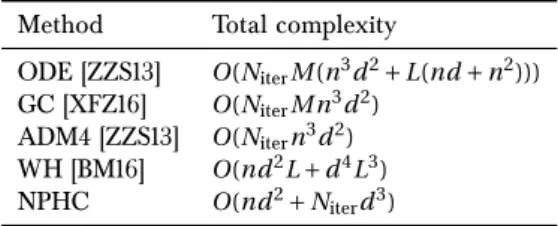
III Generalized Method of Moments approach 59 1 Introduction . . . 592 NPHC: The Non Parametric Hawkes Cumulant method . . . 62
2.1 Branching structure and Granger causality . . . 62
2.2 Integrated cumulants of the Hawkes process . . . 62
2.3 Estimation of the integrated cumulants . . . 64
2.4 The NPHC algorithm . . . 65
2.5 Complexity of the algorithm . . . 66
2.6 Theoretical guarantee: consistency . . . 67
3 Numerical Experiments . . . 68
4 Technical details . . . 73
4.1 Proof of Equation (8) . . . 73
4.2 Proof of Equation (9) . . . 73
4.3 Integrated cumulants estimators . . . 74
4.4 Choice of the scaling coe cient∑. . . 74
4.5 Proof of the Theorem . . . 75
5 Conclusion . . . 81
IV Constrained optimization approach 83 1 Introduction . . . 83
2 Problem setting . . . 83
3 ADMM . . . 85
Contents
3.2 Convergence results . . . 86
3.3 Examples . . . 86
4 Numerical results . . . 87
4.1 Simulated data . . . 87
4.2 Order book data . . . 87
5 Conclusion . . . 90
6 Technical details . . . 90
6.1 Convex hull of the orthogonal group . . . 90
6.2 Updates of ADMM steps . . . 90
Part III Capture order book dynamics with Hawkes processes
95
V Order book dynamics 97 1 Introduction . . . 972 Hawkes processes: deÆnitions and properties . . . 99
2.1 Multivariate Hawkes processes and the branching ratio matrixG . . . 99
2.2 Integrated Cumulants of Hawkes Process . . . 100
3 The NPHC method . . . 101
3.1 Estimation of the integrated cumulants . . . 101
3.2 The NPHC algorithm . . . 102
3.3 Numerical experiments . . . 103
4 Single-asset model . . . 104
4.1 Data . . . 104
4.2 Revising the 8-dimensional mono-asset model of [BJM16] : A sanity check . . . 106
4.3 A 12-dimensional mono-asset model . . . 107
5 Multi-asset model . . . 113
5.1 The DAX - EURO STOXX model . . . 113
5.2 Bobl - Bund . . . 115
6 Conclusion and prospects . . . 115
1 Origin of the scaling coe cient∑. . . 117
Bibliography 121 A Résumé des contributions 1 Résumé des contributions 1 Motivations . . . 1
Plan . . . 3
1 Part I: Modèle de Cox à grande échelle . . . 4
1.1 Contexte sur les algorithmes SGD, les processus ponctuels et le mod-èle des risques proportionnels de Cox . . . 5
2 Part II: Découvrir la causalité de Hawkes sans paramétrage . . . 9
2.1 Processus de Hawkes . . . 9
2.2 Approche par Méthode des Moments Généralisée . . . 10
2.3 Approche par optimisation sous contraintes . . . 12
3 Partie III: Capter la dynamique d’un carnet d’ordres à l’aide de processus de Hawkes . . . 13
3.1 Modèle 12-dimensionnel du carnet d’ordres d’un actif . . . 13
Introduction
The guiding principle of this thesis is to show how the arsenal of recent optimization methods can help solving challenging new estimation problems on events models. While the classical framework of supervised learning [HTF09] treat the observations as a collection of indepen-dent couples of features and labels, events models focus on arrival timestamps to extract information from the source of data. These timestamped events are chronologically ordered and can’t be regarded as independent. This mere statement motivates the use of a particular mathematical object called point process [DVJ07] to learn some patterns from events. Let us begin by presenting and motivating the questions on which we want to shed some light in this thesis.
Motivations
The amount of data being digitally collected and stored is vast and expanding rapidly. The use of predictive analytics that extract value of this data, often referred as the data revo-lution, has been successfully applied in astronomy [FB12], retail sales [MB+12] and search
engines [CCS12], among others. Healthcare institutions are now also relying on data to build customized and personalized treatment models using tools from survival analysis [MD13]. Medical research often aims at uncovering relationships between the patient’s covariates and the duration until a failure event (death or other adverse e ects) happen. The information that some patients did not die during the study is obviously relevant, but can’t be casted in a regression problem where one would need to observe the lifetime for all patients. This has been circumvented in [Dav72], one of the most cited scientiÆc paper of all time [VNMN14], with its proportional hazards model that is regarded as a regression that can also extract in-formation from censored data, i.e. patients whose failure time is not observed. An estimation procedure of the parameter vector of the regression without any assumption on the baseline hazard, regarded sometimes as a nuisance parameter, was introduced in [Cox75] and is done via the maximization of the partial likelihood of the model. Such procedure can e ciently handle high-dimensional covariates, which happens with biostatistics data, by adding penal-ization terms to the criterion to minimize [Goe10, Tib96]. However, algorithms to maximize Cox partial likelihood does not scale well when the number of patients is high, on the con-trary to most algorithms that enabled the data revolution. We might thus ask ourselves the following question:
Question 1. How to adapt Cox proportional hazards model regression parameter estimation
algo-rithm to the large-scale setting ?
Few years before the twentieth century, the French sociologist Durkheim already argued that human societies were like biological systems in that they were made up of interrelated com-ponents [Dur97]. Now that our technology enabled us to be remotely connected, plenty of Æelds involve networks, like social networks, information systems, marketing, epidemiology, national security, and others. A better understanding of those large real-world networks and processes that take place over them would have paramount applications in the mentioned domains [Rod13]. The observation of networks often reduces to noting when nodes of the network send a message, buy a product or get infected by a virus. We often observe where and when but not how and why messages are sent over a social network. Event data from multiple providers can however help uncovering the joint dynamics and revealing the un-derlying structure of a system. One way to recover the inØuence structure between di erent sources is to use a kind of point process named Hawkes process [Haw71b, Haw71a], whose arrival rate of events depend on the past events. Hawkes processes have been succesfully applied to model the mutual inØuence between earthquakes with di erent times and magni-tudes [Oga88]. Namely, it encodes how an earthquake increases the occurence’s probability of new earthquakes in the form of aftershocks, via the use of Hawkes kernels. Hawkes processes also enable measuring what we call Hawkes causality i.e. the average number of events of typei that are trigerred by events of type j. Hawkes process have been succesfully applied in a broad range of domains, the two main applications model interactions within social networks [BBH12, ZZS13, ISG13] and Ænancial transactions [BMM15]. However, usual estima-tion of Hawkes causality is done by making strong assumpestima-tions on the shape of the Hawkes kernels to simplify the inference algorithm [ZZS13]. A common assumption is the monotonic decreasing shape of the kernels (exponential or power-law), meaning that an event impact is always instantly maximal, which is non-realistic since in practice there may exist a delay before the maximal impact. This leads to the following question:
Question 2. Can we retrieve Hawkes causality without parametrizing the kernel functions ?
To answer positively to the second question, we developed two new nonparametric estimation methods for Hawkes causality, faster and which scales better with a large number of nodes. In this part, we only focus on the Ærst one, for which we have proved a consistency result. Since Bowsher’s pioneering work [Bow07], who recognized the Øexibility and the simplicity of using Hawkes processes in order to model the joint dynamics of trades and mid-price changes of the NYSE, Hawkes processes have steadily gained in popularity in the domain of high frequency Ænance, see [BMM15] for a review. Indeed, taking into account the irregular occurences of transaction data requires to consider it as a point process. Besides, in the Ænancial area, plenty of features that summarize empirical Ændings are already known. For instance, the Øow of trades is known to be autocorrelated and cross-correlated with price moves. Such features called stylized facts, from the economist Nicholas Kaldor [Kal57] who referred to statistical trends that need to be taken into account despite a possible lack of microscopic understanding. These stylized facts can advantageously be captured using the
Outline notion of Hawkes causality. Understanding the order book dynamics is one of the core ques-tion in Ænancial statistics, and previous nonparametric representaques-tions of order books with multivariate Hawkes processes were low-dimensional because of their estimation method’s complexity. The nonparametric estimation of Hawkes causality introduced in the second part of this thesis is fast and robust to kernel functions’ shape, and it is natural to wonder what kind of stylized facts it can uncover from order book timestamped data.
Question 3. Can we draw a more precise picture of order book Øows dynamics using Hawkes
causality’s nonparamatric estimation introduced in the second part ?
Outline
Each question presented above corresponds to a part of the thesis.
In Part I, we answer Question 1 by introducing a new stochastic gradient descent algorithm applied to the maximization of regularized Cox partial-likelihood, see details below. Indeed, the regularized Cox partial log-likelihood writes as a sum of subfunctions which depend on varying length sequences of observation, on the contrary to the usual empirical risk minimiza-tion framework where subfuncminimiza-tions depend on one observaminimiza-tion. Classical stochastic gradient descent algorithms are less e ective in our case. We adapt the algorithm SVRG [JZ13] [XZ14] by adding another sampling step: each subfunction’s gradient is estimated using a Monte Carlo Markov Chain (MCMC). Our algorithm achieves linear convergence once the number of MCMC iterations is bigger than an explicit lower bound. We illustrate the outperformance of our algorithm on survival datasets.
Answers to Question 2 lie in Part II where we study two nonparametric estimation procedures for Hawkes causality. Both methods are based on the computation of the integrated cumulants of the Hawkes process and taking advantage of relations between the integrated cumulants and the Hawkes causality matrix. The Ærst approach relies on matching the second and third order empirical integrated cumulants with their theoretical counterparts. This is done via the minimization of the squared norm of the di erence between the two terms, which can be viewed as a Generalized Method of Moments [Hal05]. However, the optimization problem to solve is non-convex providing thus an approximate solution to the exact initial problem. This second approach is based on the completion of the Hawkes causality matrix using the Ærst and second integrated cumulants. The relaxation of the exact problem writes as a convex opti-mization problem which enables us to provide the exact solution of this approximate problem. Finally, in Part III, we apply the Ærst method developed in Part II to high-frequency order book data from the EUREX exchange. We apply the procedure to Æt a 12-dimensional Hawkes order book model for a single asset and estimate the inØuence of the di erent events on each other. Such order book model is a natural extension of the 8-dimensional model studied in [BJM16]. We then scale the dimension so as to account for events of two assets simultaneously and discuss the joint dynamics and the cross-asset e ects. Usual nonparametric methods [BM14b]
[RBRGTM14] focus on the estimation of the kernel functions, and prevent order book model’s dimension from being too large and/or the dataset from being too heavy. Our nonparametric method only estimates kernels’ integral, involves a lighter computation and then scales better with a large number of nodes or large number of events. We also show that the Hawkes causality matrix provides a very rich summary of the system interactions. It can thus be a valuable tool in understanding the underlying structure of a system with many type of events. Let us now rapidly review the main results of this thesis.
1 Part I: Large-scale Cox model
Many supervised machine learning problems can be cast into the minimization of an ex-pected loss over a data distribution. Following the empirical risk minimization principle, the expected loss is approximated by an average of losses over training data, and a major success has been achieved by exploiting the sum-structure to design e cient stochastic algorithms [Bot10]. Such stochastic algorithms enable a very e cient extraction of value from massive data. Applying this to large-scale survival data, from biostatistics or economics, is of course of great importance.
In Chapter I, we review the recent advances in convex optimization with Stochastic Gradient Descent (SGD) algorithms, from the pioneering work of [RM51] to the recent variants with variance reduction [DBLJ14] [XZ14] [SSZ13] [RSB12]. We then introduce the notion of Point Process [DVJ07] which provides key tools for modeling events i.e. timestamps and/or locations data. We Ænally introduce the Cox proportional hazards model [Dav72] that relates the time that passes before some event occurs to one or more covariates via the notion of hazard rate. In Chapter II, we introduce our new optimization algorithm to help Ætting large-scale Cox model.
1.1 Background on SGD algorithms, Point Processes and Cox proportional
hazards model
In this chapter, we review the classic results behind Stochastic Gradient Descent algorithms and its variance reduced adaptations. We then introduce Cox proportional hazards model.
1.1.1 Stochastic Gradient Descent algorithms
SGD algorithms from a general distribution A variety of statistical and machine learning
optimization problems writes min
µ2RdF (µ) = f (µ) + h(µ) with f (µ) = E
ª[`(µ,ª)],
wheref is a goodness of Æt measure depending implicitly on some observed data,his a reg-ularization term that imposes structure to the solution andªis a random variable. Typically, f is a di erentiable function with a Lipschitz gradient, whereas h might be nonsmooth
-1. Part I: Large-scale Cox model typical examples include sparsity inducing penalty - such as the`1penalization.
First-order optimization algorithms are all variants of Gradient Descent (GD), which can be traced back to Cauchy [Cau47]. Starting at some initial pointµ0, this algorithm minimizes a di erentiable function f by iterating the following equation
µt+1= µt° ¥trf (µt). (1)
whererf (µ)stands for the gradient of f evaluated atµand(¥t)is a sequence of step sizes.
Stochastic Gradient Descent (SGD) algorithms focus on the case whererf is intractable or at least time-consuming to compute. Noticing thatrf (µ)writes as an expectation, one idea is to approximate the gradient in the update step (1) with a Monte Carlo Markov Chain [AFM17]. For instance, replacing the exact gradientrf (µ)with its MCMC estimate has enabled a sig-niÆcant step forward in training Undirected Graphical Models [Hin02] and Restricted Boltz-mann Machines [HS06]. This Ærst form of Stochastic Gradient Descent is called Contrastive Divergence in the mentionned contexts.
SGD Algorithms from the uniform distribution Most machine learning optimization
problems involve a data Ætting loss function f averaged over sample points because of the empirical risk minimization principle [Vap13]. Namely, the objective function writes
min µ2RdF (µ) = f (µ) + h(µ) with f (µ) = 1 n n X i =1 fi(µ),
wheren is the number of observations, and fi is the loss associated to the ith observation.
In that case, instead of running MCMC to approximate rf, one uniformly samples a ran-dom integer i between1 and n and replace rf (µ) with rfi(µ) in the update step (1). In
the large-scale setting, computingrf (µ)at each update step represents the bottleneck of the minimization algorithm, and SGD helps decreasing the computation time. Assuming that the computation of eachrfi(µ)costs1, the computation of the full gradientrf (µ) costsn,
meaning that SGD’s update step isntimes faster than GD’s one.
The comparison of the convergence rates is however di erent. Consider f twice di erentiable onRd,µ-strongly-convex, meaning that eigenvalues of the Hessian matrixr2f (µ)are greater thanµ> 0for anyµ2 Rd, andL-smooth, meaning that the same eigenvalues are smaller than L > 0. Convergence rates with other assumptions on the function f can be found in [B+15].
We denoteµ§ its minimizer and deÆne the condition number as ∑= L/µ. The convergence rate is deÆned for iterative methods as a tight upper bound of a pre-deÆned error, and is regarded as the speed at which the algorithm converges. Denotingµt the iterate aftertsteps of an iterative algorithm and considering the di erenceEf (µt) ° f (µ§)as error, Gradient
De-scent’s convergence rate is O(e°t/∑), while Stochastic Gradient Descent’s one is O(∑/t). A
convergence rate of the form O(e°Æt) with Æ> 0is called linear convergence rate since the
error decrease after one iteration is at worst linear. Equivalently, convergence rates can be phrased as the total complexity to reach a Æxed accuracy i.e. the number of iterations after
which the di erenceEf (µt) ° f (µ§)becomes smaller than≤> 0multiplied by the complexity
per iteration. The algorithm Gradient Descent will reach the accuracy≤afterO°∑log1≤¢ iter-ations resulting in aO°nd∑log1
≤
¢
complexity, while Stochastic Gradient Descent reachs such accuracy afterO°∑
≤
¢
iterations and then aO≥d∑≤ ¥complexity.
Recently, di erent works improved Stochastic Gradient Descent using variance reduction techniques from Monte Carlo methods. The idea is to add a control variate term to the descent direction to improve the bias-variance tradeo in the approximation of the real gradient rf (µ). Those variants also enjoy linear convergence rates, and then smaller complexities (to reach accuracy≤) than Gradient Descent since the complexity per iteration of those algorithms isO(d)versusO(nd)for Gradient Descent. Those typically typically enjoy complexity of the formO°(n + ∑)d log1≤
¢
in the strongly-convex case, see [SLRB17, JZ13, DBLJ14, SSZ13].
1.1.2 Point processes
Point process is a useful mathematical tool to describe phenomena occuring at random loca-tions and/or times. A point process is a random element whose values are point patterns on a setS. We present here the useful results when the setSis the interval[0,T ), and points are timestamps of events; this special case is sometimes called temporal point process. The book [DVJ07] is regarded as the main reference on point processes’ theory.
Every realization of a point process ª can be written as ª=Pni =1±ti where ± is the Dirac measure,n is an integer-valued random variable andti’s are random elements of [0,T ). It
can be equivalently represented by a counting processNt=R0tª(s)d s =Pni =11{ti∑t}. The usual characterization of temporal point process is done via the conditional intensity function, which is deÆned as the inÆnitesimal rate at which events are expected to occur aftert, given the history ofNs prior tot:
∏(t|Ft) = lim h!0
P(Nt+h° Nt= 1|Ft)
h ,
whereFt is the Æltration of the process that encodes information available up to (but not
including) the time t. The most simple temporal point process is the Poisson process which assumes that the events arrive at a constant rate, which corresponds to a constant instensity function ∏t= ∏ > 0. Note that temporal point processes can also be characterized by the
distribution of interevent times i.e. the duration between two consecutive events. We remind that the distribution of interevent times of a Poisson process with intensity∏is an exponential distribution of parameter∏. See the Page 41 of [DVJ07] for four equivalent ways of deÆning a temporal point process.
Two examples of temporal point process are treated in this thesis. The Ærst is the point process behind Cox proportional hazards model: its conditional intensity function allows to deÆne the hazard ratio, a fundamental quantity in survival analysis literature, see [ABGK12]. The Cox regression model relates the duration before an event called failure to some covariates. This model can be reformulated in the framework of point processes [ABGK12]. The second
1. Part I: Large-scale Cox model is the Hawkes process which models how past events increase the probability of future events. Its multivariate version enables encoding a notion of causality between the di erent nodes. We introduce below the Cox proportional hazards model, and the Hawkes processes in Part II.
1.1.3 Cox proportional hazards model
Survival analysis focuses on time-to-event data, such as the death in biological organisms and failure in mechanical systems, and is now widespread in a variety of domains like biometrics, econometrics and insurance. The variable we study is the waiting time until a well-deÆned event occurs, and the main goal of survival analysis is to link the covariates, or features, of a patient to its survival timeT.
Following the theory of point processes, we deÆne the intensity as the conditioned probability that a patient dies immediately aftert, given that he was alive beforet:
∏(t) = lim
h!0
P(t ∑ T ∑ t + h|t ∑ T )
h .
The most popular approach, for some reasons explained below, is Cox proportional hazards model [Dav72]. The Cox model assumes a semi-parametric form for the hazard ratio at time tfor the patienti, whose features are encoded in the vectorxi2 Rd:
∏i(t) = ∏0(t)exp(x>i µ),
where∏0(t)is a baseline hazard ratio, which can be regarded as the hazard ratio of a patient
whose covariates are x = 0. One estimation approach considers∏0 as a nuisance and only
estimatesµvia maximizing a partial likelihood [Dav72]. This way of estimating suits clinical studies where physicians are only interested in the e ects of the covariates encoded in x on the hazard ratio. This can be done with computing the ratio of hazard ratios from two di erent patients:
∏i(t)
∏j(t)= exp((xi° xj)
>µ)
For that reason, Cox model is said to be a proportional hazards model.
However, maximizing this partial likelihood is a hard problem when we deal with large-scale (meaning a large number of observations n) and high-dimensional (meaning large d) data. To tackle the high-dimensionality, sparse penalized approaches have been considered in the literature [Tib96] [T+97] [Goe10]. The problem is now to minimize the negative of the partial
log-likelihood f (µ) = °`(µ)with a penalizationh(µ)that makes the predictor µ to become sparse and then select variables. We will discuss this approach and the di erent models in Chapter II. On the contrary, approaches to tackle the large-scale side of the problem do not yet exist.
1.2 SVRG beyond Empirical Risk Minimization
Survival data(yi, xi,±i)i =1npat contains, for each individuali = 1,...,npat, a features vectorxi 2
Rd, an observed time yi2 R+, which is a failure time if±i = 1 or a right-censoring time if
±i= 0. IfD = {i : ±i= 1}is the set of patients for which a failure time is observed, ifn = |D|
is the total number of failure times, and ifRi= {j : yj∏ yi}is the index of individuals still at
risk at timeyi, the negative Cox partial log-likelihood writes
° `(µ) =n1 X i 2D h ° x>i µ+ log ≥ X j 2Ri exp(x>jµ)¥i (2)
for parametersµ2 Rd. Each gradient of the negative log-likelihood then writes as two nested expectations: one from an uniform distribution overD, the other over a Gibbs distribution, see Chapter II for details.
Our minimization algorithm is doubly stochastic in the sense that gradient steps are done using stochastic gradient descent (SGD) with variance reduction, and the inner expectations are approximated by a Monte Carlo Markov Chain (MCMC) algorithm. We derive conditions on the MCMC number of iterations guaranteeing convergence, and obtain a linear rate of convergence under strong convexity and a sublinear rate without this assumption.
2 Part II: Uncover Hawkes causality without parametrization
In Chapters III and IV, we study two methods to uncover causal relationships from a multi-variate point process. We focus on one approach per chapter.
2.1 Hawkes processes
In order to model the joint dynamics of several point processes (for example timestamps of messages sent by di erent users of a social network), we will consider the multidimensional Hawkes model, introduced in 1971 in [Haw71a] and [Haw71b], with cross-inØuences between the di erent processes. By deÆnition a family of d point processes is a multidimensional Hawkes process if the intensities of all of its components write as linear regressions over the past of thed processes:
∏it= µi+ D X k=1 Zt 0 ¡ i j(t ° s)dNj s.
Another way to construct Hawkes processes is to consider the following population represen-tation, see [HO74]: individuals of typei, 1 ∑ i ∑ d, arrive as a Poisson process of intensity µi. Every individual can have children of all types and the law of the children of typei of an individual of type j who was born or migrated int is an inhomogeneous Poisson process of intensity¡i j(· ° t).
2. Part II: Uncover Hawkes causality without parametrization This construction is nice because it yields a natural way to deÆne and measure the causality between events in the Hawkes model, where the integrals
gi j= Z+1
0 ¡
i j
(u) du ∏ 0 for 1 ∑ i, j ∑ d.
weight the directed relationships between individuals. Namely, introducing the counting func-tion Nti √j that counts the number of events of i whose direct ancestor is an event of j, we know from [BMM15] that
E[d Nti √j] = gi jE[d Ntj] = gi j§jd t, (3) where we introduced§i as the intensity expectation, satisfyingE[d Ni
t] = §id t. However in
practice, the Hawkes kernels are not directly measurable from the data and these measures of causality between the di erent kinds of events are thus inaccessible.
In the literature, there are main two classes of estimation procedures for Hawkes kernels: the parametric one and the nonparametric one. The Ærst one assumes a parametrization of the Hawkes kernels, the most usual assumes the kernels are decaying exponential, and estimate the parameter via the maximization of the Hawkes log-likelihood, see for example [BGM15] or [ZZS13]. The second one is based either on the numerical resolution of Wiener-Hopf equations which links the Hawkes kernels to its correlation structure [BM14b] (or equivalently on the approximation of the Hawkes process as an Autoregressive model and the resolution of Yule-Walker equations [EDD17]), or on a method of moments via the minimization of the contrast function deÆned in [RBRGTM14].
In Chapters III and IV, we propose two new nonparametric estimation methods to infer the integrals of the kernels using only the integrated moments of the multivariate Hawkes process. For all estimation procedures mentionned above, including ours, we need the following sta-bility condition so that the process admits a version with a stationary intensity:
Assumption 1. The spectral norm ofG = [gi j]satisÆes||G|| < 1.
2.2 Generalized Method of Moments approach
A recent work [JHR15] proved that the integrated cumulants of Hawkes processes can be expressed as functions ofG = [gi j], and provided the constructive method to obtain these
expressions. The Ærst approach we developed in this part is a moment matching method that Æts the second-order and the third-order integrated cumulants of the process. To that end, we have designed consistent estimators of the integrated Ærst, second and third cumulants of the Hawkes process. Their theoretical counterparts are polynomials ofR = (I °G)°1, as shown in
[JHR15]: §i= Xd m=1R i m µm Ci j= d X m=1 §mRi mRj m Ki j k= d X m=1 (Ri mRj mCkm+ Ri mCj mRkm+Ci mRj mRkm° 2§mRi mRj mRkm).
Once we observe the processNtfort 2 [0,T ], we compute the empirical integrated cumulants
on windows[°HT, HT], and minimize the squared di erenceLT between the theoretical
cu-mulants and the empirical ones. We have proven the consistency of our estimator in the limit T ! 1, once the sequence (HT)satisÆes some conditions. Our problem can be seen as a
Generalized Method of Moments [Hal05].
To prove the consistency of the empirical integrated cumulants, we need the following as-sumption:
Assumption 2. The sequence of integration domain’s half-length satisÆesHT! 1andHT2/T !
0.
We prove in Chaper III the following theorem of consistency.
Result 1. Under Assumptions 1 and 2, the sequence of estimators deÆned by the minimization of
LT(R)converges in probability to the true valueG:
b GT= I ° µ argmin R2£LT(R) ∂°1 P °°°°! T !1 G
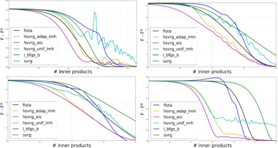
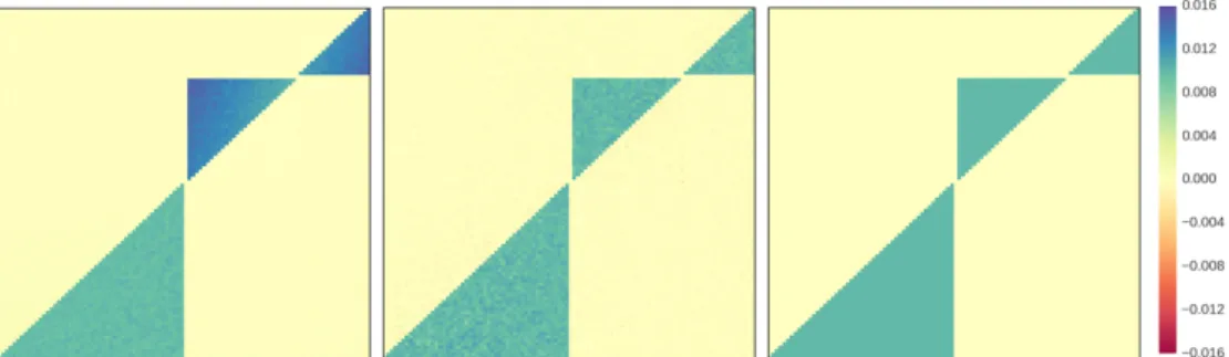
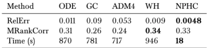
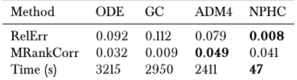
The numerical part, on both simulated and real-world datasets, gives very satisfying results. We Ærst simulated event data, using the thinning algorithm of [Oga81], with very di erent ker-nel shape - exponential, power law and rectangular - and recover the true value ofGfor each kind of kernel. Our method is, to the best of our knowledge, the most robust with respect to the shape of the kernels. We then ran our method on the 100 most cited websites of the MemeTracker database, and on Ænancial order book data: we outperformed state-of-the-art methods on MemeTracker and extracted nice and interpretable features from the Ænancial data. Let also mention that our method is signiÆcantly faster (roughly 50 times faster) since previous methods aim at estimating functions while we only focus on their integrals.
The simplicity of the method, that maps a list of list of timestamps to a causality map between the nodes, and its statistical consistency, incited us to design new point process models of order book and capture its dynamics. The features extracted using our method have very insightful economic interpretation. This is the main purpose of the Part III.
3. Part III: Capture order book dynamics with Hawkes processes
2.3 Constrained optimization approach
The previous approach based on the Generalized Method of Moments need the Ærst three cumulants to obtain enough information from the data to recover thed2entries ofG.
Assum-ing that the matrixGhas a certain structure, we can get rid of the third order cumulant and design another estimation method using only the Ærst two integrated cumulants. Plus, the resulting optimization problem is convex, on the contrary to the minimization ofLT above,
which enables the convergence to the global minimum. The matrix we want to estimate min-imize a simple criterion f convex, typically a norm, while being consistent with the Ærst two empirical integrated cumulants.
We formulate our problem as the following constrained optimization problem: min
G f (G)
s.t. C = (I °G)°1L(I °G>)°1 ||G|| < 1
gi j∏ 0
where f (G) is a norm that provides a particular structure to the solution. Every matrixG
satisfying C = (I ° G)°1L(I ° G>)°1 equals I ° L1/2MC°1/2 with M an orthogonal matrix.
Instead of the previous problem, we now focus on its convex relaxation, we split the variables
GandM, and solve the problem with the Alternating Direction Method of Multipliers algorithm, see [GM75] and [GM76]:
min
G,M f (G) + B(M) + B(G) + Rd£d+ (G)
s.t. G = I ° L1/2M C°1/2,
whereB (resp. B) is the open (resp. closed) unit ball w.r.t. the spectral norm. The closed unit ball w.r.t. the spectral norm is indeed the convex hull of the orthogonal group.
On the contrary to the optimization problem of the previous chapter, the problem just stated is convex. We test this procedure on numerical simulations of various Hawkes kernels and real order book data, and we show how the criterion f impact the matrices we retrieve.
3 Part III: Capture order book dynamics with Hawkes processes
Chapter V focus on the estimation of Hawkes kernels’ integrals on Ænancial data, using the estimation method introduced in Chapter III. This in turn allowed us to have a very precise picture of the high frequency order book dynamics. We used order book events associated with 4 very liquid assets from the EUREX exchange, namely DAX, EURO STOXX, Bund and Bobl future contracts.
3.1 A single asset 12-dimensional Hawkes order book model
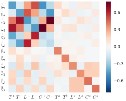
As a Ærst application of the procedure described in Chapter III, we consider the following 12-dimensional point process, a natural extension of the 8-12-dimensional point process introduced in [BJM16]:
Nt= (Tt+,Tt°,L+t,L°t,C+t,Ct°,Tta,Ttb,Lat,Lbt,Cta,Ctb)
where each dimension counts the number of events beforet:
• T+ (T°): upwards (downward) mid-price move triggered by a market order.
• L+ (L°): upwards (downward) mid-price move triggered by a limit order.
• C+(C°): upwards (downward) mid-price move triggered by a cancel order.
• Ta (Tb): market order at the ask (bid) that does not move the price.
• La (Lb): limit order at the ask (bid) that does not move the price.
• Ca (Cb): cancel order at the ask (bid) that does not move the price.
We then use the causal interpretation of Hawkes processes to interpret our solution as a measure of the causality between events. This application of the method to this new model revealed the di erent interactions that lead to the high-frequency price mean reversion, and those between liquidity takers and liquidity makers.
For instance, one observes the e ects ofT+ events on other events on Figure A.1 (in the Ærst
columnn on the left). The most relevant interactions are the T+! L+ and T+! L°: the
latter is more intense and related to the mean-reversion of the price. Indeedn when a market order consumes the liquidity available at the best ask, two main scenarios can occur for the mid-price to change again, either the consumed liquidity is replaced, reverting back the price (mean-reverting scenario, highly probable) or the price moves up again and a new best bid is created.
3.2 A multi-asset 16-dimensional Hawkes order book model
The nonparametric estimation method introduced in Chapter III allows a fast estimation for a nonparametric methodology. We then scale up the model so as to account for events on two assets simultaneously and unveil a precise structure of the high-frequency cross-asset dynamics. We consider a 16-dimensional model, made of two 8-dimensional models of the form
Nt= (P+t,P°t,Tta,Ttb,Lat,Lbt,Cta,Cbt)
where the dimensionP+ (P°) counts upwards (downward) mid-price move triggered by any
order.
We compared two couples of assets that share exposure to the same risk factors. The main empirical result of this study concerned the couple (DAX, EURO STOXX) for which price
3. Part III: Capture order book dynamics with Hawkes processes
Figure .1: Kernel norm matrixG estimated for the DAX future withH = 1s.
changes and liquidity changes on the DAX (small tick) mainly inØuence liquidity on the EURO STOXX (large tick), while price changes and liquidity changes on the EURO STOXX tend to trigger price moves on the DAX. We ran the estimation procedure on the 16-dimensional model, we focus our discussion on the two non-diagonal8£8submatrices on Figure A.2 that correspond to the interaction between the assets - the subscriptD stands for DAX andX for EURO STOXX.
The most striking feature emerging from Figure A.2 is the very intense relation between same-sign price movements on the two assets. Another notable aspect is the di erent e ects of price moves and liquidity changes of one asset on events on the other asset. Price moves on the DAX have also an e ect on the Øow of limit orders on EURO STOXX (P+
D! LbX
andP+
D! CXa), whereas EURO STOXX price moves triggers mainly DAX price moves in the
same direction (P+
X! PD+). An important aspect for understanding this result is the di erent
perceived tick sizes on the two assets. Note that the e ects observed above can be explained with the notion of latent price [RR10], see Chapter V for further details.
Figure .2: Submatrices of the Kernel norm matrixGcorresponding to the e ect of DAX events on EUROSTOXX STOXX events (left) and vice versa (right).
Part I
CHAPTER
I
Background on SGD algorithms, Point
Processes and Cox proportional hazards
model
1 SGD algorithms
Objectives that are decomposable as a sum of a number of terms come up often in applied mathematics and scientiÆc computing. They are particularly prevalent in machine learning applications, where one wants to minimize the average loss function over all observations. In the last two decades research on optimisation problems with a summation structure has focused more on the stochastic approximation setting, where the summation is assumed to be over an inÆnite set of terms [NJLS09, DS09, BCN16, Bot98]. The Ænite sum case has seen a resurgence in recent years after the discovery that there exist fast stochastic incremental gradient methods whose convergence rates are better deterministic Ærst order methods. We provide a survey of fast stochastic gradient methods in the later parts of this section.
1.1 DeÆnitions
In this work, we particularly focus on problems that have convex objectives. This is a major restriction, and one at the core of much of modern optimization theory. The primary rea-sons for targeting convex problems are their widespread use in applications and their relative ease of solving them. For convex problems, we can almost always establish theoretical re-sults giving a practical bound on the amount of computation time required to solve a given convex problem [NN94]. Convex optimisation is still of interest when addressing non-convex problems though: many algorithms that were developed for convex problems, motivated by their provably fast convergence have later been applied to non-convex problems with good empirical results [GBC16].
We denoterf the gradient of f,r2f its Hessian matrix and||·||the Eucliean norm. Let now deÆne some useful notions.
DeÆnition 1. A functionf isL-smooth withL > 0iff is di entiable and its gradient is Lipschitz continuous, that is
8µ,µ02 Rd, ||rf (µ) ° rf (µ0)|| ∑ L||µ ° µ0||.
If the functionf is twice di erentiable, the deÆnition can be equivalently written: 8µ 2 Rd, |eigenvalues[r2f (µ)]| ∑ L.
The other assumption we will sometimes make is that of strong convexity.
DeÆnition 2. A functionf isµ-strongly convex if:
8µ,µ02 Rd,8t 2 [0,1], f (tµ + (1 ° t)µ0) ∑ t f (µ) + (1 ° t)f (µ0) ° t(1 ° t)µ2||µ ° µ0||2. If f is di erentiable, the deÆnition can be equivalently written:
8µ,µ02 Rd, f (µ0) ∏ f (µ) + rf (µ)>(µ0° µ) +µ2||µ0° µ||2. If the functionf is twice di erentiable, the deÆnition can be equivalently written:
8µ 2 Rd, |eigenvalues[r2f (µ)]| ∏ µ.
Gradient descent based algorithms can be easily extended to non-di erentiable objectivesF if they write F (µ) = f (µ) + h(µ) with f convex and di erentiable, and h convex and non-di erentiable whose proximal operator is easy to compute.
DeÆnition 3. Given a convex functionh, we deÆne its proximal operator as
proxh(x) =argmin
y
∑ h(y) +1
2||x ° y||
2∏,
which is well-deÆned because of the strict convexity of the`2-norm.
The proximal operator can be seen as a generalization of the projection. Indeed, if h = 0 on C and h = 1 on C¯, proxh is exactly the projection over C. The computation of the proximal operator is also an optimization problem, but when the functionhis simple enough, the proximal operator has a closed form solution. Using these proximal operators, most algorithms enjoy the same theoretical convergence rates as if the objective was di erentiable (i.e.F (µ) = f (µ)).
1.2 SGD algorithms from a general distribution
A variety of statistical and machine learning optimization problems writes min
µ2RdF (µ) = f (µ) + h(µ) with f (µ) = E
1. SGD algorithms where f is a goodness of Æt measure depending implicitly on some observed data, h is a regularization term that imposes structure to the solution andªis a random variable. Typi-cally, f is a di erentiable function with a Lipschitz gradient, whereashmight be non-smooth (typical examples include sparsity inducing penalty).
First-order optimization algorithms are all variants of Gradient Descent (GD), which can be traced back to Cauchy [Cau47]. Starting at some initial point µ0, this algorithm minimizes a di erentiable function by iterating steps proportional to the negative of the gradient, as explained in Algorithm 1.
Algorithm 1 Gradient Descent (GD) initializeµ
while not converged do
µ√ µ ° ¥rf (µ)
end while returnµ
Stochastic Gradient Descent (SGD) algorithms focus on the case whererf is intractable or at least time-consuming to compute. Noticing that rf (µ)writes as an expectation like f, one idea is to approximate the gradient in the update step in Algorithm 1 with a Monte Carlo Markov Chain [AFM17]. Replacing the exact gradient rf (µ) with its MCMC estimate is a general approach that enabled a signiÆcant step forward in training Undirected Graphical Models [Hin02] and Restricted Boltzmann Machines [HS06]. This form of Stochastic Gradi-ent DescGradi-ent is called Contrastive Divergence in the mGradi-entionned context.
Approximating the gradient of an expectation, sometimes named the score function [CH79], is a recurrent task for many other problems. Among them, we can cite posterior computation in variational inference [RMW14], value function and policy learning in reinforcement learning [PB11], derivative pricing [BG96], inventory control in operation research [Fu06] and optimal transport theory [GM98].
1.3 SGD algorithms from a uniform distribution
Most machine learning optimization problems involve a data Ætting loss function f averaged over the uniform distribution, for instance when f is the average loss function over each observation of the data set. Namely, the optimization problem to solve writes
min µ2RdF (µ) = f (µ) + h(µ) with f (µ) = 1 n n X i =1 fi(µ),
wheren is the number of observations, and fi is the loss associated to the ith observation.
In that case, instead of running MCMC to approximaterf, one uniformly samples a random integer i between 1 andn and replace rf (µ) with rfi(µ)in the update step, as shown in
distribution case. In the large-scale setting, computingrf (µ)at each update step represents the bottleneck of the minimization algorithm, and SGD helps decreasing the computation time.
Algorithm 2 Stochastic Gradient Descent (SGD) initializeµas the zero vector
while not converged do
picki ª U [n] µ√ µ ° ¥rfi(µ)
end while returnµ
Assuming the computation of eachrfi(µ)costs1, the computation of the full gradientrf (µ)
costsn, meaning SGD’s update step isn times faster than GD’s one.
The comparison of the convergence rates is however di erent. Considerf L-smooth and con-vex and denoteµ§its minimizer. We deÆne the condition number∑= L/µ. The convergence rate is measured via the di erence f (µt) ° f (µ§). Using the algorithm Gradient Descent with
¥= 1/L, the convergence rates are: f (µt) ° f (µ§) ∑ O µ1 t ∂ , f (µt) ° f (µ§) ∑ O°e°t/∑¢ if f isµ-strongly convex.
The latter convergence rate which geometrically decrease the error is called linear convergence rate since the error decrease after one iteration is at worst linear. The convergence (in expectation) of the sequence (µt) produced by the algorithm Stochastic Gradient Descent
need the step sizes to decrease to zero a speciÆc way, see [RM51] for a general characterization. The convergence rate of stochastic algorithms is measured via the di erenceEf (µt) ° f (µ§).
Assuming each function fi is L-Lipschitz (and not L-smooth) and f is convex, denoting
µt=1tPtu=1µu, the convergence rates of Stochastic Gradient Descent are:
Ef (µt) ° f (µ§) ∑ Oµp1 t ∂ with ¥t= 1 Lpt, Ef (µt) ° f (µ§) ∑ O≥ ∑ t ¥ with ¥t= 1 µt if f isµ-strongly convex. Convergence rates with other assumptions on the function f can be found in [B+15]. Recently,
di erent works improved Stochastic Gradient Descent using variance reduction techniques from Monte Carlo methods. The idea is to add a control variate term to the descent direction to improve the bias-variance tradeo in the approximation of the real gradientrf (µ). Those variants also enjoy linear convergence rates with constant step-sizes.
1. SGD algorithms
1.4 SGD with Variance Reduction
The control variable is a variance reduction technique used in Monte Carlo methods [Gla13]. Its principle consists in estimating the population meanE(X )while reducing the variance of sample of X by using a sample from another variableY with known expectation. We deÆne a family of estimators
ZÆ= Æ(X ° Y ) + E(Y ) Æ2 [0,1],
whose expectation and variance equal
E(Za) = ÆE(X ) + (1 ° Æ)E(Y ),
V(Za) = Æ2[V(X ) + V(Y ) ° 2cov(X ,Y )].
The caseÆ= 1provides an unbiased estimator, while0 < Æ < 1implies ZÆto be biased with
reduced variance. This control variates is particularly useful whenY is positively correlated withX.
The authors of [JZ13] observed that the variance induced by SGD’s descent direction can only decrease to zero if decreasing step sizes are used, which prevents from linear convergence rate. In their work, they propose a variance reduction approach on the descent direction so as to use constant step sizes and obtain a linear convergence rate. The algorithms SAG [RSB12, SLRB17], SVRG [JZ13, XZ14], SAGA [DBLJ14] and SDCA [SSZ13] can be phrased with the variance reduction approach described above. Update steps of SAG, SAGA and SVRG withi ª U [n]respectively write this way:
(SAG) µ√ µ ° ¥ √ rfi(µ) ° yi n + 1 n n X j =1 yj ! , (SAGA) µ√ µ ° ¥ √ rfi(µ) ° yi+1 n n X j =1 yj ! , (SVRG) µ√ µ ° ¥ √ rfi(µ) ° rfi( ˜µ) +1 n n X j =1rf j( ˜µ) ! .
From the control variate interpreation, we observe that SAG’s descent direction is a biased estimate (Æ= 1/n) of the gradientrf (µ), while SAGA’s and SVRG’s ones are unbiased (Æ= 1).
Stochastic Average Gradient (SAG) At each iteration, the algorithm SAG [RSB12]
com-putes one gradient rfi with the up-to-date value of µ, like SGD, and then descend in the
direction of the average of the most recently computed gradientsrfj with equals weights, see
Algorithm 3. Even though some gradients in the summation haven’t been updated recently, the algorithm enjoys a linear convergence rate in the strongly-convex case. SAG can be re-garded as a stochastic version of Incremental Average Gradient [BHG07], which has the same update with a di erent constant factor, and with cyclic computation of the gradient instead of
randomised. The convergence rates in the convex and strongly-convex cases with¥= 1/(16L) respectively involves the average iterateµt and the iterateµt:
Ef (µt) ° f (µ§) ∑ O µ1 t ∂ Ef (µt) ° f (µ§) ∑ O≥e°t°8n1^16∑1 ¢¥ if f isµ-strongly convex.
The algorithm SAG is adaptative to the level of convexity of the problem, as it may be used with the same step size on both convex and strongly convex problems.
Algorithm 3 Stochastic Average Gradient (SAG) initializeµas the zero vector,yi= rfi(µ)for eachi
while not converged do
µ√ µ °n¥Pnj =1yj
picki ª U [n] yi√ rfi(µ)
end while returnµ
Stochastic Variance Reduced Gradient (SVRG) The SVRG algorithm [XZ14, JZ13] is a
recent stochastic gradient algorithm with variance reduction with linear convergence rate, given in Algorithm 4. Unlike SAG and SAGA, there is another parameterm to tune, which controls the update frequency of the control variate ˜µ. The algorithm S2GD [KR13] was developed at the same time, and has the same update as SVRG. The di erence lies in the update of the control variate ˜µ:
• Option I: ˜µis the average of theµvalues from the lastmiterations, used in [JZ13]. • Option II:˜µis a randomly sampledµfrom the lastmiterations, used for S2GD [KR13]. Consider f µ-strongly convex, a step size¥< 1/(2L), and assume m is su cently large so that
Ω= 1
µ¥(1 ° 2L¥)m+ 2L¥ 1 ° 2L¥< 1,
then the SVRG algorithm has a linear convergence rate ift is a multiple ofm: Ef ( ˜µt) ° f (µ§) ∑ O°Ωt/m¢.
Let us mention that SVRG does not require the storage of full gradients, on the contrary to SDCA, SAG and SAGA. The algorithm just stores the gradientrf ( ˜µ) and re-evaluates the gradientrfi( ˜µ)at each iteration.
1. SGD algorithms
Algorithm 4 Stochastic Variance Reduced Gradient (SVRG) initializeµand ˜µas zero vectors,t as zero
while not converged do
picki ª U [n]
µ√ µ ° ¥(rfi(µ) ° rfi( ˜µ) + rf ( ˜µ))
t √ t + 1
ift is a multiple ofmthen
update ˜µwith option I or II
end if end while returnµ
SAGA The algorithm SAGA [DBLJ14], described in Algorithm 5, enjoys a linear convergence
rate in the strongly convex case, like SAG and SVRG, but it has the advantage with respect to SAG that it allows non-smooth penalty terms such as `1 regularization. The proof of the
convergence rate is easier as well, especially because SAG’s descent direction is a biased esti-mate of the gradient, while SAGA’s one is unbiased. As SAG, the algorithm SAGA maintains the current iterateµand a table of historical gradients.
The convergence rate of the algorithm SAGA writes: Ef (µt) ° f (µ§) ∑ O≥ n t ¥ with ¥=3L1 , E||µt° µ§||2∑ O≥e°2(n+∑)t ¥ with ¥= 1 2(µn + L) if f isµ-strongly convex. Algorithm 5 SAGA
initializeµas the zero vector,yi= rfi(µ)for eachi
while not converged do
picki ª U [n] µ√ µ ° ¥≥rfi(µ) ° yi+1nPnj =1yj ¥ yi√ rfi(µ) end while returnµ
Composite case In the paragraphs above, we gave the convergence rates of the algorithm
in the smooth case i.e. when the objective function to minimize is a smooth function. When the objective function is not smooth, one writes it as the sum of its smooth part f (µ)and its non-smooth part h(µ). One can easily adapt the previous algorithms by computing the gradient of the smooth part f and then project the iterate using the proximal operator of the non-smooth part h. This adds a projection step µ√proxh(µ)at the end of each iteration.