THE EFFECTS OF SIZE AND PROPORTION OF RESIDU AL FOREST ON HARVESTING EFFORT AND HABITAT QUALITY INDEX OF THREE ANIMAL
SPECIES USING ECOSYSTEM BASED MANAGEMENT SCENARIOS IN BOREAL FOREST
THESIS
PRESENTED
IN PARTIAL REQUIREMENT OF
FOR THE MASTERS PROGRAM IN ENVIRONMENTAL SCIENCES
BY
JESSICA MARSHALL
Aved{sseaient
La diffusion de ce mémoire se fait dans lel respect des droits de son auteur, qui a signé le formulaire Autorisation de reproduire. et de diffuser un travail de recherche de cycles sup~rfeurs (SDU-522 - Rév.01-2006). Cette autorisation stipula qua ~~conformément à l'article 11 du Règlement no 8 dea études da cycles supérieurs, [l'auteur] concède à l'Université du Québec
à
Montréal une licence non exclusive d'utilisation et da . publlca'tlon da la totalité ou d'une partie importante de [son] travail da recherche pour dea fins pédagogiques at non commerciales. Plus précisément, [l'auteur] autorisa l'Université du Québec à Montréal à reproduira, diffuser, prêter, distribuer ou vendra des · copies de. [son] travail da rechercheà
des fins non commerciales sur quelque support qua ca soit, y compris l'Internet Cette licence et cette autorisation n'entrainent pas une renonciation de [la] part [de l'auteur}à [ses} droits moraux ni
à [ses] droits da propriété
intellectuelle. Sauf ententé contraire, [l'auteur} conserve la liberté da diffuser et da commercialiser ou non ce travail dont [il] possède un exemplaire .. »EFFETS DE LA TAILLE ET DE LA PROPORTION DE LA FORÊT RÉSIDUELLE
SUR L'EFFORT D'APPROVISIONNEMENT FORESTIER ET L'INDICE DE
QUALITÉ DE L'HABIT AT DE TROIS ESPÈCES ANIMALES SELON UNE
STRATÉGIE D'AMÉNAGEMENT ÉCOSYSTÉMIQUE EN FORÊT BOÉALE
MÉMOIRE
PRÉSENTÉ
COMME EXIGENCE PARTIELLE
DE LA MAÎTRISE EN SCIENCES DE L'ENVIRONNEMENT
PAR
JESSICA MARSHALL
I would like to start by thanking my supervisors. Osvaldo Valeria, who pushed me beyond my limits; for always demanding better, teaching me to be resourceful and for keeping your sense of humour during this ardent process, thank you! To Daniel Gagnon, if not for y our support, constant encouragement and advice, I would have given up long ago, thank you!
For their contributions to the computer models, thanks to Evan Hovington and Annie Belleau, without whose invaluable help I would have not made it through SELES.
Thanks to Melanie Desrochers and Ingrid Cea-Roa for their contributions to my training in ArcGIS. To Ingrid, whose friendship, constant help, and coffee maker made lem·ning GIS in Spanish until the wee hours of the morning enjoyable! For his last minute help in statistical analyses, thank you, Stéphane Daigle.
I would also like to thank the National Science and Engineering Council of Canada (NSERC), the Sustainable Forest Management Network (SFM Network) centres of Excellence (NCE) and the Roasters Foundation for their
financial support.
Finally, thank you to my parents for their support and unending encouragement, you're wonderful. And to my son Marcus, the reason I pursued my education.
LIST OF FIGURES ... .iv LIST OF TABLES ... v RÉSUMÉ ... vi ABSTRACT ... vii CHAPTER 1 GENERALINTRODUCTION ... 1
1.1 The emergence of ecosystem based forest management (EBM) ... 1
1.2 The theoretical framework behind EBM ... 2
1.3 Pilot projects adopted in Quebec to assess the acceptability and feasibility of EBM ... 3
1.4 The preindustrial fire portrait of north western region of Quebec ... 4
1.5 Residual forest patches found in naturallandscapes ... 5
1.6 Variable retention logging systems ... 7
1.7 The incorporation of spatial analyses in forest management and planning ... 9
1.8 Habitat quality index for selected regional fauna ... 10
1.9 Objectives ... 12
CHAPTERII METHODOLOGY ... 13
2.1 Modelling variable retention forest management scenarios based on EBM parameters ... 13
2.1.2 Study area ... 14
2.1.3 Residual forest parameters ... 14
2.2 Calcula ting the harvest effort of EBM variable retention scenarios ... 20 2.3 Calculating the habitat quality of EBM variable retention logging scenarios for three animal species ... 24
2.4 Correlation measurement analyses ... 26
CHAPTERIII RESULTS ... 28
3.2 Harvesting effort for variable retention logging scenarios based on EBM indicators ... 30 3.3 Impacts of retention patch types and other forest conditions on
harvesting effort ... 32 3.4 Impacts of retention patch types and other forest conditions on habitat
quality index for moose (Alces a/ces), marten (Martes americana), and hare (Lepus americanus) ... 33 CHAPTERIV
DISCUSSION ... 39 CHAPTER V
CONCLUSION ... 43 APPENDIXA
SELES PIRE MODEL... .... 45 APPENDIXB
SE LES VARIABLE RETENTION MODEL ... .46 REFERENCES ... 57
Figure 1.1
1.2
2.1
Page
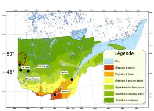
Location of the study area (north of La Sarre) and bioclimatic zones (Tembec, 2008) ... 4 The Rainboth Project: An example of a variable retention system
(Tembec,2008) ... 8
SELES retention event simulation of a 60000 ha site with minimum retention parameters (S5).
*
Peninulas- blue; Insular blocks- pink; Fragments- yellow ... 19 2.2 SELES retention event simulation of a 60000 ha site with maximumretention parameters (S6).
*
Peninulas- blue; Insular blocks- pink; Fragments- yellow ... 20 2.3 Variable retention harvest site of 60000 hectares with maximumretention (S6) ... 23 2.4 A habitat layer for a 60000 ha variable retention logging scenario
with maximum forest retention (S6).
*
Non-harvested forest (including retention)- dark green; Water-blue; Harvest blacks-brown; Wetlands- spotted green; Alder-light green; Dry lands-yellow ... 26 3.1 Average harvesting effort across scenarios ... 31 3.2 Proportion of habitat quality index across scenarios for moose (S1,S2 : 3000 ha ; S3, S4 : 15000 ha ; S5, S6 : 60000 ha) ... 34 3.3 Proportion of habitat quality across scenarios for marten (S1, S2:
3000 ha; S3, S4: 15 000 ha; S5, S6: 60 000 ha) ... 35
3.4 Proportion of habitat quality across scenarios for hare (S1, S2: 3000 ha; S3, S4: 15000 ha; S5, S6: 60000 ha) ... 35
2.1 2.2 2.3 2.4 3.1 3.2 3.3 3.4 3.5 3.6
Residu al forest parameters for dis turban ces of 3000 ha in size ... 16
Residu al forest parameters for perturbations of 15000 ha in size ... 17
Residu al forest parameters for perturbations of 60000 ha in size ... 17
Volume values for different Balsam fir, Pine, Spruce and Larch stands ... 23
Comparison of results of residual forest proportion in ha and percentage to our initial target parameters ac ross scenarios ... 29
Mean and SD across EBM scenarios ... 30
Average pre-existing kilometers of road for each scenario ... 32
Correlation measurements for harvest effort across scenarios ... 33
Correlation measurement test for moose habitat quality (Alces alces) ... 36
Correlation measurement test for marten habitat quality (Martes arnericanus) ... 37
3.7 Correlation measurement test for hare habitat quality (Lepus arnericanus) ... 37
3.8 Impacts of forest retention on harvesting effort and HQI for three animal species ... 38
La faune et la flore de la forêt boréale du Québec sont adaptées aux perturbations naturelles, plus particulièrement aux feux. L'approche écosystémique s'inspirant des dynamiques naturelles propose un avenir prometteur dans le développement des pratiques sylvicoles durables. Des études qui ont comparé les forêts résiduelles laissées par la récolte à celles laissées par les feux démontrent une différence significative entre la fréquence des îlots résiduels et leur configuration. Des différences qui ont probablement des impacts importants sur la faune et la flore de la région et sur 1' approvisionnement en bois. Six scénarios spatiaux avec 100 répétitions ont été simulés avec le logiciel SELES. Parmi ceux-ci, dix répétitions qui ont atteint nos cibles ont été sélectionnés selon différentes tailles (3000 ha, 15000 ha, et 60000 ha), fréquences et configurations pour évaluer leurs impacts sur l'effort d'approvisionnement. De plus, les effets environnementaux basés sur l'indice de qualité d'habitat pour l'Orignal (Alces alces), le lièvre d'Amérique (Lepus americanus) et la martre d'Amérique (Martes americana) ont également été évalués. Les résultats de ce projet permettent de faire des recommandations quant aux effets de la taille et de la proportion de la forêt résiduelle, selon différentes taille de chantiers de récolte, sur les efforts d'approvisionnement en forêt dominée par 1' épinette noire.
Mots clés: Épinette noire, aménagement écosystémique, taille des îlots résiduels, effort d'approvisionnement, qualité d'habitat.
The vegetation and wildlife of northern boreal forests in Quebec are adapted to natural disturbances, particularly wildfires. The ecosystem based management approach (EBM) is inspired by such natural dynamics and offers a promising avenue in the development of sustainable forestry practices. Previous studies examining the residual forest patches left by logging compared to those left by wiJdfires indicate that the shape of residual patches and patterns are significantly different and most probably have an impact on the wildlife of the region, as well as wood procurement efforts. Six spatial scenarios with one hundred repetitions each were simulated in SELES. The ten repetitions that best met our goals were then chosen in order to analyse the impacts of different residual patch size (3000 ha, 15000 ha, 60000 ha), frequency and spatial configuration on harvesting effort. In addition, environmental effects based on habitat quality index for moose (Alces a/ces), hare (Lepus americanus) and ma1ten (Martes americana) were also evaluated. The results of this project could help in the application of ecosystem based management approaches in black spruce dominated forests, while ensuring a certain level of conservation and biodiversity is maintained.
Key words: black spruce, ecosystem based management, residuaJ patch size, residuaJ patch frequency, harvesting effort, habitat quality index.
GENERAL INTRODUCTION
1.1 The emergence of ecosystem based forest management (EBM)
Since colonization, the forest industry has played an integral economie role in the province of Quebec (Linteau et al., 1983). Logging began in the province's Bas St-Laurent southern region and has since progressed northward. At the time, the premise was that once loggers reached the northern borders of the territory, the southern forests would have regenerated back to their original structure and composition. However, with the increase in market demands from growing populations and the ability to increase harvests through industrialization, forestry has now replaced natural disturbances as the primary stand-replacing force in the Canadian Boreal forests (Gauthier et al., 2008). In fact, Quebec's boreal forest is currently assessed to be the youngest it bas ever been throughout history (Bergeron et al., 2008). Furthermore, the development of ecological sciences bas explained why these presomptions regarding regeneration were far too simplistic when taking into account the complexity and diversity of forest ecosystems (Bergeron et al., 2008).
In the last two decades ecological knowledge as weil as socio-econornic shifts have changed the Canadian perception of the boreal forest (Perera et al., 2004). The large scale regeneration zones that were left by clear cutting and other Jogging practices became an increasing public concern with the arrivai of human activity in forested areas for recreational purposes. Communities have also been affected by forest activities. These are mainly First Nations communities, and their politics have also gained more public attention in recent years (Gauthier et al., 2008). In sum, the shift in perception is one of environmental concern. The elevated disturbance rates and large eut patterns caused by industrial forestry have created a discussion as to how we should manage our wood resources in order to maintain natural forest processes and patterns (Gauthier et al., 2008). Certain forest companies have also begun to respond to this environmental shift by modifying their practices to be environmentally
certified for international markets by the Forest Stewardship Council (FSC), Smart Wood or other certification organizations (Belleau et al., 2008).
A number of the environmental guidelines outlined by certification companies in
Quebec and other provinces in Canada (internationally as well) pertain to ecosystem based management approaches (EBM) (MRNFQ, 2009). Ecosystem management
approaches emerged in the forest sciences through the observations of forest disturbance regimes. Scientists from regions such as north western Quebec where
large natural disturbances are frequent became particularly interested in this phenomenon (Perera et al., 2004). According to Bergeron et al. (2002), a pioneer of
the ecosystem based management approach in Quebec, an EBM approach in the north-western boreal forests would be more cost effective and environmentally effective than restoring and managing the forests that have already been logged further South.
1.2 The theoretical framework behind EBM
Ecosystem based management is an adaptive approach to managing human activities
to ensure the coexistence of healthy, fully functioning ecosystems (Perera et al., 2004). EBM approaches are often rooted in the study of natural disturbances such as fires, diseases and insect epidemies. The main idea being that the vegetation and wildlife of forest regions are adapted to cyclic natural disturbances, th us, are part of a fully functioning ecosystem. The theory is that Jogging practices that are inspired by
natural disturbances would therefore cause Jess environmental degradation. The theoretical foundation of this approach is based on three key principles. The first being that (1) natural disturbances are recurrent within forest ecosystems at both
spatial and temporal scales, (2) that the vegetation and wildlife of these forest
ecosystems are adapted to the intrinsic disturbances of their environments and (3) that
a coarse filter approach to the conservation of biodiversity via forest management will maintain existing species (Franklin, 1993; MNRO, 2001).
---1.3 Pilot projects adopted in Quebec to assess the acceptability and feasibility of EBM
Even though values such as habitat quality, ecological processes and biodiversity are becoming increasingly important for global comrnunities and thus, forest industries, the application of EBM is still not well developed. One of the reasons is because it is a new concept that the provincial government has just adopted (MRNFQ, 2009). However, the lack of concrete guidelines also makes it increasingly difficult for forest industries to move away from their traditional practices towards new strategies when they still raise several questions including cost-effectiveness (Bergeron et al., 2002). Although previous studies conducted in Quebec have highlighted the importance of EBM indicators such as the composition, fragmentation and configuration of residual forests, the costs of their application are still undetermined. This project is part of one of three pilot projects being conducted in Quebec in order to improve, develop and validate tools for an evaluation of ecosystem based management approaches to allow us to assess its feasibility and acceptability. Since 2008, this project has been in the phase of moving from research to practice by creating a general plan for EBM on a designated forest management unit (FMU 85-51, see figure 1.1).
Érablière à bouleau jaune Sapinière à OOuleau jaune
Figure 1.1 Location of the study area (north of La Sarre) and bioclimatic zones (Tembec, 2008).
1.4 The preindustrial fire portrait of north western region of Quebec
The natural disturbance portrait of the north western regiOn of Quebec has been studied extensively. As a result, wildfires are now recognized as the primary natural
agent that has shaped the landscape and age structure of the forests over the past few
hundred years. The pre-industrial fire portrait of this area was created using archivai
data, air photos and fieldwork techniques in which the fire history for the past 300 years was reconstructed. The imprints left by fires on the landscape have allowed for the estimation of the fire cycle and the mean age of the forests, which is approximately 148 years old (Bergeron et al., 2002).
The pre-industrial fire portrait has also enabled the identification of fire sizes for the region. What we see is that the most frequent fires are less than 1000 ha, yet only
constitute 10% of the total forest burned (Bergeron et al., 2004 ). In the last sixty years, 55% of the total burned forest is a result of fire sizes ranging from 950 ha to 20 000 ha and the remaining 45% from fires greater than 20 000 ha (Bergeron et al.,
2002). The largest fires documented are approximately 67 000 ha (Bergeron et al., 2002).
Interestingly, these studies show that fires do not always have the severity to burn all
the trees in a site nor do they burn a site evenly (Belleau et al., 2008). For example,
10- 35 % of forest cover is left after a fire, and that 1 - 8 % of that quantity is found
in small islands of residual forests of 1 - 3 hectares. Also, that 30 - 50 % of affected
forest is only partially burnt. The knowledge that fire severity is variable within burns
implies major improvements should be made in the amount and configuration of
forest retention that should be left within harvested areas (Bergeron et al., 2002).
1.5 Residual forest patches found in naturallandscapes
The effects of fire severity create a variety of different spatial configurations of forest
retention patches that we do not see in harvested landscapes (Drapeau et al., 2002;
Dragotescu, 2008). For example, peninsular blocks, insular blocks, riparian strips,
and fragments are different types of retention patches seen in natural landscapes as
opposed to landscapes shaped by harvesting (Yelle et al., 2009). Studies on such
retention patches outline their benefits and the conditions needed within these patches for species maintenance. In addition to the studies conducted by Kafka et al. (2001),
Bergeron et al. (2002), Bennett (2003), Bergeron et al. (2007), and Y elle (2009) have
provided detailed descriptions of retention patches found in nature that can be used as
indicators in the application of EBM.
For instance, riparian strips are located in the moist areas along any body of water
and are commonly found after fire disturbances (Yelle et al., 2009). They play an
important role in the protection of aquatic ecosystems and are often very rich in
biodiversity. On the other hand, the insular block is important because it maintains interior forest conditions when it obtains a minimum of 250 meters in width with a size between 50 to 250 hectares (Yelle et al., 2009). Insular retention blacks are
advantageous for forest companies during the second harvest than eut separators in
agglomeration sites (Y elle et al., 2009).
Unlike the insular block, the peninsular block is a retention patch that stays connected
to a larger forest matrix. It plays an important role in connectivity, re-colonization
dynamics and minimizes edge effects by maintaining a good interior forest (Y elle et
al., 2009). In order to be effective, such peninsular retention patches must have 25 to
200 ha (Y elle et al., 2009). Peninsular blocks are also interesting at the financial and
operational level because they reduce road construction (Yelle et al., 2009). The
fragment or small island is also relevant to this study. Fragments are small retention
patches that are usually too small to contain an interior forest and are not as
interesting for species maintenance (Y elle et al., 2009) but can sometimes play a role
in connectivity.
Other studies show that important EBM indicators such as the shape, size and
fragmentation density of retention forest patches also vary by bioclimatic zones
(Perron, 2003; Dragotescu, 2008; Latrémouille, 2008). For example, the mean surface
area of retention forests after fire in the Northern Black Spruce domain was found to
be greater than that found in the Balsam Fir - White Birch domain. Therefore, bioclimatic information is pertinent in the development of forest management scenarios, and may be an issue for north western Quebec because it differs in
composition and structure from the south to the north of its territory.
Disturbances caused by wildfires were found to leave behind residual patch shapes
that are more complex than those left by Jogging (Perron, 2003). The retention
patches left by wildfires also appear to be smaller, doser in distance and more
frequent than those left by cuts (Dragotescu, 2008; Perron et al., 2008). These studies
highlight the importance of composition, fragmentation and configuration. All of which are influenced by fire severity and time (Gustafson, 1998).
1.6 Variable retention Jogging systems
Although it would appear that the incorporation of various types of forest retention patches cali for large modifications in Jogging techniques, other provinces have successfully proven otherwise. In 2002, the province of British Columbia adopted a variable retention system by using a combination of existing Jogging techniques (Mitchell et al., 2002). As a result, ranges in Jogging treatments from clear cutting, clear cutting with protection of regeneration and soils, to selection cutting can be used to mimic the range of effects found in natural disturbances. Bouchard (2008) also outlined different variable retention cuts that can be used in different stand and age structures. Even if the Jogging techniques used in British Columbia may not be applicable to Quebec, different species, species sizes and due to bioclimatic factors, the concept of variable retention system Jogging is promising. Figure 1.2 below shows a management scenario in a pilot project for Tembec Inc., known as the Rainboth site that was executed in 2007-2008. It is an example of an adaptation of variable retention systems for this region. The logging scenario is actually used to incorporate residual patches using an EBM strategy.
Chantier Rainooth 2007-2008 N Légende
A
CPRS - CPRS ovoc 251igoslho - CPRS por bouquots - Réteohon pertT'IôloenleBande riYoraine 5ans tôcole
- &ndo riveromo avoc rocollo
- Penklsule temporaire - Rètenhon lempOraire OH - Rolugos b"logiquoc - Alfos ProtCgées - Chomms B conslruiro - ChorTlnt 500 250 0 500 1000 , . . . . _ - 1 Métres 1 10 000
Figure 1.2 The Rainboth Project: An example of a variable retention system (Tembec, 2008).
In figure 1.2, dark green polygons represent permanent insular blocks and peninsula forest residuals, whereas the dark orange ones represent temporary insular blocks and peninsula forest residuals. The light orange polygons represent cutting with protection of regeneration and soils with a minimum retention of 25 trees per hectare while khaki green polygons represent the same eut with retention of clumps. The peach polygons represent cutting with protection of regeneration and soils (CPRS),
purple polygons representing biological refugia, and blue polygons are protected areas (Tembec, 2008).
For instance, in figure 1.2, the retention variability mimics the effect that only 30-50 % of stands are partial! y burnt in an area affected by wildfires (Bergeron et al., 2002). These variable retention techniques also promote a more complex future stand
structure that contains more dead wood, provides shelter for species with reduced dispersion capacity and for species that frequent the affected area, promotes habitat
diversity and ecological processes linked to soil productivity (Tembec, 2008). In addition, within the site, permanent and temporary peninsular and insular residual blacks are retained, as well as partially harvested and untouched riparian strips.
1.7 The incorporation of spatial analyses in forest management and planning
With the evolution of technology, new complex software programs can now help answer increasingly complex spatial questions in forest management and planning. Spatial analyses at the disturbance-scale can offer the incorporation of more detailed operational planning possibly reducing costs and off site impacts (MacDonald et al., 2000). There are several spatial tools available for such planning such as LANDIS, Patchworks and SELES among others. SELES software is particularly effective for exploring the effects of wildfires on landscape structures at the disturbance-scale (FaU et al., 2008). In addition, SELES is not designed for particular landscape types, or sets of processes, thus each madel requires detailed parameterization for modelling different scenarios (Fall et al., 2008).
Advancement in GIS technology now makes it possible to detect and characterize large-scale temporal changes of multiple forest attributes (Baskent and Yolasigmaz, 1999). Recent studies in landscape and conservation ecology have shawn that ecological considerations and their spatial context should be taken into account in the planning and management of forest resources (Galindo-Leal and Bunnell, 1995; Baskent and Yolasigmaz, 1999). Forest landscape history (according to its spatial characteristics) can be deduced from forest inventories produced from aerial photographs or satellite imagery (Pas tor and Broschart, 1990; Ripple et al., 1991 ). Hence, spatial characteristics of stands can be used as a basis to establish management objectives (e.g., size of regeneration areas). Such an approach in planning, where the structure and composition of the landscape is taken into account, has been used in severa! American national forests, where managers recognize the
1.8 Habitat quality index for selected regional fauna
Originally, in Québec, measures were put forth for the protection of animal species themselves. The need to also protect animal habitats became more and more evident starting in the second half of the 20th century. This corresponds to the shift to coarse filter approaches by the Ministry of Natural Resources and Fauna. Species that inhabit north western Quebec require a unique habitat which should be taken into consideration under forest operations. lt is important to monitor these focal species (indicator and vulnerable species) arnidst anthropogenic activities in order to determine the health of the ecosystem.
One of the boreal regions focal species is the moose (Alces alces). Moose tend to inhabit forested areas with young leafy trees or mixed forests near sources of water during summer months (Courtois, 1993; FEIS, 2009). Then when the climate cools in winter months, they move to denser, coniferous forests (FEIS, 2009). Moose actually prefer areas that have recently been disturbed, which make it one of the less vulnerable species of the Abitibi region (Courtois, 1993). Therefore, cuts with protection of soil and regeneration (CPRS) with various retention and insular and peninsular blocks may be favourable for this species, as it could incorporate both the dense coniferous and younger vegetation with which it is associated. However, re -colonization of this species in a disturbed area rarely takes place before 5-6years after disturbance (Caners et al., 2008). In 1993, Courtois identified 5 main variables to determine habitat quality index:
1) An abundant and diversified terrestrial food chain (leaves and deciduous twigs)
2) Access to wetlands (aquatic food, thermal regulation in summer).
3) Flight cover (forest that is less harvested to reduce loss due to hunting and predation).
4) Coniferous protection cover (favoured for thermal regulation at the end of the winter, rninirnizes energy loss).
5) Specifie habitats (saline, calving grounds, etc.).
These diverse variables must intermingle in order to minimize displacement and to
permit optimal grazing, rest and ruminating (Bas St-Laurent Forest Mode! Network,
2003).
The snowshoe hare (Lepus americanus) is another focal species. It is larger than a rabbit and is associated with the edge of residual forests and, similar to the moose,
disturbed areas (Monthey, 1986). They prefer a mix of deciduous and coniferous
forests for food sources (Guay, 1994) and survive in a smaller home range of
approximately 10 ha or Jess (Guay, 1994). Forests with Jess than 60% cover which
permit a denser undergrowth to establish is a necessity for protection against
predators (Orr and Dodds, 1982). According to Guay (1994), two parameters are
important in habitat quality for this species; (1) the IQHP indicator which calculates
the quality of the stand and (2) the IQHÉ indicator which calculates the quality of the
eco-tone corresponding to the edge effect between two stands.
The american marten is another focal boreal species mentioned in this thesis. It is a
long, slender-bodied weasel about the size of a mink with relatively large rounded
ears, short limbs, and a bushy tai!. A study in the Abitibi region by Potvin et al. (2000) identified that the american marten (Martes americana), avoided recently
disturbed areas. Due to the fact that 80% of a marten's diet is animal prey (mice,
voles) they spend mu ch of the ir time foraging for food both in trees and on the forest
floor. Potvin et al. (2000) clearly identifies this mammal with mature forests and a
need of a forest cover that lasts over 30 years which signifies that permanent residual
blocks (peninsular and insular) and forest massifs may be necessary to maintain this species. According to Larue (1992), the main habitat criteria for marten is based on (1) the composition and density of conifers (CEDC), (2) the developmental stage of the forest (SDEVEL), and (3) stand height and wood debris (DLIGNEUX). The model is expressed by the equation: the cubic root of the dividend of the product of CEDC, SDEVEL and DLIGNEUX divided by three.
1.9 Objectives
The general objective of this project is to create a spatial model in arder to evaluate different EBM forest retention scenarios to measure harvesting effort ((m3/ha*total ha) 1 total km) and habitat quality index for three animal species. Based on the aforementioned literature, we expect that the greater percentage of residual forests will result in lower harvesting efforts (higher cost estimates) and stronger habitat quality (Perron, 2003, Y elle et al., 2009, Bennett, 2003). However, we would like to
test the effects of the patch type, frequency and proportion on estimation of harvesting effort and habitat quality index for moose, marten and hare. In sum, this
study is driven by three main objectives:
1) To create a model that can generate variable retention scenarios inspired by wildfire.
2) To calculate the harvesting effort of variable retention Jogging scenarios based on retention indicators from ecosystem based management studies.
3) To calculate the habitat quality index found in our generated variable retention Jogging scenarios for three focal boreal animal species.
2.1 Modelling variable retention forest management scenarios based on EBM parameters
SELES (Spatially Explicit Landscape Event Simulator) is a model building and
simulation tool that attempts to strike a balance between the flexibility of
programming languages to construct novel models and the ease of applying and
parameterizing pre-existing models. SELES models have been successfully applied to
support forest landscape decision processes for land-use planning (north coast of
Quebec, Haïda Gwaii and Mariee area,s in B.C.), natural disturbance management
(mountain pine beetle, fires), sustainable forest management planning (upper Mauricie area of Quebec), recovery plans for species at risk (Spotted Owl), habitat connectivity (woodland caribou), and parks planning (www.seles.info). It is useful as a research tool as well as a decision-support tool for management, and for problems
related to both conservation and resource management (FaU, 2012).
Our goal was to use SELES to create variable retention scenarios based on ecosystem
based forest retention management parameters for further assessment. There are no
specifie data requirements or limits for SELES. All spatial data must have the same extent and resolution. Inputs can include spatial raster (grid) data (e.g. species, stand age), tables (e.g. volume curves) and parameters (e.g. fire rotation). We were able to
build upon an existing fire model by incorporating residual parameters so simulations
mimicked wi1dfire. The following data were required for our models: (1) eco-forest map of our study area, (2) size of logging sites inspired by wildfire, (3) a pre-industrial fire model of our study area, and ( 4) forest retention parameters.
2.1.2 Study area
Our study area is the forest management unit 85-51 (FMU), located in the mid-western area of the province of Quebec known as the Abitibi region (see figure 1.1). Tembec also shares the management responsibilities of this unit with Norbord industries, another forest company interested in an ecosystems approach. FMU 85-51 extends from latitudes 49'00'- 51'30' N and longitudes 78'30'- 79'31 W. It covers a surface are a of 10 826 km2 of the 6a- Matagami ecological region in the western extremity of the black spruce feathermoss bioclimatic domain. This is the sub-region of Quebec's boreal forest, dominated by black spruce (Picea mariana Mill), jack pine
(Pinus banksiana Lamb), and trembling aspen (Populus tremuloides Michx). The annual average temperature for this region is -0.7
c
o
and the annual precipitation is approximately 905 mm. The region is also characterized by clay soil types, a result of the areas post glacial lakes (Belleau and Légaré, 2008). There are a few inhabitants on its territory but it is still frequented by First Nations people, hunters, fishermen, trappers, vacationers, workers, miners and loggers (Tembec, 2008).2.1.3 Residual forest parameters
In order to create scenarios of different forest residual patches based on EBM indicators, logging site sizes were set according to the mean wildfire sizes identified in the pre-industrial fire portrait for our study area (Belleau et al., 2007). Small fires of 3000 ha, medium size fires of 15 000 ha and large fires of 60 000 ha. Data regarding different residual forest patch quantity inspired by wildfire were then grouped in accordance to disturbance size (Kafka et al., 2001; Bergeron et al., 2002;
Bennett, 2003; Perron, 2003; Bergeron et a/.,2007; Dragotescu, 2008; Latrémouille, 2008; Yelle et al., 2009) The aim was to create multiple stochastic residual forest patch patterns, shapes and sizes, found in natural landscapes including fragments (small islands), insular blocks, peninsular blocks and riparian strips depending on the size of the disturbance sites being analyzed while remaining within a set of
parameters in order to eventually test the effects of residual forest gradients and size on harvesting effort and habitat quality index.
Total residual forest
Bergeron (2008) found that a mean of 5 % of total residual forests were found after
fire in Quebec's black spruce dominated Boreal forests, however fire size was not
mentioned. Because Quebec's black spruce dominated forests are mostly dominated
by small fires of 1000 hectares or less the 5 percent total residual forests deducted by
Bergeron (2008) most probably reflects the higher frequency of smaller fires (Perron,
2003). Also, according to Eberhardt and Woodard (1987), from a study of 69 Boreal
forest fires in Alberta, a maximum value of 18 % for total residual forests was found after fire and the fires ranged in size from 21 to 17 770 ha for this study. Therefore, in
order to include residual forests for fires of 60000 ha, the parameter values have been
regrouped to 3-6 %, 12-15 % and 19-22 % total residual forests for fires of 3000,
15000 and 60000 ha respectively (see tables 2.1 to 2.3).
Fragments
According to Perron (2003), 0 to 8 % of total residual forests was found in isolated
small islands of 1-3 ha called fragments in fires of up to 35000 ha in black spruce forests. Therefore, in order to omit the percentage of fragments created by fires less than 3000 ha and incorporate fi res of 60000 ha a range of values between 2-13 %
residual forests in the form of fragments was used (see tables 2.1 to 2.3). The total
density of patches ranged from 7 to 37 patches per 100 ha.
Insu/ar and peninsular blocks
The data on insular blocks is much simpler. In order to be maintain mammal and bird
species a surface area of 50 to 250 ha of forest must remain (Tembec, 2008; Y elle et al., 2009). Peninsular residual patches, which are connected to a forest matrix, must
be 25 to 200 ha or more than 500 rn long to play a positive role in connectivity and
The values from these previous studies were divided into two groups in order to represent A) the minimum retention values and B) the maximum retention values
according to disturbance size (see tables 2.1 to 2.3). Because the range in total residual percentages is relatively small, the mean values have been omitted in order to measure a clear difference in variability. Therefore, six different simulations were generated for scenarios A and B for all three fire sizes with ten repetitions each to complete a total of sixty different EBM forest management scenarios. The scenarios are grouped as follows: (S 1) represents minimum and (S2) the maximum retention values for perturbations sites of 3000 ha in size; (S3) represents the mini!llum and (S4) represents the maximum retention values for sites 15000 ha in size; (S5) represents the minimum and (S6) the maximum retention values for sites 60000 ha in
size. In addition, the percentage allocated to insular and peninsular blocks are 50/50,
an equal division between each. Based on the modified residual forest values mentioned above, that was used to evaluate forest residual management for disturbances of 3000 ha are as follows. ( 1) S 1 consists of 3 % total residu al forests
including 1% of that forest under the form of fragments and the remaining 2 % under the form of insular blocks (50 ha) and peninsular blocks (25 ha). S2 consists of 6 %
total residual forests with 4 % of fragments, with maximum values for insular blocks
of 110 ha and peninsular blocks of 70 ha (see table 2.1 for model inputs).
Table 2.1 Residual forest parameters for disturbances of 3000 ha in size
Scenarios* Total residual forest Fragments Insular blocks Peninsular blocks
Sl 3% 1% 50 ha 25 ha
S2 6% 4% 110 ha 70 ha
*S 1= minimum EA value and S2= maximum EA value
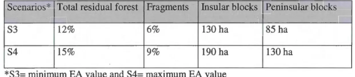
The modified residual forest values mentioned above, that were used to evaluate forest residual management for disturbances of 15000 ha are as follows. S3 consists
of 12% total residual forests with 6 % under the form of fragments (1 to 3 hectares in
size) and the remaining 6 % in insular blocks with a minimum value of 130 ha and
forests with 9% fragments and the remaining insular blocks of 190 ha and peninsular blocks of 130 ha (see table 2.2 for model inputs).
Table 2.2 Residual forest parameters for perturbations of 15000 ha in size
Scenarios* Total residual forest Fragments Insular blocks Peninsular blocks
S3 12% 6% 130 ha 85 ha
S4 15% 9% 190 ha 130 ha
*S3= minimum EA value and S4= maximum EA value
The modified residual forest values that were used to evaluate forest residual management for disturbances of 60000 ha in size are as follows. S5 consists of 19 % total residual forests with 10 % under the form of fragments and the remaining 9 % under the form of insular blocks with minimum values of 190 ha and peninsular blocks of 145 ha. S6 consists of 22 percent total residual forests with 13 % found in fragments and the remaining 9 % in insular blocks with maximum values of 250 ha and peninsular blocks of 200 ha (see table 2.3 for model inputs).
Table 2.3 Residual forest parameters for perturbations of 60000 ha in size
Scenarios* Total residual forest Fragments Insular blocks Peninsular blocks
S5 19% 10% 190 ha 145 ha
S6 22% 13% 250 ha 200ha
*S5= minimum EA value and S6=.maximum EA value
In order to accomplish the desired forest residual scenarios in SELES, two models and two sub models were used: a disturbance mode], a retention mode], a buffer sub model and the Filter Small sub model. (1) A fire model developed by Annie Belleau was adjusted and used as a landscape disturbance model, emulating a Jogging site shape resembling that of one left by wildfire according to site size parameters (3000 ha, 15000 ha, 60000 ha). (2) The Filter Small sub model, from SELES model garden (www.seles.info), was then used to find unaccounted pixels within the site and delete them. These pixels are representative of areas left un-burnt by wildfire but would
have skewed our set forest residual parameters, increasing the sum and size of fragments, blocks and peninsulas significantly. (3) In order to simulate peninsulas, a buffer sub model was used. A buffer was simulated within the disturbance close to the edge of its perimeter. This created an area in which to run the retention model for peninsulas to ensure these residual patches were attached to the larger forest matrix and thus act as a corridor for species. Another buffer was then simulated close to the edge of the first buffer to separate the area in which to run the retention model for insular blocks and fragments to ensure that they didn't attach themselves to the peninsulas and skew set parameters. ( 4) A residu al model was created using the
aforementioned fire model, to ensure residuals also resembled wildfire with the
incorporation of our aforementioned residu al parameters for our scenarios (S 1, S2, S3, S4, S5, and S6) (See appendix for scripts).
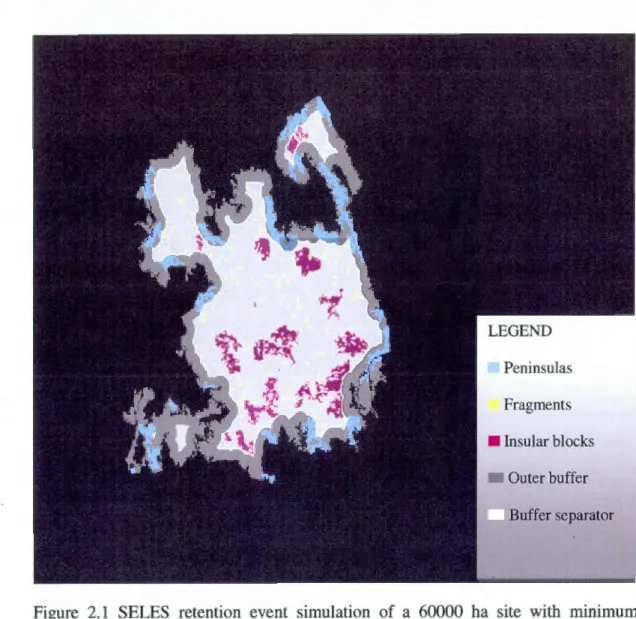
Output data was classified as follows for each residual patch type by colour; peninsulas-blue, insular blocks-pink and fragments-yellow. Figure2.1 represents an example of a scenario containing the minimum residual forest within a harvest site of 60000 ha (S5). It contains 30 insular blocks with a surface area of 5095 ha, 300 fragments with a surface area of 658 ha and 49 peninsulas with a surface area of 4938 ha. The total amount of planned residual forest in this site is 10691 ha. The first buffer zone is dark gray and is where the blue peninsulas are located. The second buffer zone is white and separates the insular blocks and fragments from peninsulas. In total, ten repetitions of each scenario (S1, S2, S3, S4, S5, and S6) were chosen.
Peninsulas Fragments
Figure 2.1 SELES retention event simulation of a 60000 ha site with rrummum
retention parameters (S5).
*
Peninsulas- blue; Insular blocks- pink;Fragments-yellow
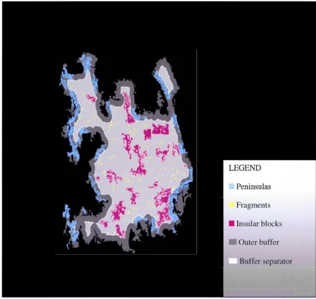
Another example is Figure 2.2 that represents a scenario containing the maximum residual forest within a harvest site of 60 000 ha (S6). It contains 30 insular blocks
with a surface area of 5972 ha (pink), 299 fragments with a surface area of 688 ha
and 50 peninsulas with a surface area of 6323 ha. The amount of total planned
residual forest for this site is 12 983 ha. Once again, the first buffer zone is dark gray
and is where the blue peninsulas are located. The second buffer zone is white and
Peninsulas Fragments
Figure 2.2 SELES retention event simulation of a 60000 ha site with maximum
retention parameters (S6).* Peninsulas- blue; lnsular blocks- pink; Fragments- yellow
2.2 Calculating the harvest effort of EBM variable retention scenarios
All sixty chosen SELES retention simulation scenarios were transformed from raster file into vector format (polygons) to be transferred to ArcGIS® in order to create variable retention Jogging scenarios. Two spatial input shape files or feature classes were required to obtain a ratio for harvesting effort: (1) a harvest layer (including planned harvest blocks, the surface area harvested (ha), the tree species, age, height and coverage densities of planned logged forest stands) and (2) a road layer
(including the length in km of the road networks constructed to access planned eut blocks).
Eco-forest maps (classification maps that include detailed ecological information for a region) from the provincial government (1995) were over-layed in ArcGIS in order to identify the forested areas, stand types, vegetation types, location of water sources, wetlands, barren lands and other important geographical information, surrounding simulated residual forest patches. Eco-forest maps were essential in the identification of productive forest tree species (Fir, Pine, Spruce and Larch) (Belley, 2002), stand age (90 to 120 years old), stand heights 7 to 22 rn (Class 2,3,4) and coverage density of 25 to 80 % (Class B, C, D) (Directions des Inventaires Forestiers, 2009). Once the timber-productive forest was identified, a potential harvest layer was created. Buffers of 20 rn were incorporated around water sources and residual forests in order to ensure their ecological integrity.
Road networks were created in ArcGIS within the potential harvest layer. Secondary and tertiary roads were created from a starting point (camp) that connected to a major road outside of planned logging sites. All roads were modeied to the minimum specifications required to transport harvested wood, while protecting the environment, therefore, networks that demanded the least road construction were favoured. Road networks followed the general road construction principles; leaving a minimum of 1 km between roads for harvesting machinery that operate up to 500 rn on both sides of a road (MRNFQ, 2009). Once the road networks were set, a buffer of 500 rn was created around the roads in order to determine the accessible potential harvest area. Timber-productive forest within this buffer became planned eut blocks. Cut blacks represented approximately 80 % or more of available timber-productive forests across scenarios.
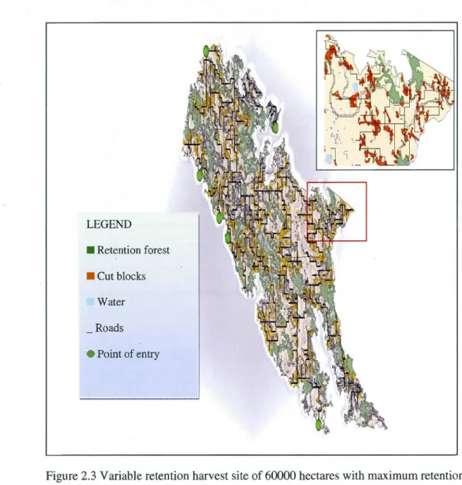
Figure 2.3 shows a 60 000 ha variable retention Jogging scenario with the maximum forest residual parameters, created in ArcGIS from S6. This scenario size is 68325 ha. The green polygons representa total of planned residual forests of 12456 ha of which 30 polygons are insular blocks (4662 ha), 300 polygons are fragments (736 ha), and
49 polygons are peninsulas (5640 ha). However, the total amount of non-harvested
forest which includes both productive and non-productive forest is 16725 ha. The
orange polygons represent harvest blocks consisting of 6925 hectares of harvested productive forest. The black polylines represent the planned road network with a total
of 521 km in length and the lime green circles represent points of entry or camps. An
attribute table is incorporated to every layer in each map. The tables include information pertaining to each forest stand (height, coverage density, age, tree
species, other vegetation types, and landscape types) needed in order to calculate volumes for harvesting effort ratio ((m3/ha*total ha)/total km)). The smaller image in
the upper right corner of figure 2.3 is a close up of an area within this logging site.
The eco-forest map layer for the region was used in order to identify the different
volumes for each harvest block by polygon in a logging site. This is an important
aspect of the effort estimation because differences in volume values and road access
length represent different effects on wood procurement cost (see table 2.4). These
estimations were based on basic stand data used in forestry in Quebec (MRNFQ, 2009) and were validated with a Tembec manager and considered a good approximation. Once the volumes were associated to planned eut blocks, an effort ratio was calculated (m3/ha * total ha)/total km in ArcGIS. The ratio is an estimation
of the harvesting· effort of each EBM variable retention Jogging scenario in order to determine cost-effectiveness. The assomption is that as harvesting effort decreases,
LEGEND • Retention forest • eut blocks Water Roads
e
Point of entryFigure 2.3 Variable retention harvest site of 60000 hectares with maximum retention (S6) *Retention forest-green; Cut blocks-orange; Water-blue; Roads-black polyline; Points of entry-green circles.
Table 2.4 Volume values for different Balsam fir, Pine, Spruce and Larch stands attributes.
Density Age Height m3/ha
40-80% > 90 12-22 rn 114
40-80% >or=120 12-22 rn 89
2.3 Calculating the habitat quality of EBM variable retention logging scenarios for three animal species
Ail sixty variable retention Jogging scenarios were evaluated individually in relation to environmental conditions associated with moose (Alces alces), snowshoe hare (Lepus americanus), and marten (Martes americana) using the Habitat Quality Index or "Indices de Qualité d'Habitat (IQH)" extension in ArcView version 3.0 (Bas St-Laurent Forest Model Network, 2003). The extension calculates habitat quality based on specifie habitat quality index models for various species as weil as geographical attributes corresponding to the third decadal provincial timber inventory.
In order to transfer the variable retention Jogging scenarios to the habitat quality index extension 3.0 in ArcView, a habitat layer was created. A union between the eco-forest map layer and the harvest layer was executed to create a layer cailed habitat. Polygons belonging to the harvest layer, eut blocks, were modified in order to analyze the harvest site post cuts. In the extension, the model for moose is based on the Courtois (1993) Habitat Quality Index model for moose in Quebec was used.
For snowshoe hare, Guay's (1994) Habitat Quality Index model is used in this extension. The model is based on estimations concerning the capacity that each forest stand has to offer in terms of food and shelter.
For marten, Larue's (1992) Habitat Quality Index is used in extension 3.0. Values are attributed to the composition and density of conifers in a forest stand, parameter CEDC, the developmental stage of the forest stand, parameter SDEVEL and wood debris, parameter DLIGNEUX.
In ali three habitat quality index models multiple geographical characteristics must interrningle in order to rninirnize displacement and to permit optimal grazing or hunting, rest or ruminating for each species, except for the Marten which does not rurninate. All models also use data from the eco-forest map for the region regarding:
1) Species group, 2) Stand type, 3) Age group, 4) Height group, 5) Density group, 6) Slope group, 7) Non-productive terrain, 8) Mean disturbance, 9) Original disturbance, 10) Year of disturbance, 11) Surface deposit, and 12) Drainage group, for a specifie ma p.
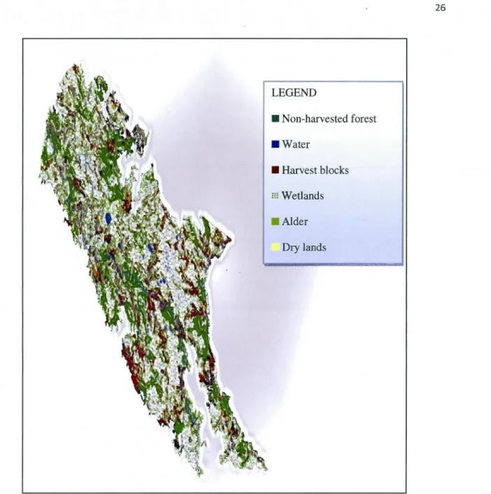
In figure 2.4, harvest blocks are left brown for a better visual appreciation of the management site in its entirety. Non-harvested forest (dark green), planned forest residuals (dark green), water (blue), Aider (light green), wetlands (spotted green) and other coverage types in the eco-forest map (orange). This example is a variable retention logging scenario of 60000 ha with maximum EBM residual forest parameters. It contains 16725 ha of forested area, 774 ha in surface area of water, 38327 ha of wetlands, 417 ha of Aider, 288 ha of dry lands (bright yellow), 13 ha of flood sites, and 15329 ha of Spruce forest stands, to name a few of its characteristics. The image in the upper right corner is a doser look at the bottom left of the logging scenario. The non-harvested forest includes residuals that surround a river, Alder stands, smalllakes, logged areas and the large surface area of wetlands.
LEGEND • Non-harvested forest • Water • Harvest blocks m Wetlands • Aider Dry lands
Figure 2.4 A habitat layer for a 60000 ha variable retention Jogging scenario with maximum forest retention (S6).
*
Non-harvested forest (including retention)- darkgreen; Water-blue; Harvest blocks-brown; Wetlands- spotted green; Alder-light
green; Dry lands-yellow.
2.4 Correlation measurement analyses
A correlation measurement test with JMP® software from SAS (www.jmp.com) was performed for the scenarios in order to compare the influence of each independent variable (1. site size, 2. total residual forests, 3. frequency of peninsulas, insular
blocks and fragments, 4. surface area of peninsulas, insular blocks and fragments, 5. forest harvested, 6. forest non- harvested, 7. forest stand by tree species, 8. forest
stand by density, 9. forest stand by height, 10. km of road network, and 11. surface
area of other land cover types in relation to harvesting effort and habitat quality
index).
Ranking of measurements were based on the Cohen model where 0.5 is large, 0.3 is moderate, and 0.1 is small (Cohen, 1988). The usual interpretation of this statement is
that anything greater than 0.5 is large, 0.5-0.3 is moderate, 0.3-0.1 is small, and
3.1 EBM forest retention scenarios
The forest retention model we created successfully emulated spatial configuration and shape complexity of forest retention found in natural landscapes post fire. However, set parameters were not attained. This could be due to a number of factors including pre-existing forest conditions and geographical influences such as wetlands, water bodies, pre-harvested zones, and other non timber-productive forested areas encountered in a site during simulation. In hindsight, parameters within the model itself can be adjusted and numerous simulations can run until desired targets are met.
Whether our target parameters were greater, lesser or equal than parameters obtained is shown in table 3.1 for the various retention types studied. Results show that forest retention frequency and amount were more variable than initially expected. Two opposing arguments arise: (1) the greater variability found in our sites reflect the non-deterministic characteristic of natural disturbances and the realistic forest availability found in a forest management unit. Or, (2) residual forest models should be more deterministic in order to attain set parameters even if it influences shape complexity and spatial configuration. We chose to keep our simulations stochastic even if site sizes and retention proportions were slightly skewed. At the end of the day, the goal is to achieve better spatial management for ecosystem function and resilience and not to solely emulate a specifie configuration or exact parameter.
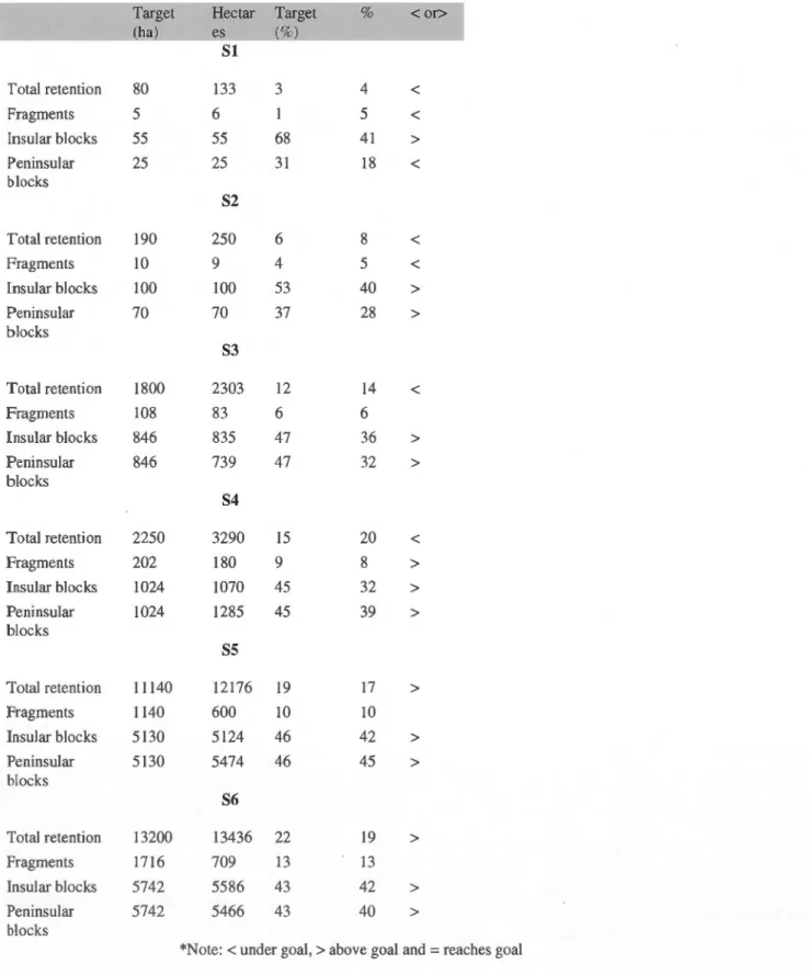
Table 3.1 Comparison of results of residual forest proportion in ha and percentage to our initial target parameters across scenarios.
Target Hectar Target % <or>
ha es %) Sl Total retention 80 133 3 4 < Fragments 5 6 1 5 < Insular blocks 55 55 68 41 > Peninsular 25 25 31 18 < blacks S2 Total retention 190 250 6 8 < Fragments 10 9 4 5 <
Insular blocks lOO 100 53 40 >
Peninsular 70 70 37 28 > blocks S3 Total retention 1800 2303 12 14 < Fragments 108 83 6 6 Insu1ar blocks 846 835 47 36 > Peninsular 846 739 47 32 > blocks S4
Total retention 2250 3290 15 20 <
Fragments 202 180 9 8 > Insular blocks 1024 1070 45 32 > Peninsular 1024 1285 45 39 > blocks
ss
Total retention 11140 12176 19 17 > Fragments 1140 600 10 10 Insular blocks 5130 5124 46 42 > Peninsular 5130 5474 46 45 > blocks S6Total retention 13200 13436 22 19 >
Fragments 1716 709 13 13
lnsular blocks 5742 5586 43 42 >
Peninsular 5742 5466 43 40 >
blocks
3.2 Harvesting effort for variable retention logging scenarios based on EBM indicators
Table 3.2 shows the mean harvesting effort across scenarios that were calculated in ArcGIS. Site size refers to the average size of the logging site in ha, SA harvested refers to the surface area of timber-productive forest harvested in ha, m3*ha refers to
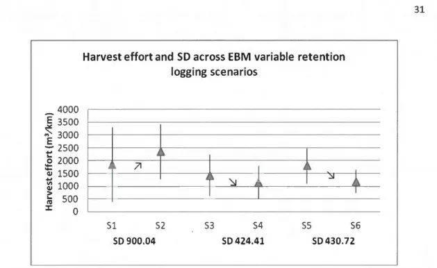
total volume of timber-productive forest harvested in cubic meters (m3), km represents the average length of the road network of each site and Harvesting effort calculate for each scenario. Table 3.2 also shows the standard deviation between variables per site size (3000 ha, 15000 ha, 60000 ha). In addition, in the maximum scenarios for logging sites of 15000 ha and 60000 ha, less timber-productive forest was harvested. In 15000 ha logging sites, a standard deviation of 938.49 ha of SA harvested was found between scenarios with minimum and maximum retention. In sites of 60000 ha a standard deviation of 3548.51 ha of SA harvested was found between scenarios with minimum and maximum retention. Figure3.1 illustrates how these results compare to harvesting effort across scenarios.
Table 3.2 Mean and SD across EBM scenarios
r
Scenario Site size SA Harvested m3*ha KM Harvest Effort1 SI 3099 686 56438 32 1697 S2 3120 949 73435 33 2216 SD 29.54 370.57 32181.62 5.32 366.98 S3 16361 3296 204862 147 1393 S4 16211 2676 151905 142 1083 SD 667.58 938.49 66647.01 23.32 219.20 S5 69245 12818 920795 547 1685 S6 69840 9479 688727 534 1287 SD 2652.66 3548.51 257935.3 67.08 281.42
4000 E 3500
~
3000 : 25002
2000 ~ 1500 ~ 1000 > )ii 500 ::t: 0Harvest effort and SD across EBM variable retention logging scenarios A~
~
~~ .71 51 52 53 SD 900.04 ~t
54 SD 424.41 ~· 55~
t
56 SD 430.72Figure 3.1 Average harvesting effort ac ross scenarios. Li nes represent maximum and minimum effort for each. Triangles represent average for each scenario. And SD
represents the standard deviation within scenario groups.
The figure 3.1 shows the variability of harvest effort between scenarios. Scenario S2 of 3000 ha show a higher harvest effort. A high harvest effort is related to a lower cost estimate. In, all other maximum retention scenarios, where average SA timber-productive forest harvested is lower and forest retention is higher, lower harvest efforts are found as predicted. The length of road networks (total km) did not seem to be significant as SD between sites is small. However, in order to compare harvesting effort calculations to business as usual scenarios, it is important to note that pre
-existing roads were not incorporated. Thus actual harvest effort for our logging
scenarios could have been lower had our initial simulations in SELES incorporated
pre-existing road networks. Pre-existing road networks were only added post
simulation in ArcGIS, however, too many forest retention patches fell directly on
roads, so they were not included in this analysis. Table 3.3 outlines the average
Table 3.3 Average pre-existing kilometers of road for each scenario Scenario 3000 15000 60000 Km 7 67 323
3.3 Impacts of retention patch types and other forest conditions on harvesting effort
One of the objectives of this project was to evaluate different EBM variable retention Jogging scenarios in order to calculate their harvesting effort to verify that the greater the percentage of residual forests, the higher the cost (Bennett, 2003; Perron, 2003; Y elle et al., 2009). Our results show this to be true, for ail sites except our variable retention Jogging scenarios of 3000 ha with maximum retention. Although S2
scenarios contained maximum retention, they also obtained greater harvesting yields.
This could explain why harvesting effort was higher. In order to test what other site
variables could be impacting harvesting efforts a correlation analysis was executed.
When analyzing the impacts of residual patch type proportion and frequency individually we found that the surface area of insular blocks was the only residual patch type that bad a positive relationship with harvesting effort (Table 3.4). Therefore an increase in the proportion of insular block and harvesting effort signifies lower cost estimates. The forest residual that bad the greatest relationship to harvest
effort was the proportion of fragments. However, the relationship was negative, thus
having the most impact on cost estimation. Both the amount of fragments and
peninsulas bad negative relationships with harvesting effort. However, fragments bad
the highest correlation measurement (moderate as opposed to low-moderate with
harvesting effort). No correlations were found between any of the residual forest
patch frequencies and harvesting effort. Other forest conditions were also influential
on harvesting effort. The largest relationships found were between harvest effort and
forest stands 17 to 22 rn high and wetlands. As weil as moderate relationships
Spruce, and mature forests. This could be due to the fact that forest stands with such characteristics have higher levels of volume, and therefore decrease effort.
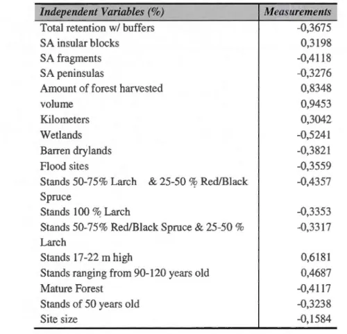
Table 3.4 Correlation measurements (Cohen) for harvest effort across scenarios Independent Variables (%)
Total retention w/ buffers SA insular blocks
SA fragments
SA peninsulas
A mount of forest harvested
volume
Kilometers
Wetlands
Barren drylands Flood sites
Stands 50-75% Larch & 25-50% Red/Black Spruce
Stands 100 o/cz Larch
Stands 50-75% Red/Black Spruce & 25-50%
Larch
Stands 17-22 rn high
Stands ranging from 90-120 years old
Mature Forest
Stands of 50 years old
Site size Measurements -0,3675 0,3198 -0,4118 -0,3276 0,8348 0,9453 0,3042 -0,5241 -0,3821 -0,3559 -0,4357 -0,3353 -0,3317 0,6181 0,4687 -0,4117 -0,3238 -0,1584
3.4 Impacts of retention patch types and other forest conditions on habitat quality index for moose (Alces alces), marten (Martes americana), and hare (Lepus americanus)
The results of the HQI calculations with extension 3.0 in ArcGIS shown below in figure 3.2 indicate that all EBM variable retention logging scenarios offered mostly weak habitats for moose. Under the Courtois (1993) model for moose, habitats with a weak attraction value are black spruce stands, open areas as a result of harvests or burns that occurred less than 10 years prior, and protection covers of 25 to 60 %. It is important to reiterate that these are conditions post logging. On average there was 0
to 2 % optimal habitat, 4 to 10 % medium habitat and 86 to 92 % weak habitats across our scenarios post cuts for this species.
100% 90% 80% 70% 60% 50% 40% 30% 20% 10% 0% 51 52 53 54 55 56 • % strong 0 0 0 0 0 0 • % medium 7 7 10 8.5 4 4.5 • %weak 92 92 86 87 88.5 90.5 • % null 3 3 5.5 5.5 3.5 4.5
Figure 3.2 Proportion of habitat quality index across scenarios for moose
(S l,S2 :3000 ha; S3, S4: 15000 ha; S5, S6: 60000 ha).
The HQI results for marten are shown in figure 3.3. Post cuts, there was 0.5 to 4% optimal habitat, 7 to 11.5 medium habitat, 10 to 24.5 weak habitat with null habitat
representing the majority of forest available. This could be explained to the low
attraction value of Black/ Red spruce dominant stands with low coverage densities of
40 % or less (Larue, 1992). Figure 3.4 shows as expected, mostly null habitat quality
for hare. Optimal habitat was found to be lowest for hare at 0 to 0.5 %, even though this species has a smaller home range. On average, 15.5 to 29 % medium habitat
quality was found. Across scenarios an average of 7 to 11.5 % weak habitat was
found. Under the Guay (1994) model for hare, habitats with a weak attraction value for this species are residual forests that are surrounded by eut blocks, areas in the process of regeneration, or areas that have been harvested 10 years prior or less. This ex plains the higher percentages of null habitat.
100% 90% 80% 70% 60% 50% 40% 30% 20% 10% 0% 51 52 53 54 55 56 • strong habitat 2.5 2.5 0.5 1 4 1.5 • medium habitat 8.5 8 9 7 11.5 17.5 • weak habitat 24.5 14.5 19 23.5 17 10 • nu li habitat 67.5 82 71 67 72.5 69
Figure 3.3 Proportion of habitat quality across scenarios for marten CS 1, S2: 3000 ha;
S3, S4: 15 000 ha; S5, S6: 60 000 ha). 100% 90% 80% 70% 60% 50% 40% 30% 20% 10% 0% 51 52 53 54 55 56 • strong habitat 0 0 0.5 0.03 0.05 0.05 • medium habitat 23 15.5 20.5 29 18.5 20 • weak habitat 8.5 7 7 8.5 10.5 11.5 • nu li habitat 67.5 75 70.5 72 72.5 69
Figure 3.4 Proportion of habitat quality across scenarios for hare CS 1, S2: 3000 ha; S3, S4: 15000 ha; S5, S6: 60000 ha).
When comparing our HQI across scenarios for each species to table 3.2, we find that the habitat quality index does not increase with total retention amounts (TR). If it did, we would find that scenarios S2, S4, and S6 (scenarios with maximum forest retention) would be the most favourable. However, for moose, S 1 and S2 fared equally, and S3 fared better than S4. Better habitat quality existed in scenarios S 1, S3 and S5 for marten, while hare habitat was best in scenarios S 1, S4 and S6. In order, to identify the impacts of retention patch types and other forest conditions, correlation measurement analyses were executed for each species (Table 3.5 to 3.7).
Table 3.5 Correlation measurement test for moose habitat quality (Alces alces)
Variables(%) Null Weak Medium High
Site size 0,5359 0,4241
Tot. retention w/ buffers 0,5456 0,3976
N. of insular blocks 0,5433 0,4424
Area of insular blocks 0,5633 0,4325
N. of fragments 0,5163 N. of Peninsulas 0,5386 0,4443 Area of peninsulas 0,5014 Harvested -0,7004 V o. * ha (m3) -0,6353 Km ofroad -0,674
Non harvested 0,4023
Area of fragments 0,4792
Looking at the weak habitat availability in our variable retention Jogging sites, the
low HQI had significant relationships with the surface area harvested, volume
harvested and kilometers of roads, which would all be expected (Table 3.5). As for retention patch types, the frequency of peninsulas and insular blocks had stronger relationships to HQI than their proportions. However, the proportion of insular blocks
was also important. The medium and high habitat quality forest areas were related to