This is an author-deposited version published in :
http://oatao.univ-toulouse.fr/
Eprints ID : 5661
To link to this article : DOI: 10.1109/TSP.2012.2186132
URL : http://dx.doi.org/10.1109/TSP.2012.2186132
O
pen
A
rchive
T
OULOUSE
A
rchive
O
uverte (
OATAO
)
OATAO is an open access repository that collects the work of Toulouse researchers and
makes it freely available over the web where possible.
To cite this version :
Parreira, Wemerson D. and Bermudez, José Carlos M.
and
Richard, Cédric and Tourneret, Jean-Yves
Stochastic Behavior
Analysis of the Gaussian Kernel Least
-Mean-Square Algorithm
.
(2012) IEEE Transactions on Signal Processing, vol. 60 (n° 5). pp.
2208-2222. ISSN 1053-587X
Any correspondence concerning this service should be sent to the repository
administrator:
[email protected]
Stochastic Behavior Analysis of the Gaussian Kernel
Least-Mean-Square Algorithm
Wemerson D. Parreira, José Carlos M. Bermudez, Senior Member, IEEE, Cédric Richard, Senior Member, IEEE,
and Jean-Yves Tourneret, Senior Member, IEEE
Abstract—The kernel least-mean-square (KLMS) algorithm
is a popular algorithm in nonlinear adaptive filtering due to its simplicity and robustness. In kernel adaptive filters, the statistics of the input to the linear filter depends on the parameters of the kernel employed. Moreover, practical implementations require a finite nonlinearity model order. A Gaussian KLMS has two design parameters, the step size and the Gaussian kernel bandwidth. Thus, its design requires analytical models for the algorithm behavior as a function of these two parameters. This paper studies the steady-state behavior and the transient behavior of the Gaussian KLMS algorithm for Gaussian inputs and a finite order nonlinearity model. In particular, we derive recursive expressions for the mean-weight-error vector and the mean-square-error. The model predictions show excellent agreement with Monte Carlo simulations in transient and steady state. This allows the explicit analytical determination of stability limits, and gives opportunity to choose the algorithm parameters a priori in order to achieve prescribed convergence speed and quality of the estimate. Design examples are presented which validate the theoretical analysis and illustrates its application.
Index Terms—Adaptive filtering, kernel least-mean-square
(KLMS), convergence analysis, nonlinear system, reproducing kernel.
I. INTRODUCTION
M
ANY practical applications (e.g., in communications and bioengineering) require nonlinear signal pro-cessing. Nonlinear systems can be characterized by represen-tations ranging from higher-order statistics to series expansion methods [1]. Nonlinear system identification methods based on reproducing kernel Hilbert spaces (RKHS) have gained popularity over the last decades [2], [3]. More recently, kernel adaptive filtering has been recognized as an appealing solution to the nonlinear adaptive filtering problem, as working in RKHS allows the use of linear structures to solve nonlinear estimation problems. See [4] for an overview. The block diagram of a kernel-based adaptive system identification problem is shownW. D. Parreira J. C. M. Bermudezis with the Federal University of Santa Catarina, Florianópolis, SC, Brazil (e-mail: [email protected]; [email protected]).
C. Richard is the Université de Nice Sophia-Antipolis, Institut Universitaire de France, France (e-mail: [email protected]).
J.-Y. Tourneret is with the Université de Toulouse, CNRS, France (e-mail: [email protected]).
Digital Object Identifier 10.1109/TSP.2012.2186132
in Fig. 1. Here, is a compact subspace of
is a reproducing kernel, is the induced RKHS with its inner product and is a zero-mean additive noise uncorrelated with any other signal. The representer theorem [2] states that the function which minimizes the squared
estimation error , given input
vectors and desired outputs , can be written as the
kernel expansion . This reduces
the problem to determining that minimizes , where is the Gram matrix with th entry , and . Since the order of the model is equal to the number of available data , this approach cannot be considered for online applications. To overcome this barrier, one can focus on finite-order models
(1)
where form a subset of
cor-responding to the time indexes of the input vectors chosen to build the th-order model (1). The kernel func-tions form the dictionary. In [4], the authors present an overview of the existing techniques to select the kernel func-tions in (1), an example of which is the approximate linear de-pendence (ALD) criterion [5]. It consists of including a kernel function in the dictionary if it satisfies
(2)
where is a parameter determining model sparsity level. To control the model order with reduced computational complexity, the coherence-based sparsification rule has also been considered [6], [7]. According to this rule, kernel is inserted into the dictionary if
(3) with a parameter determining the dictionary coherence. It was shown in [7] that the dictionary dimension determined under rule (3) is finite. For the rest of the paper, we shall assume that the dictionary size is known, fixed and finite.
It is well known that a nonlinear adaptive filtering problem with input signal in can be solved using a linear adaptive filter [4]. The linear adaptive filter input is a nonlinear mapping of to an Hilbert space possessing a reproducing kernel. The theory outlined above shows that the order of the linear adap-tive filter can be finite if a proper input sparsification rule is em-ployed, even if the dimensionality of the transformed input in
Fig. 1. Kernel-based adaptive system identification.
is infinite as in the case of Gaussian kernel. Algorithms de-veloped using these ideas include the kernel least-mean-square (KLMS) algorithm [8], [9], the kernel recursive-least-square (KRLS) algorithm [5], the kernel-based normalized least-mean-square (KNLMS) algorithm and the affine projection (KAPA) algorithm [6], [10], [7]. See also the monograph [4]. In addition to the choice of the usual linear adaptive filter parameters, de-signing kernel adaptive filters requires the choice of the kernel and its parameters. Moreover, using the finite order model in (1) implies that the adaptive algorithm behavior cannot be studied as the behavior of the algorithm presented in [4, (2.17)], which is a regular LMS algorithm operating in the RKHS. Choosing the algorithm and nonlinearity model parameters to achieve a prescribed performance is still an open issue, and requires an ex-tensive analysis of the algorithm stochastic behavior. Our work brings a new contribution to the discussion about kernel-based adaptive filtering by providing the first convergence analysis of the KLMS algorithm with Gaussian kernel.
The paper is structured as follows. In Section II, we derive recursive expressions for the mean weight error vector and the mean-square error (MSE) for Gaussian inputs. In Section III, we define analytical models for the transient behavior of the first and second-order moments of the adaptive weights. Section IV studies the algorithm convergence properties. Sta-bility conditions and a steady-state behavior model are derived which allow the algorithm design for prescribed convergence speed and quality of estimate. In Section V, we use the analysis results to establish design guidelines. Section VI presents design examples which validate the theoretical analysis and illustrate its application. The model predictions show excellent agreement with Monte Carlo simulations both in transient and steady state.
II. MEANSQUAREERRORANALYSIS
Consider the nonlinear system identification problem shown in Fig. 1, and the finite-order model (1) based on the Gaussian kernel
(4)
where is the kernel bandwidth. The environment is assumed stationary, meaning that is stationary for sta-tionary. This assumption is satisfied by several nonlinear systems used to model practical situations, such as memo-ryless, Wiener and Hammerstein systems. System inputs are zero-mean, independent, and identically distributed Gaussian
vectors so that
for . The components of the input vector can, however, be correlated. Let denote their autocorrelation matrix.
For a dictionary of size , let be the vector of kernels at time ,1that is
(5) where is the th element of the dictionary, with
for . Here we consider that the vectors may change at each iteration following some dic-tionary updating schedule. The only limitation imposed in the
following analysis is that for so
that the dictionary vectors which are arguments of different en-tries of are statistically independent. To keep the notation simple, however, we will not show explicitly the dependence of
on and represent as for all .
From Fig. 1 and model (1), the estimated system output is (6)
with . The corresponding
estima-tion error is defined as
(7) Squaring both sides of (7) and taking the expected value leads to the MSE
(8)
where is the correlation matrix
of the kernelized input, and is the cross-correlation vector between and . It is shown in Appendix A that is positive definite. Thus, the optimum weight vector is given by
(9) and the corresponding minimum MSE is
(10) These are the well-known expressions of the Wiener solution and minimum MSE, where the input signal vector has been replaced by the kernelized input vector. Determining the op-timum requires the determination of the covariance matrix
1If the dictionary size is adapted online, assume that is sufficiently large
, given the statistical properties of and the reproducing kernel.
Before closing this section, let us evaluate the correlation ma-trix . Its entries are given by
(11) with . Note that remains time-invariant even if the dictionary is updated at each iteration, as is stationary and and are statistically independent for .
Let us introduce the following notations
(12) where is the norm and
(13) and
(14)
where is the identity matrix and is the null matrix. From [11, p. 100], we know that the moment generating function of a quadratic form , where is a zero-mean Gaussian vector with covariance matrix , is given by
(15) Making in (15), we find that the th element of is given by
(16) with . The main diagonal entries are all equal to and the off-diagonal entries are all equal to
because and are i.i.d. In (16), is the
correlation matrix of vector is the identity ma-trix, and denotes the determinant of a matrix. Finally, note that matrix is block-diagonal with along its diag-onal.
III. GAUSSIANKLMS ALGORITHM: TRANSIENTBEHAVIOR ANALYSIS
The KLMS weight-update equation for the system presented in Fig. 1 is [4]
(17) Defining the weight-error vector leads to the weight-error vector update equation
(18)
From (6) and (7), and the definition of , the error equation is given by
(19) and the optimal estimation error is
(20) Substituting (19) into (18) yields
(21) A. Simplifying Statistical Assumptions
Simplifying assumptions are required in order to make the study of the stochastic behavior of mathematically fea-sible. The statistical assumptions required in different parts of the analysis are the following:
A1: is statistically independent of . This assumption is justified in detail in [12] and has been successfully employed in several adaptive filter analyses. It is called here for further reference “modi-fied independence assumption” (MIA). This assump-tion has been shown in [12] to be less restrictive than the classical independence assumption [13].
A2: The finite-order model provides a close enough
approximation to the infinite-order model with min-imum MSE, so that .
A3: and are uncorrelated. This assumption is also supported by the arguments sup-porting the MIA (A1) [12].
B. Mean Weight Behavior
Taking the expected value of both sides of (21) and using the MIA (A1) yields
(22) which is the LMS mean weight behavior for an input vector
.
C. Mean-Square Error
Using (19) and the MIA (A1), the second-order moments of the weights are related to the MSE through [13]
(23) where is the autocorrelation matrix of and the minimum MSE. The study of the MSE behavior (23) requires a model for . This model is highly affected by the transformation imposed on the input signal by the kernel. An analytical model for the behavior of is derived in the next subsection.
D. Second-Order Moment Behavior
Using (20) and (21), the weight-error vector update becomes
Post-multiplying (24) by its transpose, and taking the expected value, leads to
(25) Using the MIA (A1), the first two expected values are given by
(26) Using assumptions A2 and A3 the third expected value is given by
(27) The fourth and the sixth expected values can be approximated using the MIA (A1), that is,
(28) since by the orthogonality principle [13]. Evaluation of the fifth and seventh expected values requires further simplifications for mathematical tractability. A reason-able approximation that preserves the effect of up to its second-order moments is to assume that and are uncorrelated2. Under both this approximation
and MIA (A1),
(29) where the equality to zero is due to the orthogonality principle.
Using (26)–(29) in (25) yields
(30a) with
(30b)
2Using this approximation we are basically neglecting the fluctuations of
about its mean .
Evaluation of expectation (30b) is an important step in the analysis. In the classical LMS analysis [14], the input signal is assumed zero-mean Gaussian. Then the expectation in (30b) can be approximated using the moment factoring theorem for Gaussian variates. In the present analysis, as is a non-linear transformation of a quadratic function of the Gaussian input vector , it is neither zero-mean nor Gaussian.
Using the MIA (A1) to determine the th element of in (30b) yields
(31) where . Each of the moments in (31) can be determined using (15). Depending on and , we have five different moments to evaluate.
with . Denoting , yields (32) with . Denoting , yields (33) where (34) with . Denoting , yields (35) with . Denoting , yields (36) where (37) with . Denoting (38)
where
(39)
Using these moments, the elements of are finally given by
(40)
and, for
(41)
which completes the evaluation of in (30b). Substituting this result into (30a) yields the following recursive expressions for the entries of the autocorrelation matrix :
(42) and, for
(43)
where and with , as defined
in (16).
E. Some Useful Inequalities
Before concluding this section, let us derive inequalities re-lating the fourth-order moments and the entries of the covari-ance matrix . For real random variables and , remember that Hölder’s inequality says [15]
(44)
where and are in with . As shown
hereafter, this inequality yields
(45) Inequality is obtained by using (44) with
, and . In order to prove inequality , we first need to observe that Hölder’s inequality yields3
(46) The result directly follows from (46) for and . The inequality can be proved using (44) with
and
where the equality is due to stationarity of . Now,
for and
, (44) yields
where the equality is again due to stationarity of . This last relation proves inequality and completes the proof of (45).
Finally, let us state an inequality involving the main diagonal entry of the covariance matrix . By virtue of Cheby-shev’s sum inequality, we have
(47)
In the next section, we shall use the recursive expressions (42) and (43) of the autocorrelation matrix , and (45) and (47) to study the steady-state behavior of the Gaussian KLMS algorithm.
IV. GAUSSIANKLMS ALGORITHM: CONVERGENCEANALYSIS We now determine convergence conditions for the Gaussian KLMS algorithm using the analytical model derived in Section III. Let be the lexicographic representation of , i.e., the matrix is stacked column-wise into a single vector . Consider the family of
matrices , whose elements are given by (48)–(49), shown at the bottom of the page. Finally, we define the matrix as follows:
(50) with the lexicographic representation of . Using these definitions, it can be shown that the lexicographic representation of the recursion (30a) can be written as
(51) where is the lexicographic representation of . We shall use this expression to derive stability conditions for the Gaussian KLMS algorithm. But before closing this subsection, let us remark that matrix is symmetric. This can be shown
from (48)–(49), using , and
observing that . This implies that can be diagonalized by a unitary transformation, and all its eigenvalues are real-valued.
A. Convergence Conditions
A necessary and sufficient condition for convergence of in (51) is that all the eigenvalues of lie inside the open interval
([16], Section 5.9). Thus, the stability limit for can be numerically determined for given values of and . In the following we derive a set of analytical sufficient conditions that can also be used for design purposes.
It is well known that all the eigenvalues of lie inside the union of Gerschgorin disks [17]. Each of these disks is centered at a diagonal element of and has a radius given by the sum of
the absolute values of the remaining elements of the same row. A sufficient condition for stability of (51) is thus given by
(52)
Equations (48)–(50) show that the rows of have only two distinct forms, in the sense that each row of has the same entries as one of these two distinct rows, up to a permutation. This implies that only two distinct Gerschgorin disks can be defined. Also, all the entries of are positive except possibly
for and . See
Appendix B for proof. Expression (52) thus leads to only two inequalities, defined as follows for
(53a)
(53b) The study of the limiting values of that satisfy both (53a) and (53b) yields bounds on the maximum step size. The intersection of these bounds yields the sufficient stability limits. In what fol-lows, we present the analysis for . The results for and are presented in Appendix C.
To determine the bounds imposed by (53a), we write it for as
(54) Thus, the following two conditions must be satisfied
(55a)
(55b)
otherwise,
(48)
TABLE I
CONDITIONS ON DERIVEDFROM(55B)
Condition (55a) yields (56), shown at the bottom of the page, because the numerator and denominator of are positive. On the other hand, (55b) leads us to a condition of the form
with
(57)
(58) Hereafter, we shall denote by the resulting bound on . Then, solving (55b) yields the four possible cases shown in Table I, depending on the signs of and . In case (ii), note that there exists no that satisfies (55b) when and . This situation arises because condition (53a) is a suffi-cient condition imposing that the Gerschgorin disks defined by (52) are completely inside the unit circle in the z-plane. This condition is obviously not necessary for having all the eigen-values of inside the unit circle. The lower bound in case (iv) of Table I is also due to this excessive restriction, as the algo-rithm is certainly stable for . It is kept here for complete-ness, but it should be disregarded in practice.
Combining the possible solutions of (55a) and (55b) and dis-regarding lower bounds yields the following stability bounds for
for case (i) in Table I
for cases (ii) and in Table I (59) If case (iii) happens, which should be tested right away, the sta-bility conditions should be determined numerically through the eigenvalues of .
Having determined limits for (53a) such that , and as-suming that case (iii) in Table I did not happen, we proceed to determine the extra restrictions imposed on by (53b). First, we multiply (53b) by and divide by , rewriting it as
(60)
TABLE II
CONDITIONS ON DERIVEDFROM(62B)
Now, given that (54) has already been satisfied, we replace the left-hand side (LHS) of (60) with the right-hand side (RHS) of (54). After rearranging the terms, we have the new condition
(61) which leads to the following two conditions:
(62a)
(62b) On the one hand, (62a) yields two different conditions defined by if if (63) where (64) On the other hand, (62b) leads us to a condition of the form , where has already been defined in (57) and
(65) Solving (62b) thus leaves four possible cases to consider, shown in Table II, where .
Combing the possible solutions of (62a) and (62b), and again disregarding lower bounds, yields the following stability bounds on [see (66) at the bottom of the page].
Finally, except for cases (iii) in Table I and (vii) in Table II, which should be tested right away, the sufficient stability con-ditions will be given by the intersection of (59) and (66). These conditions can be slightly simplified by observing that , as can be easily proved using (45).
In the next section, we shall derive the expression of the weight-error correlation matrix in steady state. This will allow us to calculate the MSE and the excess MSE.
B. Steady-State Behavior
The closed-form solution of (51) can be written as [16] (67) where denotes the vector in steady state, and is given by
(68) Assuming convergence, we define the time for convergence as the number of iterations required for (67) to reach
(69) where is a design parameter to be chosen by the user.
At this point, it is important to note that is unique if the system under consideration is stable. Indeed, the matrix
has only nonzero eigenvalues because it satisfies conditions (53a)–(53b), and can thus be inverted. Let be the matrix whose lexicographic representation is . It is also unique and satisfies the following expression derived from (30a) for
:
(70) In (70), denotes the matrix in steady state. It is interesting to note that (68) is the lexicographic counterpart of (70), as (51) is the lexicographic representation of (30a).
From (23), the steady-state MSE is given by
(71) where is the steady-state excess MSE, de-noted by . To evaluate these quantities, we shall now compute the entries of . In order to achieve this, we first justify that is a matrix with the same structural proper-ties as , namely, all its main diagonal entries are equal to each other, having a value denoted by , and all its off-diag-onal entries are also equal to each other, having a value denoted by . Then, we determine and so that is the solution to (70), which we know is unique. It is straightforward to see that the LHS of (70) is also a matrix with the same struc-tural properties as , as it is equal to .
One way for to have the proposed structure would
be that and all have the
same structure. It is straightforward to show that matrices and have this structure if, and only if, has that structure. If this is the case, a direct con-sequence, through (70), would be that also has this structure. Using and , respectively, for the main-di-agonal and off-dimain-di-agonal entries of in (40) and (41) yields, for [see (72) at the bottom of the page]. For . Writing, for ease of notation, and
for all , and solving (70) for and yields (73)-(74), shown at the bottom of the page, with and defined in (16).
It can be verified that using (72)–(74) in the LHS of (70) yields the correct RHS. Also, we know that this solution is unique since can be inverted. Then, going back to (71), we obtain the following desired result
(75) Based on the results presented in the previous sections, we shall now propose design guidelines to set the parameters of
If for case in Table II
for cases and in Table II
If for case in Table II
for cases and in Table II (66)
(72)
(73)
the Gaussian KLMS algorithm in order to achieve a prescribed performance.
V. DESIGNGUIDELINES
The analysis results are now used to establish design guide-lines. Without limiting generality, the coherence-based sparsifi-cation rule (3) is considered hereafter to design the dictionaries. It is however implicit that any other existing technique to se-lect the kernel functions could be used. These de-sign guidelines assume the availability of multiple realizations of the sequences and .
Suppose a design goal is to obtain an MSE which is less than a specified value . The following procedure could be applied. 1) Set a coherence threshold and define a set of kernel bandwidths to be tested. For the following design exam-ples, a set of values for was chosen as equally spaced points in (0, 1). Then, was chosen to yield reasonable values of for the chosen set of values. The value of is determined for each pair by training the dic-tionary with the input signal until its size stabilizes. The training is repeated several times. A value is de-termined for the th realization. The value of associated with the pair is the average of the dictionary sizes for all realizations, rounded to the nearest integer. This is the value of to be used in the theoretical model. 2) Using the system input , determine the desired output
and estimate and over several runs. In a practical setting should be measured at the unknown system output.
3) From (10), determine the minimum MSE for each set of parameters . If none of the pairs leads to , return to step 1 to choose a new set of parameters and .
4) Determine using rules (59) and (66) for each value of and choose the largest possible value of so that
and (note that is computed
using (75)).
5) Given and determine using (50) and then from (51).
6) Determine from (73)–(74), and then from (75).
7) Choose in criterion (69) and find from simulations using the parameters determined in steps 1 to 8.
Repeat steps 1 to 9 for all kernel parameters in the chosen set and use the one that leads to the smallest .
VI. SIMULATIONRESULTS
This section presents examples to illustrate the proposed de-sign procedure and to verify the theoretical results. The sim-ulation conditions which are common to all examples are de-scribed in Example 1. Only the changes to these conditions are described in the remaining examples.
A. Example 1
Consider the problem studied in [18] and [19], for which
(76)
TABLE III
STABILITYRESULTS FOREXAMPLE1
TABLE IV
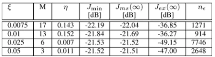
SUMMARY OFSIMULATIONRESULTS FOREXAMPLE1
where the output signal was corrupted by a zero-mean white Gaussian noise with variance . The input sequence is zero-mean i.i.d. Gaussian with standard
devi-ation .
The proposed method was tested with a maximum MSE dB, a coherence level and a set of
kernel bandwidths 4. For each
value of , 500 dictionary dimensions , were determined using 500 realizations of the input process. The length of each realization was 500 samples. Each was de-termined as the minimum dictionary length required to achieve the coherence level . The value was determined as the average of all , rounded to the nearest integer. The values of were calculated from (10) for each pair . To this end, second-order moments and were estimated by averaging over 500 runs.
Before searching for a value of , such that , we have to define . There are two possibilities for defining : 1) use the Gerschgorin disk analysis yielding a value of
denoted as , 2) compute and test the eigenvalues of yielding a value of denoted as . Table III shows that, as expected, the condition imposed by the Gerschgorin disks is more restrictive than that imposed by the eigenvalues of . However, note that choosing from is simpler and usually yields good design results.
Table IV presents the obtained results for the chosen values of . For each pair , the step-size was chosen so that the al-gorithm was stable ( less than ) and dB. The values of and were determined from (75) and was obtained from (69) for . Note that dB in all cases. It clearly appears that is a good design choice, as it satisfies all design conditions after only iterations. Note that the value of chosen is about 1/10 of . This is due to the small value of imposed by the design. This is the same phenomenon that happens when designing the regular LMS algo-rithm for practical specifications in linear estimation problems. For each simulation, the order of the dictionary remained fixed. It was initialized for each realization by generating input
4These values of are samples within a range of values experimentally
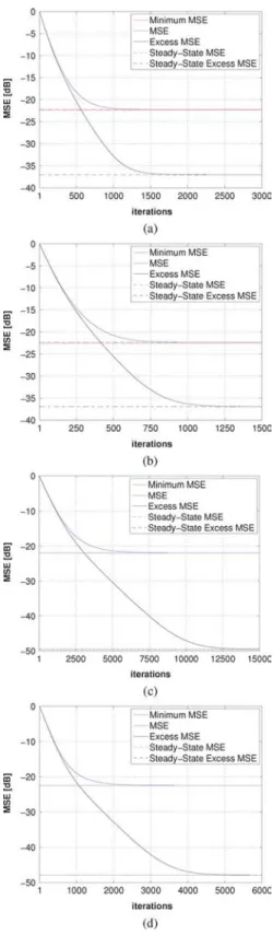
Fig. 2. Theoretical model and Monte Carlo simulation of KLMS for different kernel bandwidths. Ragged curves (blue): simulation results averaged over 500 runs. Continuous curves (red): Theory using (23) and (67). Continuous hori-zontal lines (blue): Steady-state MSE predicted by theory. Dashed horihori-zontal lines (red): Steady-state MSE from simulations. (a) and .
(b) and . (c) and . (d) and
.
vectors in and filling the positions with vectors that sat-isfy the desired coherence level. Thus, the initial dictionary is different for each realization. During each realization, the dic-tionary elements were updated at each iteration so that the least recently added element is replaced with .
Figs. 2 and 3 illustrate the accuracy of the analytical model for the four cases presented in Table IV. Fig. 2 shows an ex-cellent agreement between Monte Carlo simulations, averaged
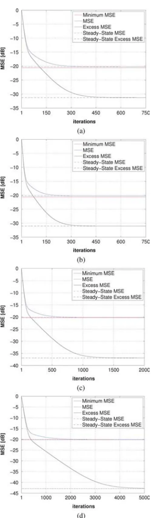
Fig. 3. Steady-State results. Dashed horizontal lines: MSE and Excess MSE averaged over 500 realizations. Continuous horizontal lines (red): Minimum MSE predicted by theory. Continuous decaying lines: Theoretical MSE (blue) and Excess MSE (black). (a) and . (b) and
. (c) and . (d) and .
over 500 runs, and the theoretical predictions made by using (23) and (67). Fig. 3 compares simulated steady-state results (dashed horizontal lines) with theoretical predictions using (68). There is again an excellent agreement between theory and simulations.
TABLE V
STABILITYRESULTS FOREXAMPLE2
TABLE VI
SUMMARY OFSIMULATIONRESULTS FOREXAMPLE2
B. Example 2
As a second design example, consider the nonlinear dynamic system identification problem studied in [20] where the input signal was a sequence of statistically independent vectors
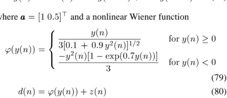
(77) with correlated samples satisfying . The second component of in (77) is an i.i.d. Gaussian noise sequence with variance and is a white Gaussian noise with variance . Consider a linear system with memory defined by
(78) where and a nonlinear Wiener function
(79) (80) where is the output signal, corrupted by a zero-mean white Gaussian noise with variance . The initial con-dition was considered in this example.
The proposed method was tested with a maximum MSE dB, a coherence level and a set of
kernel bandwidths . The other
simulation conditions were similar to the first example. Table V shows the estimated values of obtained with the Gerschgorin disk analysis and from the eigenvalues of . The expression without solution (w.s.) indicates that the intersection of solutions provided by (59) and (66) is empty. In this case, we need to use the limit obtained from the eigenvalues of , i.e.,
.
Table VI presents the obtained results for the chosen values of . For each pair , the step-size was chosen in order to ensure algorithm stability ( less than ) and
dB. The values of and were deter-mined from (75) and was obtained from (69) for . Note that dB in all cases. It clearly appears
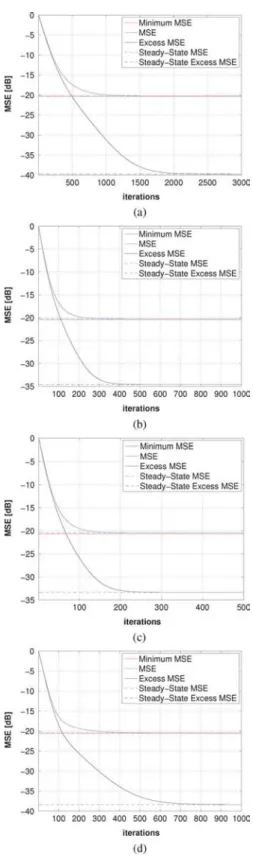
Fig. 4. Theoretical model and Monte Carlo simulation of KLMS for different kernel bandwidths. Ragged curves (blue): simulation results averaged over 500 runs. Continuous curves (red): Theory using (23) and (67). Continuous hori-zontal lines (blue): Steady-state MSE predicted by theory. Dashed horihori-zontal lines (red): Steady-state MSE from simulations. (a) and .
(b) and . (c) and . (d) and
.
that is a good design choice as it satisfies all design conditions after iterations.
Fig. 5. Steady-State results. Dashed horizontal lines: MSE and Excess MSE averaged over 500 realizations. Continuous horizontal lines (red): Minimum MSE predicted by theory. Continuous decaying lines: Theoretical MSE (blue) and Excess MSE (black). (a) and . (b) and .
(c) and . (d) and .
Figs. 4 and 5 illustrate the accuracy of the analytical model for the four cases presented in Table VI. The agreement between theory and simulations is excellent as in the first example.
TABLE VII
STABILITYRESULTS FOREXAMPLE3
TABLE VIII
SUMMARY OFSIMULATIONRESULTS FOREXAMPLE3
C. Example 3
As a third design example, consider the fluid-flow control problem studied in [21] and [22] whose input signal was a se-quence of statistically independent vectors
(81) with correlated samples satisfying , where is a white Gaussian noise sequence with variance and is a white Gaussian so that has variance . Consider a linear system with memory defined by
(82) with and a nonlinear Wiener function
(83)
where the output signal was corrupted by a zero-mean white Gaussian noise with variance .
The design paramenters were set to dB (maximum MSE), (coherence level) and (set of possible kernel band-widths).
Table VII shows the values of obtained by testing the eigenvalues of . Note that the Gerschgorin disk conditions were too strict for all cases making the computation of impossible.
Table VIII presents the obtained results for the chosen values of . For each pair , the step-size was chosen to ensure stability ( less than ) and dB. The values of and were determined from (75) and
was obtained from (69) for . Note that dB in all cases. It clearly appears that
is a good design choice, as it satisfies the de-sign conditions after iterations.
Figs. 6 and 7 illustrate the accuracy of the analytical model for the four cases presented in Table VIII. Again, the results are very promising for this example.
Fig. 6. Theoretical model and Monte Carlo simulation of KLMS for different kernel bandwidths. Ragged curves (blue): simulation results averaged over 500 runs. Continuous curves (red): Theory using (23) and (67). Continuous hori-zontal lines (blue): Steady-state MSE predicted by theory. Dashed horihori-zontal lines (red): Steady-state MSE from simulations. (a) and . (b)
and . (c) and . (d) and .
VII. CONCLUSION
This paper studied the stochastic behavior of the Gaussian KLMS adaptive algorithm for Gaussian inputs and nonlin-earities which preserve the stationarity of their inputs. The study resulted in analytical models that predict the behavior
Fig. 7. Steady-State results. Dashed horizontal lines: MSE and Excess MSE averaged over 500 realizations. Continuous horizontal lines (red): Minimum MSE predicted by theory. Continuous decaying lines: Theoretical MSE (blue) and Excess MSE (black). (a) and . (b) and .
(c) and . (d) and .
of the algorithm as a function of the design parameters. In particular, the new models clarify the joint contribution of the kernel bandwidth and the step-size for the algorithm performance, both during the transient adaptation phase and in steady state. The algorithm convergence was studied and analytical expressions were derived which provide sufficient
stability conditions. Design guidelines were proposed using the theoretical model. These guidelines were applied to different nonlinear system identification problems. Simulation results have illustrated the accuracy of the theoretical models and their usefulness for design purposes. The extension of this analysis to the case of time-varying systems will be the subject of future investigations.
APPENDIXA POSITIVE-DEFINITENESS OF
To prove that is positive definite we prove that all its eigenvalues are positive [17]. Let and
be, respectively, the th eigenvalue and the corresponding eigen-vector of . Hence,
(84) From (16), we can write as
(85)
where and is the identity
matrix. Using (85) in (84) yields
(86) Noting that , with is an eigenvector of we have
(87) which yields
(88) which is positive since ( is real and is the result of a square root in (16)) and .
The remaining eigenvectors are orthogonal to . Thus, for all and thus
(89) which yields
(90) which are also positive since . This concludes the proof.
APPENDIXB
SIGNANALYSIS OFMATRIX ENTRIES
We shall now analyze the sign of the entries of matrix de-fined in (48)–(49). On the one hand, we know that
and are strictly positive. On the other hand,
and can be either positive or negative de-pending on . The analysis of the diagonal entries of needs more attention.
Consider first . This is a second-degree polynomial with respect to the parameter whose minimum value is . Using (45) and (47), we know that .
This implies that for all . Let us focus now on , whose minimum is equal to . Similarly as above, we know that , which
means that for all .
As a conclusion, all the diagonal entries of the matrix are strictly positive, which greatly simplifies the analysis of (52) for stability.
APPENDIXC
STABILITYANALYSIS IN THECASES AND
Let us first derive the condition for stability of the system (51) in the case . The matrix reduces to the entry . This directly implies that the system (51) is stable if
(91) Consider now the case . Expression (52) leads us to the following two inequalities:
(92a)
(92b) We observe that the LHS of (92a) is larger than the LHS of (92b) for all because , as shown by (45). Proceeding the same way as we did for in Section IV-A, we conclude that (51) is stable if the following conditions are satisfied:
(93) where
(94)
REFERENCES
[1] M. Schetzen, The Volterra and Wiener Theory of the Nonlinear
Sys-tems. New York: Wiley, 1980.
[2] G. Kimeldorf and G. Wahba, “Some results on Tchebycheffian spline functions,” J. Math. Anal. Appl., vol. 33, pp. 82–95, 1971.
[3] D. L. Duttweiler and T. Kailath, “An RKHS approach to detection and estimation theory: Some parameter estimation problems (Part V),”
IEEE Trans. Inf. Theory, vol. 19, no. 1, pp. 29–37, 1973.
[4] W. Liu, J. C. Principe, and S. Haykin, Kernel Adaptive Filtering. New York: Wiley, 2010.
[5] Y. Engel, S. Mannor, and R. Meir, “Kernel recursive least squares,”
IEEE Trans. Signal Process., vol. 52, no. 8, pp. 2275–2285, 2004.
[6] P. Honeine, C. Richard, and J. C. M. Bermudez, “On-line nonlinear sparse approximation of functions,” in Proc. IEEE ISIT’07, Nice, France, Jun. 2007, pp. 956–960.
[7] C. Richard, J. C. M. Bermudez, and P. Honeine, “Online prediction of time series data with kernels,” IEEE Trans. Signal Process., vol. 57, no. 3, pp. 1058–1067, Mar. 2009.
[8] W. Liu, P. P. Pokharel, and J. C. Principe, “The kernel least-mean-squares algorithm,” IEEE Trans. Signal Process., vol. 56, no. 2, pp. 543–554, Feb. 2008.
[9] P. Bouboulis and S. Theodoridis, “Extension of Wirtinger’s calculus in reproducing kernel Hilbert spaces and the complex kernel LMS,” IEEE
[10] K. Slavakis and S. Theodoridis, “Sliding window generalized kernel affine projection algorithm using projection mappings,” EURASIP J.
Adv. Signal Process., vol. 2008, 2008.
[11] J. Omura and T. Kailath, “Some Useful Probability Distributions,” Stanford Electron. Lab., Stanford Univ., Stanford, CA, Tech. Rep. 7050-6, 1965.
[12] J. Minkoff, “Comment: On the unnecessary assumption of statistical independence between reference signal and filter weights in feedfor-ward adaptive systems,” IEEE Trans. Signal Process., vol. 49, no. 5, p. 1109, May 2001.
[13] A. H. Sayed, Fundamentals of Adaptive Filtering. Hoboken, NJ: Wiley, 2003.
[14] S. Haykin, Adaptive Filter Theory, 2nd ed. Englewood Cliffs, NJ: Prentice-Hall, 1991.
[15] G. Grimmett and D. Stirzaker, Probability and Random Processes. New York: Oxford Univ. Press, 2001.
[16] D. G. Luenberger, Introduction Dynamic Systems: Theory, Models &
Applications. New York: Wiley, 1979.
[17] G. H. Golub and C. F. V. Loan, Matrix Computations. Baltimore, MD: The Johns Hopkins Univ. Press, 1996.
[18] K. S. Narendra and K. Parthasarathy, “Identification and control of dy-namical systems using neural networks,” IEEE Trans. Neural Netw., vol. 1, no. 1, pp. 3–27, Mar. 1990.
[19] D. P. Mandic, “A generalized normalized gradient descent algorithm,”
IEEE Signal Process. Lett., vol. 2, pp. 115–118, Feb. 2004.
[20] J. Vörös, “Modeling and identification of wiener systems with two-segment nonlinearities,” IEEE Trans. Contr. Syst. Technol., vol. 11, no. 2, pp. 253–257, Mar. 2003.
[21] J.-S. Wang and Y.-L. Hsu, “Dynamic nonlinear system identification using a Wiener-type recurrent network with okid algorithm,” J. Inf. Sci.
Eng., vol. 24, pp. 891–905, 2008.
[22] H. Al-Duwaish, M. N. Karim, and V. Chandrasekar, “Use of multilayer feedforward neural networks in identification and control of wiener model,” in Proc. Contr. Theory Appl., May 1996, vol. 143, no. 3.
Wemerson D. Parreira was born in Uberaba, Brazil, on March 15, 1978. He received the bachelor’s de-gree in mathematics in 2002 and the M.Sc. dede-gree in electrical engineering from the Federal University of Uberlândia in 2005.
He is currently a doctoral student in electrical en-gineering at the Federal University of Santa Catarina, Florianópolis, Brazil. He worked as a professor in the Department of Informatics and Statistics, the Federal University of Santa Catarina (2006–2007). His expe-rience is in mathematical modeling, with emphasis on Electrical Engineering. His current research interests include reproducing ker-nels, nonlinear filtering, adaptive filtering and statistical analysis.
José Carlos M. Bermudez (M’85–SM’02) received the B.E.E. degree from the Federal University of Rio de Janeiro (UFRJ), Rio de Janeiro, Brazil, the M.Sc. degree in electrical engineering from COPPE/UFRJ, and the Ph.D. degree in electrical engineering from Concordia University, Montreal, Canada, in 1978, 1981, and 1985, respectively.
He joined the Department of Electrical En-gineering, Federal University of Santa Catarina (UFSC), Florianópolis, Brazil, in 1985. He is cur-rently a Professor of electrical engineering. In the winter of 1992, he was a Visiting Researcher with the Department of Electrical Engineering, Concordia University. In 1994, he was a Visiting Researcher with the Department of Electrical Engineering and Computer Science, University of California, Irvine (UCI). His research interests have involved analog signal processing using continuous-time and sampled-data systems. His recent re-search interests are in digital signal processing, including linear and nonlinear
adaptive filtering, active noise and vibration control, echo cancellation, image processing, and speech processing.
Prof. Bermudez served as an Associate Editor of the IEEE TRANSACTIONS ON SIGNALPROCESSINGin the area of adaptive filtering from 1994 to 1996 and from 1999 to 2001. He also served as an Associate Editor of the EURASIP Journal
of Advances on Signal Processing from 2006 to 2010. He was a member of
the Signal Processing Theory and Methods Technical Committee of the IEEE Signal Processing Society from 1998 to 2004.
Cédric Richard (S’98–M’01–SM’07) was born on January 24, 1970, in Sarrebourg, France. He received the Dipl.-Ing. and the M.S. degrees in 1994 and the Ph.D. degree in 1998 from the University of Tech-nology of Compiègne (UTC), France, all in electrical and computer engineering.
He joined the Côte d’Azur Observatory, Univer-sity of Nice Sophia-Antipolis, France, in 2009. He is currently a Professor of electrical engineering. From 1999 to 2003, he was an Associate Professor at the University of Technology of Troyes (UTT), France. From 2003 to 2009, he was a Professor at the UTT, and the supervisor of a group consisting of 60 researchers and Ph.D. students. In winter 2009 and au-tumn 2010, he was a Visiting Researcher with the Department of Electrical Engi-neering, Federal University of Santa Catarina (UFSC), Florianòpolis, Brazil. He has been a junior member of the Institut Universitaire de France since October 2010. He is the author of more than 120 papers. His current research interests include statistical signal processing and machine learning.
Dr. Richard was the General Chair of the XXIth Francophone conference GRETSI on Signal and Image Processing that was held in Troyes, France, in 2007, and of the IEEE Statistical Signal Processing Workshop (IEEE SSP’11) that was held in Nice, France, in 2011. Since 2005, he has been a member of the board of the Federative CNRS research group ISIS on Information, Signal, Images, and Vision. He is a member of the GRETSI association board and of the EURASIP society.
Cédric Richard served as an Associate Editor of the IEEE Transactions on Signal Processing from 2006 to 2010, and of Elsevier Signal Processing since 2009. In 2009, he was nominated liaison local officer for EURASIP, and member of the Signal Processing Theory and Methods Technical Committee of the IEEE Signal Processing Society. Paul Honeine and Cédric Richard received Best Paper Award for “Solving the pre-image problem in kernel machines: a direct method” at the 2009 IEEE Workshop on Machine Learning for Signal Processing (IEEE MLSP’09).
Jean-Yves Tourneret (SM’08) received the ing-nieur degree in electrical engineering from Ecole Nationale Suprieure d’Electronique, d’Electrotech-nique, d’Informatique et d’Hydraulique in Toulouse (ENSEEIHT) in 1989 and the Ph.D. degree from the National Polytechnic Institute from Toulouse in 1992.
He is currently a professor with the University of Toulouse, France (ENSEEIHT) and a member of the IRIT laboratory (UMR 5505 of the CNRS). His re-search activities are centered around statistical signal processing with a particular interest to Bayesian and Markov Chain Monte Carlo methods.
Dr. Tourneret has been involved in the organization of several conferences including the European Conference on Signal Processing (EUSIPCO’2002) (as the Program Chair), the international Conference ICASSP’06 (in charge of ple-naries) and the Statistical Signal Processing Workshop (SSP 2012) (for inter-national liaisons). He has been a member of different technical committees including the Signal Processing Theory and Methods (SPTM) committee of the IEEE Signal Processing Society (2001–2007, 2010–present). He has served as an Associate Editor for the IEEE TRANSACTIONS ONSIGNALPROCESSING (2008–2011).