This is an author-deposited version published in :
http://oatao.univ-toulouse.fr/
Eprints ID : 9250
To link to this article : DOI:
10.1109/MELCON.2012.6196464
URL :
http://dx.doi.org/10.1109/MELCON.2012.6196464
O
pen
A
rchive
T
OULOUSE
A
rchive
O
uverte (
OATAO
)
OATAO is an open access repository that collects the work of Toulouse researchers and
makes it freely available over the web where possible.
To cite this version :
Belouda, Malek and Belhadj, Jamel and Sareni, Bruno
and
Roboam, Xavier and Jaafar, Amine
Synthesis of a compact wind
profile using evolutionary algorithms for wind turbine system with
storage.
(2012) In: 16th IEEE Mediterranean Electrotechnical
Conference (MELECON’12), 25-
28 march 2012, Hammamet,
Tunisia.
Any correspondence concerning this service should be sent to the repository
administrator:
staff-oatao@listes.diff.inp-toulouse.fr
Synthesis of a compact wind profile using evolutionary
algorithms for wind turbine system with storage
Malek Belouda and Jamel Belhadj
University of Tunis, DGE-ESSTT University of Tunis El Manar, LSE-ENITTunis, Tunisia Malek.belouda@google.com
Jamel.Belhadj@esstt.rnu.tn
Bruno Sareni, Xavier Roboam and Amine Jaafar
University of Toulouse, LAPLACE UMR CNRS–INP–UPS,ENSEEIHT 2, Rue Ch Camichel 31071 Toulouse – France sareni@laplace.univ-tlse.fr, roboam@laplace.univ-tlse.fr,
jaafar@laplace.univ-tlse.fr
Abstract— In this paper, the authors investigate two methodologies for synthesizing compact wind speed profiles by means of evolutionary algorithms. Such profile can be considered as input parameter in a prospective design process by optimization of a passive wind system with storage. Compact profiles are obtained by aggregating elementary patterns in order to fulfil some target indicators. The main difference between both methods presented in the paper is related to the choice of these indicators. In the first method, they are related to the storage system features while they only depend on wind features in the second.
I. INTRODUCTION
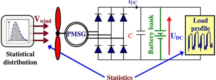
Small renewable energy systems as wind turbine are actually very useful especially for remote areas for electricity production, pumping and water desalination. The design of these systems requires taking account of the wind potential and the load demand. In a prior study [1], a battery sizing methodology has been presented for a 8 kW stand alone passive wind turbine system (see Fig. 1). This method consists in determining the constraints (in terms of power and energy needs) associated with the storage system from temporal Monte-Carlo-based simulations including wind and load profile variations. In this work, the evolution of the wind speed was considered as stochastic while the load profile was deterministically day to day repeated. In order to take account of the wind potential features, multiple dynamics have been integrated in the wind profile, i.e. fast dynamics related to turbulence phenomena as well as slow dynamics related to seasonality represented with a Weibull statistic distribution. Consequently finding the most critical constraints on the storage system requires the system simulation on large time duration in order to include all dynamics (i.e. wind and load profiles dynamics) and all correlations of those variables (e.g. time windows with small wind powers and high load powers and inversely). C UDC IDC Load profile Statistics Vwind B a tt er y b a n k PMSG Statistical distribution
Figure 1. Passive wind system subjected to a wind profile and a load profile
It is shown in [1] that 70 days of system simulation are necessary to obtain an accurate sizing of the battery, allowing the correlation of the load profile with the wind conditions. If this approach can be locally used to optimize the battery sizing when the other components of the passive wind turbine are known, it cannot be applied in a global optimization context [2] requiring a wide number of system simulations. In this case, the computational time would be drastically increased by the repetition of simulations on large time windows. In order to face this issue, we investigate in this paper a methodology for reducing typical wind profile while keeping the wind features in terms of intensity, variability and statistics.
II. SYNTHESISPROCESSOFCOMPACTPROFILES
FORENVIRONEMENTALVARIABLES
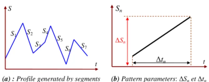
The synthesis process of compact wind profiles is based on the approach developed in [3] for railway driving missions. It consists in generating a fictitious profile of any environmental variable (e.g. temperature, wind speed, solar irradiation…) by fulfilling some constraints related to the variable (typically minimum, maximum and average value, probability distribution function…). These constraints are expressed in terms of target indicators that can be evaluated from a set of real cycles or from a single real cycle of large duration. The fictitious profile is obtained by aggregating elementary segments as shown in Fig. 2. Each segment is characterized by its amplitude ∆Sn (∆Sminref ≤∆Sn≤∆Smaxref) and its duration ∆tn (0≤∆tn≤∆tcompact).
S1 S2 S3 S4 S5 S6 S7 t S t ∆tn ∆Sn Sn
(a) : Profile generated by segments (b) Pattern parameters: ∆Sn et ∆tn
Figure 2. .Principle of the profile generation
A time scaling step is performed after the profile generation in order to fulfil the constraint related to the time duration, i.e. Σ∆tn=∆tcompact. Finding a compact fictitious profile of an environmental variable consists in finding all segment parameters so that the generated profile fulfils all target indicators on the reduced duration ∆tcompact. This results in solving an inverse problem with 2N parameters where N denotes the number of segments in the compact profile. This can be done using evolutionary algorithms [4] and especially with the clearing method [5] well suited to treat this kind of problem with high dimensionality and high multimodality. It should also be noted that the number N of segments can be itself optimized through a self-adaptive procedure [3].
III. APPLICATIONTOCOMPACTPROFILE
SYNTHESISOFWINDSPEED
In this section the synthesis process is applied on an actual wind speed profile of 200 days duration with the aim of generating a compact profile on a reduced duration ∆tcompact. Two different approaches are investigated depending on the choice of the target indicators used for generating the fictitious compact wind speed profile.
A. First method: target indicators are related to storage
system features
The global sizing of the storage system is related to the three following variables: PBATMAX, PBATMIN and ES which respectively denote the maximum and the minimum storage powers in the battery PBAT(t) and the maximum energy quantity imposed to this storage. These variables are extracted from the simulation of a 8 kW passive wind turbine system and used as target indicators in the synthesis process.
Note that the reference value of the storage useful energy ESref is defined as follows:
) ( min ) ( maxEt Et ESref = − (1) where () ( ) [0, ] 0 ref t BAT d t t P t E =
∫
τ τ ∈ ∆Note that E(t) is a saturated integral, with 0 as upper limit so that the battery storage is only sized in discharge mode to avoid oversizing it during wide charge period (huge winds with reduced load). An additional target indicator is considered to take account of statistic features of the reference wind cycle. We use the Cumulative Distribution Function
CDF(Vref) [6]-[8] computed from the corresponding
probability density function (PDFref) related to the reference wind speed behaviour.
0 20 40 60 80 100 120 140 160 180 200 0 10 20 V w in d (m /s ) 0 20 40 60 80 100 120 140 160 180 200 -10 0 10 20 30 P b a t( k W ) 0 20 40 60 80 100 120 140 160 180 200 -30 -20 -10 0 time(days) E (k W h )
Figure 3. Actual ‘reference’ wind speed profile, storage power and energy.
PDFref is evaluated on 20 equally spaced intervals between 0 and the maximum wind speed value Vrefmax. Finally, the global error ε to be minimized in the synthesis profile process can be expressed as:
stat ref ref ref BAT ref BAT BAT ref BAT ref BAT BAT ES ES ES P P P P P P ε ε + − + − + − = 2 2 MIN MIN MIN 2 MAX MAX MAX (2)
where the statistic error εstat denotes the mean squared error between both CDFs relative to reference and generated wind speed profiles:
∑
= − × = 20 1 2 ) ( ) ( ) ( 20 1 k ref ref stat k CDF k CDF k CDF ε (3)All ‘ref’ indexed variables are based on the reference wind profile of Figure 3. The inverse problem has been solved with the clearing algorithm [5] using a population size of 100 individuals and a number of generations of 500 000. Multiple optimization runs were performed with different compaction time ∆tcompact . In particular, the minimum compaction time (i.e. min ∆tcompact) was determined using dichotomous search in order to ensure a global error ε less than 10-2. Table I shows the values of the global error ε versus the compaction time. It can be seen that the lowest value for ∆tcompact ensuring the fulfillment of the target indicators with sufficient accuracy is about 10 days. We give in Fig. 4 the characteristics of the generated wind profile obtained from the aggregation of 109 elementary segments fulfilling all target indicators. It can be seen from this figure that the CDF of this compact wind profile closely coincides with that of the reference wind profile.
TABLE I. INFLUENCEOF∆tcompact.ONTHEGLOBALERRORε
∆tcompact (days) 40 20 10 5 Global error ε ≈ 8.10-3 ≈ 9.10-3 ≈ 9.10-3 ≈ 7.10-2
TABLE II. TARGETINDICATORSOFTHEGENERATEDWIND SPEEDPROFILE. Reference profile Compact profile Error (%) PBATMAX (kW) 30 30 0 PBATMIN (kW) −5.88 −5.82 0.1 ES (kWh) 32.36 32.4 0.12 0 5 10 0 10 20 30 time(days) V w in d (m /s ) 0 5 10 15 20 25 0 0.2 0.4 0.6 0.8 1 Vwind(m/s) C D F reference CDF Generated CDF
Figure 4. Generated wind speed with corresponding CDF.
Table II compares the values of the target indicators related to the battery sizing for the reference and the fictitious profile generated with the clearing algorithm. A good agreement between those values indicates that the compact wind profile will lead to the same battery sizing as the reference wind profile on larger duration.
B. Second method: target indicators only related to the
wind features
In this second approach target indicators are only related to the wind features. We first consider three indicators Vmax, Vmin and <V3> representing the maximum and minimum speed values and the average cubic wind speed value. Note that <V3> is used instead of the average wind speed value <V> because the power produced by the wind turbine is directly proportional to the cubic wind speed value. Similarly to the previous approach, we also add as target indicator the CDF associated with the wind profile in order to take account of the wind statistic. Finally, we consider as last indicator the variable EV which is defined as:
) ( min ) ( max ] , 0 [ ] , 0 [ t E t E E t t t t V = ∈ ∆ − ∈ ∆ (4) where () ( ( ) ) [0, ] 0 3 3 t t d V V t E t ∆ ∈ > < − =
∫
τ τV3 being proportional to the power provided by the wind turbine, EV will be called “intermittent wind energy” in the following. In fact, EV plays a similar role with ES in the previous approach for the storage system.
The global error ε to be minimized with this second approach can be expressed as:
stat ref V ref V V ref ref ref ref ref ref E E E V V V V V V V V V ε ε + − + > < > < − > < + − + − = 2 2 3 3 3 2 min min min 2 max max max (5) 0 5 10 0 5 10 15 20 25 time(days) V w in d (m /s ) 0 5 10 15 20 25 0 0.2 0.4 0.6 0.8 1 Vwind(m/s) C D F Reference CDF generated CDF
Figure 5. Generated wind speed with corresponding CDF.
where εstat is computed according to (3) and where the reference intermittent wind energy EVref is scaled according to the compact profile duration:
) t ( E t t E Vref real ref compact ref V ∆ ∆ ∆ × = (6)
The inverse problem was solved with the clearing algorithm with the same control parameters as in the previous subsection. Multiple optimization runs were performed with different compaction time ∆tcompact. The minimum value for this variable ensuring a global error less than 10-2 was identical to that found with the previous approach (i.e. 10 days). Fig. 5 shows the characteristics of the generated wind profile obtained from the aggregation of 130 elementary segments fulfilling all target indicators. The good agreement between the compact generated profile and the reference profile can also be observed in this figure in terms of CDF. Finally, Table III shows that the values of the target indicators are very close in both cases.
For comparison with the previous approach, we also give the sizing of the battery obtained from the simulation of the compact profile. It should be noted that contrarily to the first approach, the second one does not include correlations between wind and load profiles because it only considers wind speed variations to generate the compact wind speed profile. Consequently, the second approach does not ensure to find the most critical constraints on the storage device. This can be a posteriori done by sequentially shifting the obtained wind profile on its 10 days time window in compliance with the deterministic load profile day to day repeated. The maximum storage energy quantity ES is computed for each phase shift and the highest value is returned (See Fig. 6). By this way, a value of 34.4kWh is obtained for ES which is very close to that resulting from the reference profile simulation (i.e. 32.3kWh).
TABLE III. TARGETINDICATORSOFTHEGENERATEDWIND SPEEDPROFILE. Compact profile Reference profile Error (%) Vmax (m/s) 25.1 25.9 3.58 Vmin (m/s) 0 0 0 <V3> (m3/s3) 876.4 871.4 0.57 EV (m3/s2) 3.7 3.716 0.44
0 2 4 6 8 10 0 10 20 V w in d (m /s ) 0 2 4 6 8 10 0 10 20 30 35 P w in d (k W ) 0 2 4 6 8 10 0 5 P L o a d (k W ) 0 2 4 6 8 10 -30 -20 -10 0 time(days) E (k W h ) 0 2 4 6 8 10 0 10 20 V w in d (m /s ) 0 2 4 6 8 10 0 20 P w in d (k W ) 0 2 4 6 8 10 0 5 P L o a d (k W ) 0 2 4 6 8 10 -30 -20 -10 0 time(days) E v (k W h ) Before shifting Before shifting Before shifting
Before shifting After shiftingAfter shiftingAfter shiftingAfter shifting
Figure 6. Illustration of the phase shift of the wind profile (generated with the second method) on the battery sizing.
C. Validation of the previous results for various wind
turbine sizes
In order to validate the effectiveness of the previous approaches, the compact wind profiles obtained in both methods are used to estimate the battery sizing for various wind turbines. Three wind turbines are considered with nominal power of 7 kW, 8 kW and 9.5 kW. Tables below summarize the results obtained for the battery sizing variables (i.e. PBATMAX, PBATMIN and ES) for each wind turbine sizing with the reference profile of 200 days duration and with the compact profiles resulting from both approaches developed in the previous sections. A good agreement between those variables is obtained in all cases whatever the sizing of the wind turbine. This indicates that compact profiles generated by our synthesis process can be used instead of the reference one for the battery sizing. They allow a significant reduction of the computational time due to the compaction of the wind speed profile (i.e. 10/200 days). In our case, the time window of the wind speed profile has been divided by 20. It can also be observed from these tables that PBATMIN always reach the value of −5.8 kW whatever the wind turbine size. This corresponds to the maximum battery discharge power which occurs when the load power is maximal and when the wind equals zero (i.e. a null wind power whatever the turbine size). On the other hand PBATMAX increases with the increase of the wind turbine sizing at a value corresponding to the maximum power delivered by the wind turbine (at maximum wind speed) when the load power equals 0. It can be verified that both reference and compact wind profiles are able to provide the critical conditions in terms of powers and energy imposed to the storage. Finally, it should be mentioned that these conditions are always obtained for the same phase shift in the second approach.
TABLE IV. RESULTSOBTAINEDFORA7KWWINDTURBINE. Reference profile of 200 days Method 1 for 10 days Method 2 for 10 days PBATMAX (kW) 26.3 26.3 26.3 PBATMIN (kW) −5.88 −5.83 −5.83 ES (kWh) 46.9 46.2 46.8
TABLE V. RESULTSOBTAINEDFORA8KWWINDTURBINE. Reference Profile of 200 days Method 1 for 10 days Method 2 for 10 days PBATMAX (kW) 30 30 30 PBATMIN (kW) −5.88 −5.82 −5.2 ES (kWh) 32.36 32.4 34.4
TABLE VI. RESULTSOBTAINEDFORA9.5KWWINDTURBINE. Reference profile of 200 days Method 1 for 10 days Method 2 for 10 days PBATMAX (kW) 34.8 34.8 34.8 PBATMIN (kW) −5.82 −5.82 −5.82 ES (kWh) 26.14 28.9 28 IV. CONCLUSION
In this paper, two different approaches have been developed for compacting wind speed profiles. These approaches consist in generating compact wind profiles by aggregating elementary parameterized segments in order to fulfil target indicators representing the features of a reference wind profile of larger duration. The inverse problem involving the determination of the segment parameters is solved with an evolutionary algorithm. It is shown that both approaches are able to represent the main features of the reference profile in terms of wind farm potential and are also relevant for evaluating the critical conditions imposed to the battery storage (i.e. power and energy needs) in a hybrid wind turbine system. From these compacts profiles, subsequent reduction of the computation time should be obtained in the context of the optimization process of such systems.
ACKNOWLEDGMENT
This work was supported by the Tunisian Ministry of High Education, Research.
REFERENCES
[1] Belouda M., Belhadj J., Sareni B., Roboam X., «Battery sizing for a stand alone passive wind system using statistical techniques», 8th International Multi-Conference on Systems, Signals & Devices, Sousse, Tunisia, 2011.
[2] Abdelli A., Sareni B., Roboam X., «Model simplification and Optimization of a Passive Wind Turbine Generator», Renewable Energy Journal, Vol. 34, pp.2640-2650, 2009
[3] Jaafar A., Sareni B., Roboam X., « Signal synthesis by means of evolutionary algorithms », selected paper from OIPE’2010, Inverse Problems in Science and Engineering (in press)
[4] Schwefel H.-P., « Evolution and Optimum seeking », Wiley, 1995. [5] Petrowski A., « A clearing procedure as a niching method for genetic
algorithms », Proceedings of the IEEE International Conference on Evolutionary Computation, Nagoya, Japan, pp. 798-803, 1996. [6] A.D. Bagul, Z.M. Salameh, B.S. Borowy, “Sizing of a stand-alone
hybrid wind-photovoltaic system using a three-event probability density approximation”, Solar Energy, Vol. 56, n°4, 1996.
[7] J.K. Keller, « Simulation of Wind with ‘K’ Parameter», Wind Engineering, Vol. 16, n°6, p. 307-312, 1992.
[8] Strarron D.A., Stengelz R.F., « Stochastic Prediction Techniques for Wind Shear Hazard Assessment », Journal of Guidance, Control, and Dynamics, vol 15, n°5, p. 1224-1229, 1990.