CRCM PROJECTED CHANGES TO THE FREQUENCY
AND MAGNITUDE OF EXTREME PRECIPITATION
EVENTS OVER CANADA
THESIS PRESENTED
AS PARTIAL REQUIREMENT
FOR MASTER'S DEGREE IN ATMOSPHERIC SCIENCES
BY
BRATISLAV MLADJIC
Avertissement
La diffusion de ce mémoire se fait dans le respect des droits de son auteur, qui a signé le formulaire Autorisation de reproduire et de diffuser un travail de recherche de cycles
supérieurs (SDU-522 - Rév.01-2006). Cette autorisation stipule que «conformément
à
l'article 11 du Règlement no 8 des études de cycles supérieurs, [l'auteur] concède
à
l'Université du Québecà
Montréal une licence non exclusive d'utilisation et de publication de la totalité ou d'une partie importante de [son] travail de recherche pour des fins pédagogiques et non commerciales. Plus précisément, [l'auteur] autorise l'Université du Québec à Montréalà
reproduire, diffuser, prêter, distribuer ou vendre des copies de [son] travail de rechercheà
des fins non commerciales sur quelque support que ce soit, y compris l'Internet. Cette licence et cette autorisation n'entraînent pas une renonciation de [la] part [de l'auteur]à
[ses] droits moraux nià
[ses] droits de propriété intellectuelle. Sauf entente contraire, [l'auteur] conserve la liberté de diffuser et de commercialiser ou non ce travail dont [il] possède un exemplaire.»CHANGEMENTS PROJETÉS DE LA FRÉQUENCE ET
DE L'AMPLITUDE DES ÉVÉNEIVIENTS DE
PRÉCIPITATION EXTRÊME DANS LA SIMULATION DU
MRCC SUR LE CANADA
MÉMOIRE PRÉSENTÉ
COMME EXIGENCE PARTIELLE
DE LA MAÎTRISE EN SCIENCES DE L'ATMOSPHÈRE
PAR
BRATISLAV MLADJIC
Je tiens tout d'abord à remercier ma directrice de recherche, Mme Laxmi Sushama, pour m'avoir donné l'opportunité de réaliser ce projet. Je voudrais aussi remercier mon codirecteur de recherche, Naveed Khaliq. J'aimerais remercier le réseau de recherche du Modèle Régional Canadien du Climat (MRCC) pour le soutien financier qu'il m'a accordé pendant mes études de maîtrise, ainsi que tout le personnel du Département des sciences de l'atmosphère de l'Université du Québec à Montréal.
LISTE DES FIGURES vi
LISTE DES TABLEAUX xi
LISTE DES ACRONYMES xii
LISTE DES SYMBOLES xiv
RÉSUMÉ xvi
CHAPITRE 1
INTRODUCTION 1
CHAPITRE II
CANADIAN RCM PROJECTED CHANGES TO EXTREME PRECIPITATION
CHARACTERISnCS OVER CANADA 9
Abstract 10
2.1 Introduction 11
2.2 Model and simulations 13
2.3 Description of Canadian climatic regions and observational records 14
2.3.1 Climatic regions 14
2.3.2 Observation al records 14
2.4 Methodology 15
2.4.1 The L-moments based RFA approach 16
2.4.2 The GBA approach 18
2.5 Results 19
2.5.1 Statistical homogeneity analysis of Canadian climatic regions 19
2.5.2 Validation of the CRCM simulations 20
2.5.3 Projected changes to extreme precipitation events 23
2.5.3.1 The RFA approach 23
2.5.3.3 Estimating uncertainty 27
2.6 Discussion and conclusions 29
Acknowledgements 32 Appendix A 33 Appendix B 36 FIGURES 38 T ABLEA UX 52 CHAPITRE III CONCLUSION 54 ANNEXE A
RELEVANT SECTIONS/SUBSECTIONS OF THE PAPER WHERE THE RESULTS, PRESENTED IN THE INDICATED FIGURES, ARE DIRECTLY OR INDIRECTLY
USED 58
ANNEXEB
RELEV ANT SECTION OF THE PAPER WHERE IN THE RESULTS PRESENTED IN
THE INDICATED TABLE ARE DIRECTLY OR INDIRECTL
y
USED 85Figure Page Figure 2.1 Canadian climatic regions: l-YUKON, 2-MACK, 3-EARCT, 4-WCOAST, 5
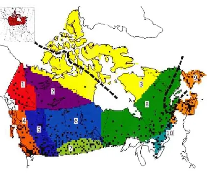
WCRDRA, 6-NWFOR, 7-NPLNS, 8-NEFOR, 9-MRTMS and 10-GRTLKS. Each of the EARCT and NEFOR regions are divided into two sub-regions, i.e. (EARCTl and EARCT2) and (NEFORI and NEFOR2), respectively. These divisions are shown by dotted lines; the region above (below) the dotted line is EARCT 1 (EARCT2) and the same description is applicable for NEFOR region. Black squares conespond to spatial distribution of CR CM grid ceUs, where at least one observation station is found. Experimental domain of the CRCM is shown in
the inset. 39
Figure 2.2 Comparison of regional growth curves for 1-, 3- and 7-day annual (April September) maximum precipitation amounts, derived from the observed data, validation simulation (VS) and reference simulations (CI-CS), for six selected regions. The plots are developed on Gumbel probability paper, wherein the inner scale along the x-axis shows retum periods. The best fitting regionaJ distribution is
indicated in each panel. 40
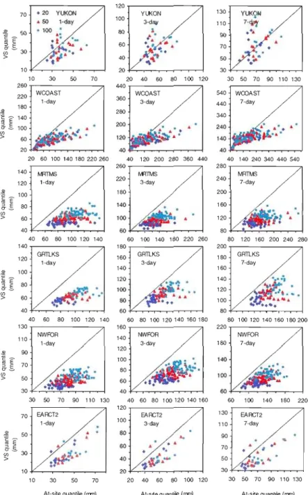
Figure 2.3 Scatter plots of 20-,50- and 100-year return levels/quantiles of 1-, 3- and 7-day precipitation extremes derived from observations (shown along the x-axis) and validation simulation (VS) (shown along the y-axis) for the period 1961-1990.
Results for six selected regions are shown only 41
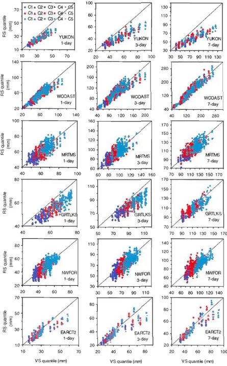
Figure 2.4 Scatter plots of 20- (dark blue), 50- (red) and 100-year (Iight blue) retum levels/quantiles of 1-, 3- and 7-day precipitation extremes derived from the validation (shown along the x-axis) and reference (CI-CS) simulations (shown along the y-axis) for the peliod 1961-1990 for six selected regions .42
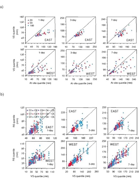
Figure 2.5 (a) Scatter plots of 20-,50- and 100-year retum levels/quantiles of 1-, 3- and 7-day precipitation extremes derived from observations (shown along the x-axis) and validation simulation (VS) (shown along the y-axis) using the GBA approach for the period 1961-1990, considering only those grid ceUs where at least two precipitation recording stations are found; (b) scatter plots of 20- (dark blue), 50 (red) and 100-year (Iight blue) retum levels derived from the VS and reference simulations (CI-CS) for the period 1961-1990. EAST refers to GRTLKS, MRTMS, NEFORI and NEFOR2 regions, white WEST refers to WCOAST and
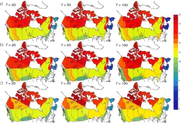
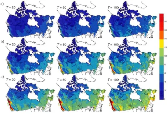
Figure 2.6 Spatial distributions of regional level 20-year (left column), 50-year (nùddle column) and 100-year (right column) return levels of (a) I-day, (b) 3-day and (c) 7 day precipitation extremes for the reference (1961-1990) period. A common
legend (in mm) is used for ail these plots 44
Figure 2.7 Spatial distribution of percentage change (increase/decrease) in 20-year (left column), 50-year (nùddle column) and 100-year (right column) regional return levels for (a) I-day, (b) 3-day and (c) 7-day precipitation extremes .45
Figure 2.8 Spatial distributions of 20-, 50- and 100-year return levels of 1-,3- and 7-day precipitation extremes at the CRCM grid-cell level, for the reference (1961-1990) period obtained using the RFA approach. Remaining notation is the same as in
Figure 2.6 46
Figure 2.9 Spatial distribution of percentage change (increase/decrease) in 20-year (left column), 50-year (nùddle column) and 100-year (right column) return levels of (a) l-day, (b) 3-day and (c) 7-day precipitation extremes at the CRCM grid cellievel
obtained using the RFA approach 47
Figure 2.10 Spatial distributions of ensemble averaged 20-, 50- and 100-year return levels of 1-, 3- and 7-day precipitation extremes at the CRCM grid-cell-scale for the reference (1961-1990) period, obtained using the GBA approach. Remaining
notation is the same as in Figure 2.6 .48
Figure 2.11 Spatial distribution of percentage change (increase/decrease) in 20-year (left column), 50-year (rniddle column) and 100-year (right column) return levels of (a) I-day, (b) 3-day and (c) 7-day precipitation extremes at the CRCM grid ceJllevel
obtained using the GBA approach .49
Figure 2.12 Regional scale 20-, 50- and 100-year return levels of 1-, 3- and 7-day precipitation extremes for the CI-CS (fi lied blue symbols) and FI-F5 (unfilled red symbols) simulations. Vertical bars are the 95% confidence intervals obtained using the vector block bootstrap resampling approach and the test-inversion method. In each pentad, plots from left ta right respectively correspond to CI-CS simulations and the same description is applicable for FI-F5 simulations 50
Figure 2.13 Regional scale 20-, 50- and 100-year return levels of 1-, 3- and 7-day precipitation extremes for the CI-CS (filled blue symbols) and FI-F5 (unfilled red symbols) simulations. Vertical bars are the 95% confidence intervals obtained using the vector block bootstrap resampling approach and standard elTor-based method. Tn each pentad, plots from left to right respectively correspond to CI-C5 simulations and the same descliption is applicable for FI-F5 simulations 51
Figure A. 1 Comparison of regional growth curves for 2-, 5- and lO-day an nuaI (April September) maximum precipitation amounts, derived from the observed data, validation simulation (VS) and reference simulations (C I-CS), for six selected regions. The plots are developed on Gumbe1 probability paper, wherein the inner scale along the x-axis shows return periods. The best fitting regional distribution is
indicated in each panel. 60
Figure A. 2 Comparison of regional growth curves for 1-, 3- and 7-day annual (April September) maximum precipitation amounts, derived from the observed data, validation simulation (VS) and reference simulations (C 1-CS), for six regions not
shown in the article. . 61
Figure A. 3 Comparison of regiona1 growth curves for 2-, 5- and 10-day annual (April September) maximum precipitation amounts, derived from the observed data, validation simulation (VS) and reference simulations (C 1-CS), for six regions not
shown in the article. .. 62
Figure A. 4 Scatter plots of 20-, 50- and 100-year return levels of 2-, 5- and 10-day precipitation extremes derived from observations (shown along the x-axis) and validation simulation (VS) (shown along the y-axis) for the period 1961-1990. Results for the six regions selected for the article. .. 63 Figure A. 5 Scatter plots of 20-, 50- and 100-year return levels of 1-, 3- and 7-day
precipitation extremes derived from observations (shown along the x-axis) and validation simulation (VS) (shown along the y-axis) for the period 1961-1990. Results for the six selected regions not shown in the article figures. . 64 Figure A. 6 Scatter plots of 20-, 50- and 100-year return levels of 2-, 5- and 10-day precipitation extremes delived from observations (shown along the x-axis) and validation simulation (VS) (shown along the y-axis) for the period 1961-1990. Results for six regions not shown in the article figures. . 65 Figure A. 7 Scatter plots of 20- (dark blue), 50- (red) and 100-year (light blue) retUll1 levels
of 2-, 5- and lO-day precipitation extremes derived from the validation (shown along the x-axis) and reference (Cl-CS) simulations (shown a10ng the y-axis) for
the period 1961-1990 66
Figure A. 8 Scatter plots of 20- (dark blue), 50- (red) and 100-year (light blue) retUll1 levels of 1-,3- and 7-day precipitation extremes derived from the validation (shown along the x-axis) and reference (Cl-CS) simulations (shown along the y-axis) for the period 1961-1990. These regions are nol shown in the article figures. . 67 Figure A. 9 Scatter plots of 20- (darl< blue), 50- (red) and 100-year (light blue) retUll1 levels
the x-axis) and reference (Cl-CS) simulations (shown along the y-axis) for the period 1961-1990. These regions are not shown in the article figures 68 Figure A. 10 Spatial distributions of regional level 20-year (left colurnn), SO-year (middle
colurnn) and 100-year (right colurnn) return levels of (a) 2-day, (b) S-day and (c) 10-day precipitation extremes for the reference (1961-1990) period. A common
legend (in mm) is used. . 69
Figure A. Il Spatial distributions of 20-, SO- and 100-year retum levels of 2-, S- and 10-day precipitation extI'emes al the CRCM grid-cell level for the reference (1961-1990) period obtained using RFA approach. A common legend (in mm) is used 70 Figure A. 12 Spatial distributions of ensemble averaged 20-, SO-and 100-year return levels of 2-, 5- and 10-day precipitation extremes at the CRCM grid-cell-scale for the reference (1961-1990) period obtained using the GBA approach. A common legend
(in mm) is used 71
Figure A. 13 Spatial distribution of percentage change (increase/decrease) in 20-year (left column), SO-year (middle colurnn) and 100-year (right colurnn) regional return levels for (a) 2-day, (b) S-day and (c) lO-day precipitation extremes 72 Figure A. 14 Spatial distribution of percentage change (increase/decrease) in 20-year (left
colurnn), SO-year (middle column) and 100-year (right column) return levels of the (a) 2-day, (b) S-day and (c) 10-day precipitation extremes at the CRCM grid cell
level obtained using RFA approach 73
Figure A. lS Spatial distribution of percentage change (increase/decrease) in 20-year (left colurnn), SO-year (middle column) and lOO-year (right colurnn) return levels of (a) l-day, (b) 3-day and (c) 7-day precipitation extremes at the CRCM grid celilevel
obtained using the GBA approach 74
Figure A. 16 Difference (in mm) between future and reference period of (a) 1-day, (b) 3-day and (c) 7-day precipitation extremes. 20-year (left colurnn), SO-year (middle colurnn) and lOO-year (right colurnn) regional return levels 7S Figure A. 17 Difference (in mm) between future and reference period of (a) 2-day, (b) S-day and (c) 10-day precipitation extremes. 20-year (left colurnn), SO-year (middle colurnn) and 100-year (right column) regional return levels 76 Figure A. 18 Difference (in mm) between future and reference period 20-year (left colllmn), SO-year (middle colurnn) and 100-year (right colurnn) return levels (obtained using the RFA approach) of (a) 1-day, (b) 3-day and (c) 7-day precipitation extremes at
the CRCM grid-cell level. 77
Figure A. 19 Difference (in mm) between future and reference period 20-year (left colurnn), SO-year (middle column) and lOO-year (right colllmn) return levels (obtained using
the RFA approach) of (a) 2-day, (b) S-day and (c) 10-day precipitation extremes at
the CRCM grid-celilevei. 78
Figure A. 20 Difference (in mm) between future and reference period 20-year (left colUInn),
SO-year (middle column) and IOO-year (right column) retlll1l levels (obtained using the GBA approach) of (a) l-day, (b) 3-day and (c) 7-day precipitation extremes at
the CRCM grid-cell level. 79
Figure A. 21 Difference (in mm) between future and reference period 20-year (left colllmn),
SO-year (middle colllmn) and 100-year (right column) retUl1l levels (obtained using
the GBA approach) of (a) 2-day, (b) S-day and (c) lO-day precipitation extremes al
the CRCM grid-celilevei. 80
Figure A. 22 Difference (in %) between delta percentages between the RFA at grid-cell level
and the GBA approaches for (a) I-day, (b) 3-day and (c) 7-day precipitation extremes of 20-year (left column), SO-year (middle column) and 100-yeaJ (right
colllmn) retUl1l levels 81
Figure A. 23 Difference (in %) between delta percentages between the RFA at grid-celilevei
and the GBA approach for (a) 2-day, (b) S-day and (c) 10-day precipitation
extremes of 20-year (left column), SO-year (middle column) and 100-year (right
column) return levels 82
Figure A. 24 Regional scale 20-, 50- and 100-year return levels of 1-, 3- and 7-day
precipitation extremes for the Cl-CS (filled blue symbols) and F l-FS (unfilled red
symbols) simulations. Vertical bars are the 9S% confidence intervals obtained using
the vector block bootstrap resampling approach and the test-inversion method. In
each pentad, plots from left to right respectively correspond to Cl-CS simulations
and the same description is applicable for FI-FS simulations 83
Figure A. 2S Regional scale 20-, SO- and 100-year return levels of 1-, 3- and 7-day
precipitation extremes for the Cl-CS (filled blue symbols) and Fl-fS (unfliled red
symbols) simulations. Vertical bars are the 9S% confidence intervals obtained using
the vector block bootstrap resampling approach and the standard error based
method. In each pentad, plots from left to right respectively correspond to Cl-CS
LISTE DES TABLEAUX
Tableau Page
Table 2. 1 Percentage of 95% confidence interval comparisons wherein changes in 20-, 50 and 100-year regional-scale return levels of 1-,3- and 7-day precipitation extremes
are found statistically significant. 53
Table B. 1 Description of the CRCM simulations used in the study 86
Table B. 2 Best fitting rank of the five candidate distributions and values of the regional
homogeneity measures Hl, H2 and H3-test 87
Table B. 3 Best fitting rank of the five candidate distributions and values of the regional
homogeneity measures Hl, H2 and H3-test 88
Table B. 4 Average boundary forcing and performance en'ors in 20-, 50- and 100-year retum levels for the Regional Frequency Analysis (RFA) method 89 Table B. 5 Average boundary forcing and pelformance elTors in 20-, 50- and 100-year retum
AM AMNO ARP CFCAS CRCM CRCMD
ERA
GBA GCM GEV GLO GNO GPA GREHYS IPCC MITACS Annual Maximum Amérique du NordAreal Reduction Factor
Canadian Foundation for Climate and Atmospheric Sciences
Canadian Regional Climate Model
Canadian Regional Climate Modelling and Diagnostics Network
European Centre for Medium-Range Weather Forecasts Re-Analysis
Grid-Box Analysis
Global Climate Model
Generalized Extreme Value
Generalized Logistic
Generalized Normal
Generalized Pareto
Groupe de recherche en hydrologie statistique
Intergovernmental Panel on Climate Change
MRC Modèle Régional du Climat
MRCC Modèle Régional du Climat Canadien
PE3 Pearson Type 3
RS Reference Simulation
RFA
Regional Frequency AnalysisRCM Regional Climate Model
UQAM Université du Québec à Montréal
B Number of bootstrap resamples
Bootstrap residuals
Heterogeneity measure
T
Standard error of y
i-th sample I-moments
Sample L-coefficient of variation
Sample L-skewness
Sample L-kurtosis
yT
Estimate of the T-year regional growth factorz
Z goodness-of-fit testa
Significance levelL-mean
L-standard deviation
k Shape parameter
F(x) Cumulative distribution function
<Il (x) Standard normal cumulative distribution function
G(x,a.) Incomplete ganuna integral
Les changements de l'intensité et de la fréquence des extrêmes hydro-climatiques peuvent avoir des impacts significatifs sur les secteurs liés aux ressources en eau. Tl est donc nécessaire d'évaluer leur vulnérabilité face aux changements climatiques.
Cette étude porte sur l'estimation des changements de la fréquence et l'amplitude des événements de précipitations extrêmes au Canada en utilisant un ensemble de dix simulations de 30 ans effectuées avec le Modèle Régional Canadien du Climat (MRCC), pour une période de référence (1961-1990) et une période future (2040-2071). Les simulations futures utilisent le scénario A2 du SRES. Deux méthodes sont utilisées dans cette étude, avec l'hypothèse de stationnarité tranche de temps (en anglais «time-slice stationarity assumption»): Analyse Fréquentielle Régionale (RFA pour «Regional Frequency Analysis»), qui s'opère à l'échelle des unités statistiquement homogènes des régions climatiques prédéfinies, avec la possibilité de réduction au niveau du point de grille et l'analyse individuelle de point de grille (GBA pour «Grid-box analysis»). Des données d'observations réhabilitées et homogénéisées de 495 stations situées partout au Canada sont utilisées pour vélifier J'homogénéité statistique des régions climatiques canadiennes. Ces données sont également utilisées pour sélectionner la distribution régionale la plus appropriée parmi les cinq distributions candidates aux trois paramètres de la modélisation observée de l, 2, 3, S, 7 et 10 jours AM (AM pour «Annual Maxima») de la quantité de précipitations (i.e. les extrêmes d'un seul jour et de plusieurs jours), survenues entre les mois d'avril et de septembre, pour la période de 30 ans allant de 1961 à 1990. Les distributions candidates sont les suivantes: la distribution des valeurs extrêmes généralisées (GEV pour «General Extreme Value»), Pareto généralisée (GPA pour «Generalized Pareto»), Logistique généralisée (GLO pour «Generalized Logistic»), Pearson Type 3 (PE3 pour «Pearson Type 3») et Normal généralisée (GNO pour «Generalized Normal»). La validation du modèle de simulation pour les périodes de retour de 20,50 et 100 ans des précipitations extrêmes d'une et de plusieurs journées en comparaison avec les observations durant la période 1961-1990 en utilisant les méthodes de RFA et GBA suggèrent une sous-estimation du MRCC pour une grande partie du Canada. Toutefois, le MRCC a tendance à smestimer légèrement sur la région de YUKON.
Les changements de l'amplitude et la fréquence des précipitations extrêmes d'un seul jour et de plusieurs joms au Canada sont estimés en utilisant les deux méthodes, celle de RFA et de GBA. Une estimation d'incertitude sous la forme d'intervalles de confiance des 20,50 et 100 ans de périodes de retour à l'échelle régionale des cinq paires de simulations de la période de référence et celle du future est effectuée en utilisant la méthode de bootstrap vectoriel (en anglais «nonparametric vector bootstrap resampling method») et ensuite explimé sous forme d'intervalle de confiance. Les résultats de l'étude ont des implications fortes pour des projets liés à la conception et la gestion des ressources en eau et pour estimer
INTRODUCTION
Les changements des événements extrêmes météorologiques et climatiques (par exemple les vagues de chaleur, les précipitations fortes, les sécheresses, les tempêtes hivernales, les ondes de tempête, etc.) ont des effets significatifs sur l'environnement, la société et l'économie. Le conséquences des événements extrêmes sur les changements des systèmes naturels et humains sont plus important que celles apportées pa le changements dans le moyennes climatiques (Parmesan, 2000). L'une des conclusions du quatrième rapport d'évaluation du Groupe d'Experts Intergouvernemental sur l'Évolution du Climat (IPCC,
2007) est que la confiance a augmenté quant à l'augumentation probable de la fréquence, de
l'intensité et de l'étendue des événements extrêmes au cours du 21 e siècle. Par conséquent, la
capacité de la société à gérer les risques dans divers domaines, causés par les événements
extrêmes, sera cruciale pour la résilience du développement et des conditions de vie.
De nombreuses catastrophes naturelles (inondations, glissements de terrain, etc.) à travers le monde provoqués par des phénomènes hydrométéorologiques intense amène la
communuauté scientifique à comprendre leur lien possible avec J'augmentation de l'intensité
des précipitations en raison d'activités anthropiques. Par conséquent, il est nécessaire d'étudier comment les caractéristiques des précipitations extrêmes seronl affectées par le
réchauffement planétaire dans les années à venir. Des recherches diverses (e.g. Fowler et
Hennessy, 1995; Trenberlh, 1999; Trenberth et al., 2003) ont suggéré que le réchauffement climatique entraînera une augmentation des précipitations intenses, dans la mesure où l'atmosphère plus chaude sera capable de contenir plus d'humidité et de produire un cycle hydrologique plus actif. Les simulations de modèles climatiques semblent en effet indiquer
que l'intensification du cycle hydrologique devrait se produi.re dans des conditions climatiques plus chaudes et cela pouo'ait entraîner une augmentation de l'intensité des précipitations, en particulier dans les événements extrèmes (McGuffie et al., 1999; Kharin et Zwiers, 2000; Palmer et Riiisanen, 2002; Tebaldi et al., 2006). A l'échelle mondiale, les expériences avec le Modèle Climatique Global Canadien (CGCM; Kharin et Zwiers, 2000) montrent une augmentation de 8% des périodes de retour de 20 ans des précipitations extrêmes quotidiennes de 2040 à 2060 et une augmentation de 1% des précipitations annuelles moyennes. Par conséquent, il existe un besoin et un intérêt croissants à étudier les changements des caractéristiques des précipitations extrêmes. Les informations sur les changements de l'intensité et la fréquence des précipitations extrêmes sont importantes pour une meilleure gestion des ressources en eau, pour l'amélioration des normes de conception d'ingénierie et pour assurer la sécurité des infrastructures diverses dans des conditions climatiques changeantes. L'étude présentée dans ce mémoire se focalisera sur l'estimation des changements (projetés) des caractéristiques des précipitations extrêmes au Canada en utilisant les simulations du Modèle Régional Canadien du Climat (MRCC) pour une période de référence (1961-1990) et une période future (2041-2070).
En général, les valeurs extrêmes sont décrites en termes de périodes de retour ou quantiles. Ceux-ci sont des valeurs qui excèdent, en moyenne, une fois pour un nombre d'années spécifié, communément appelée péliode de retour. L'analyse fréquentielle est souvent utilisée pour modéliser des précipitations extrêmes afin de développer des relations fréquence-amplitude. Il s'agit d'ajuster une distribution de probabilité à une série d'extrêmes observés ou à ceux provenant des sorties des modèles climatiques afin de définir des probabilités d'occurrences de certains événements d'intérêt. Les méthodes d'analyse fréquentielle pour des échantillons individuels d'extrêmes sont bien établies. Dans divers cadres météorologiques/hydrologiques, de nombreux échantillons des extrêmes pourraient être reliés par les mécanismes physiques générant les précipitations. S'il y a des similarités statistiques entre les extrêmes observés au sein d'une région climatique ou hydrologique homogène identifiée, des analyses plus exhaustives concernant les relations de fréquence magnitude sont possibles par l'analyse de l'enemble des échantillons au lieu de l'analyse individuels des échantillons. Cette approche est connue sous le nom d'analyse fréquentielle
régionale (RFA). La procédure de l'indice de crue (index-flood) de Darlymple (1960) en est un exemple. Au cours des années, l'approche RFA a été améliorée par un certain nombre de chercheurs, y compris l'évolution la plus notable par Hosking et Wallis (1997). Cette étude a pour but d'utiliser l'approche RFA et celle de l'analyse de point de grille/grid-box (GBA). Le GBA tient compte de chaque point de grille en tant qu'entité indépendante et admet une simulation par la méthode habituelle de modélaisation à site unique. L'approche régionale permet d'estimer l'amplitude des événements de précipitations d'une longue période de retour avec plus de fiabilité, tandis que le GBA montre la pelformance du MRC avec sa résolution à aire-limitée et il peut donner quelques détails spatiaux supplémentaires.
Du point de vue statistique, l'indépendance et la stationnarité sont les hypothèses essentielles qui doit avoir une analyse fréquentielle pour qu'èlle puisse se réaliser correctement. En outre, on émet souvent l'hypothèse que les données proviennent de la même distribution. L'hypothèse de l'indépendance ne peut pas être remplie dans les cas où la fréquence d'échantillonnage des données est assez élevée. En ingénierie, l'hypothèse de stationnarité est encore couramment utilisée pour de courts échantillons (ceux constitués de 20 ou 30 valeurs). Pour l'application des méthodes RFA et GBA, il est supposé que la distribution des extrêmes ne change pas au cours du temps durant les périodes 1961-1990 et 2041-2070, c.-à-d. qu'une stationnarité par tranche de temps (en anglais «timeslice stationarity») est supposée. De plus, la dépendance de série, si elle existe dans des échantillons de précipitations extrêmes d'un jour et de plusieurs jours, sera résolue en développement des intervalles de confiance, qui sont une partie essentielle de la procédure d'analyse fréquentielle. Cela peut être effectué en utilisant les approches appropriées telles que les méthodes de bootstrap rééchantillonnage par bloc (en anglais «block bootstrap resampling») (Khaliq et al., 2009). Par conséquent, l'influence de la corrélation sérielle n'est pas considérée explicitement lorsque des approches RFA et GBA sont appliquées aux précipitations extrêmes observées et modélisées.
Dans cette étude, les régions climatiques du Canada de Plummer et al. (2006) sont adoptées comme base pour élaborer l'approche RFA. L'analyse d'homogénéité statistique de
ces régions est effectuée en utilisant la méthodologie proposée par Hosking et Wallis (1997) et en utilisant la base de données observées des précipitations réhabilitée et homogénéisée d'Environement Canada (Mekis et Hogg, 1999; Vincent et Mekis, 2009). Il est important de noter que dans cette base de données de haute qualité le réseau de stations dans les régions centre-est et du nord est nettement moins dense que dans les autres régions du pays. Ainsi, le nombre limité des stations d'observation exclut des analyses d'homogénéité statistique fiables pour ces régions.
Les modèles climatiques constituent un des moyens pour étudier les changements de précipitations extrêmes. De nombreuses études ont examiné les changements dans les précipitations extrêmes dans des scenarios de croissance de gaz à effets de serre en utilisant les Modèles Climatiques Globaux (MCG) (e.g. Zwiers et Kharin, 1998; McGuffte et al., 1999; Tebaldi et al., 2006) ainsi que les Modèles Climatiques Régionaux (MRC) (par exemple, Fowler et al., 2005; Ekstrbm et al., 2005; Beniston et al., 2007; Mailhot et al., 2007). Cependant, il est important de noter que la précipitation est un processus atmosphérique particulièrement complexe à modéliser. En effet, la modélisation doit reposer à reproduire exactement les processus physiques complexes tels que la micro-physique des nuages, la convection, la turbulence au seuil de la couche limite planétaire et les circulations
à grande échelle. Les modèles climatiques simulent des précipitations à travers deux mécanismes principaux: les systèmes de précipitations synoptiques (ou stratiformes) et les systèmes de précipitations convectives. La précipitation à grande échelle se produit à la suite d'un soulèvement vertical de l'air lié au développement des systèmes de basse pression et des circulations orographiques ou de mousson, tandis que la precipitation convective est due à un soulèvement plus vigoureux de l'air, par exemple par le dégagement de chaleur latente. Les approches adoptées pour modéliser des systèmes de précipitations d'échelle synoptique peuvent être considérées comme plus simple que celles des systèmes convectifs. Ainsi, les différents types de paramétrage utilisés dans les modèles climatiques pour simuler ces processus physiques complexes peuvent influencer les mécanismes de précipi tations extrêmes.
De nos jours, les MRC (pilotés par les MCG) constituent des outils pertinents pour l'étude des changements d'événements de précipitations extrêmes. La résolution grossiere de MCG est moins appropriée pour l'analyse des changements de précipitations extrêmes, puisque les systèmes responsables sont généralement plus petits dans l'étendue spatiale que la résolution du MCG. Par contre, les MRC fournissent une information spatiale et temporelle de haute résolution qui améliore l'estimation des changements spatiaux et temporels des précipitations extrêmes. L'information des changements climatiques des MRC est nécessaire pour les études d'impact dans des secteurs comme l'agriculture, l'énergie, les ressources en eau, la santé et l'assurance. Toutefois, il existe de nombreuses sources d'inceltitudes associées aux modèles climatiques qui doivent être prises en compte: les incertitudes associées au développement de scénario de gaz à effet de serre, les erreurs de performance (en raison de la dynamique interne et du paramétrage du modèle), les eneurs de pilotage (en raison du pilotage de circulation à grande échelle des MCG), etc.
Les observations sont recueillies sur des sites spécifIques, tandis que les valeurs des précipitations de point de grille des modèles climatiques sont censées représenter des moyennes spatiales et donc la moyenne des précipitations pour une région sera toujow's moindre que la précipitation estimée en un point (e.g. Osborn et Hulme, 1997). Pour aborder ce sujet, des coefficients d'abattement (ARF pour «Areal reduction factors») sont nécessaires pour relier les précipitations en un point de grille à la moyenne des précipitations spatiales. Toutefois, comme il n'existe pas une compréhension claire et un consensus sur la façon dont cette relation devrait être élaborée pour les précipitations à l'échelle des points de glille simulés par les MRC et les MCG, aucune considération explicite n'est donnée aux ARP dans les analyses présentées dans cette étude.
Après la validation des précipitations extrêmes simulées par le MRC et le calcul des périodes de retour, la dernière étape nécessaire consiste à estimer l'incertitude des périodes de retour. Une estimation d'incertitude dans les prévisions de période de retour donne une certaine confiance dans leur utilisation à des fins de conception. La mesure de l'incertitude est souvent exprimée sous forme d'un intervalle de confiance pom l'estimation de quanti le.
Dans cette étude, les intervalles de confiance sont calculés en utilisant la méthode de bootstrap vectoriel (en anglais «nonparametric vector bootstrap resampling») (Efron et Tibshirani, 1993; GREHYS, 1996; Davison et Hinkley, 1997; Khaliq et al., 2009). L'avantage de cette approche par bootstrap est qu'il évite la nécessité de faire des hypothèses de distribution sur les échantillons des extrêmes pour calculer les intervalles de confiance.
Pour résumer, cette étude examine les changements à 1, 2, 3, 5, 7 et 10 jours des quantités de précipitations annuel maximales (AM) (i.e. extrêmes d'un seul jour et de plusiems joms), pour la période Avril-Septembre, en appliquant l'approche RFA basée sm les L-moments et l'approche GBA à un ensemble d'intégrations du MRCC de quatrième génération pour la période de référence (1961-1990) et les climats futurs (2041-2070). Dans cette étude, un ensemble de dix simulations de 30 ans du MRCC est considéré, cinq correspondent à la période de référence (1961-1990) et les cinq autres à la période future (2041-2070). Le MRCC est piloté par le Modèle Climatique Global (MCCG3; McFarlane et al., 2005) suivant le scénaIio «observé du 20è siècle» du GIEC (IPCC, 2001) pour la période de référence et selon le scénario A2 du Rapport Spécial sur les Scénarios d'Emission (SRES pour Special Report on Emissions Scenario; IPCC, 2001) pour la période futme. Toutes les simulations du MRCC sont effectuées avec une résolution horizontale de 45 km vrai à60° N sur une grille couvrant l'Amerique du Nord (identifié par AMNO). Pom la simulation de validation et pour la période 1961-1990, le MRCC a été pilotée par les réanalyses ERA-40 (Uppala et al., 2005).
Objectifs principaux de l'étude sont de:
1) Analyser l'homogénéité statistique des régions climatiques du Canada prédéfinies et adoptées par Plummer et al. (2006), en utilisant la base de données observeés de précipitations réhabilitée et homogénéisée par Environnement Canada (Mekis et Hogg, 1999), ainsi que l'identification des distributions régionales les plus appropriées à partir d'un ensemble de cinq distributions à trois paramètres (i.e. la distribution des valeurs extrêmes généralisées (GEV), Pareto Généralisée (GPA), Logistique Généralisée (GLO), Pearson Type
3 (PE3) et Normal Généralisée (GNO)) pour la modélisation des précipitations extrêmes d'un seul jom et de plusieurs jours.
2) Étudier les caractélistiques statistiques des précipitations extrêmes provenant des bases de données d'observation pour la période 1961-1990 et celles issues des simulations du MRCC pour la période de référence (1961-1990) et la période future (2041-2070).
3) Valider le MRCC en utilisant les approches RFA et GBA en ce qui concerne la performance et les erreurs de pilotage (en anglais «boundary forcing errors»)
4) Estimer les changements prévisionnels à 20, 50 et 100 ans de périodes de retour des précipitations extrêmes des conditions climatiques du futur (2041-2070), considerant une période de référence (1961-1990), des conditions climatiques, en utilisant un ensemble de simulations du MRCC.
5) Fournir des estimations de l'incertitude des périodes de retour régionaux sélectionnées, sous forme d'intervalles de confiance, en utilisant la méthode de bootstrap vectoriel.
6) Discuter des implications des résultats obtenus pour le Canada à l'échelle régionale et nationale.
Organisation du mémoire:
L'introduction est présentée dans ce chapitre, suivie par le Chapitre II, qui est sous forme d'un article rédigé en anglais et qui représente le cœur du mémoire. Dans cet article, divers éléments du travail de recherche sont présentés et discutés, i.e. (1) le contexte et la problématique de l'étude, (2) la bibliographie utilisée, (3) la description des régions climatiques du Canada, du MRCC et les simulations et la méthodologie adoptée et (4) les résultats obtenus. Le dernier chapitre TU contient la conclusion et la discussion des résultats. Les précipitations extrêmes de 1,2,3, 5,7 et de 10 jours de durée sont analysées pour douze régions climatiques du Canada. Dans l'article, nous présentons les résultats détaillés de 1,3 et 7 jours de précipitations extrêmes pour seulement six régions choisies. Quelques figures et tableaux de support qui ne sont pas inclus dans l'mticle, y compris des figures et tableaux se rappOltant à 2, 5 et 10 jours de précipitations extrêmes pour les six autres régions, sont fournis dans les deux annexes (A et B). Pour faciliter la compréhension, un tableau est fourni
au début de chaque annexe, mettant en évidence les sections dans l'article où les figures/tableaux ont été utilisés directement ou indirectement.
CANADIAN RCM PROJECTED CHANGES TO EXTREME PRECIPITATION CHARACTERISTICS OVER CANADA
B. Mladjicl.', L. Sushama', M.N. Khaliq2, R. Laprise'
ICanadian Regional CIimate Modeling and Diagnostics Network, University of Quebec at Montreal, 201 avenue Président-Kennedy, local PK-2315, Montreal, Quebec, Canada H2X 3Y7
2Atmospheric Science and Technology Directorate, Adaptation and Impacts Research Division, Environment Canada, Place Bonaventure, North-East Tower, 800 Gauchetiere Street West, Office 7810, Montreal, Quebec H5A lL9, Canada
"CoITesponding author address: Bratislav Mladjic
Département des Sciences de la Terre et de l'Atmosphère, UQAM P. O. Box 8888, Stn Downtown
Montréal, Québec, Canada H3C 3P8 Tel: +1 (514) 928-2029
Email: [email protected]
Abstract
Changes to the intensity and frequency of hydro-climatic extremes can have significant impacts on sectors associated with water resources and therefore it is important to assess their vulnerabilities in a changing climate. This study focuses on the assessment of projected changes to the frequency and magnitude of extreme precipitation events over Canada using an ensemble of ten 30-year integrations peIformed with the Canadian Regional Climate Model (CRCM), for reference (1961-1990) and future (2040-2071) periods; the future simulations correspond to A2 SRES scenario. Two methods, the regional frequency analysis (RFA), which operates at the scale of statistically homogenous units of pre-defined climatic regions, with the possibility of downscaling to grid-cell level, and the individual grid-box analysis (GBA) are used in this study, with the time-slice stationarity assumption. Validation of model simulated 20-,50- and lOO-year return levels of 1-, 2-,3-,5-,7- and 10-dayextreme precipitation events (i.e. single- and multi-day events) against those observed for the 1961 1990 pel10d using both the RFA and GBA methods suggest underestimation by the CRCM over most of Canada. However, the CRCM tends to overestimate over the Yukon region. The CRCM projected changes to selected return levels for the future (2041-2070) period in comparison to the reference (1961-1990) period suggest an increase in event magnitudes, which appear ta be significant, particularly for the western (West Coast, Western Cordillera), eastern (Northeast Forest) and Yukon Territory, Mackenzie Valley and Arctic regions as weil as for the Northwest Forest Prairie region. 10 general, positive but relatively less significant changes are noticed for the Great Lakes, Maritimes and Prairie (Northern Plains) regions. The results of the study have strong implications for both design and management of water resources related projects and for assessing sustainability of existing infrastructures in a changing climate.
Keywords: Canadian climatic regions; climate change; precipitation extremes; regional climate modelling; regional frequency analysis.
2.1 Introduction
Extreme hydro-climatic events such as precipitation extremes, floods and droughts can impact society significantly, bringing enormous environmental, social and political repercussions. In the context of a changing climate, it is therefore important to investigate changes to characteristics of these events. Hence, this study focuses on changes to characteristics of precipitation extremes only. Information about changes to intensity and frequency of extreme precipitation events is crucial for better management of water resources, developing guidelines for revising engineering design standards and ensuring safety of various infrastructure facilities under changing climate conditions.
The Fourth Assessment Report of the Intergovernmental Panel on Climate Change (IPCC, 2007) discussed changes in mean precipitation observed over recent decades for many regions of the world and suggested that it is very likely that frequency and intensity of heavy precipitation events will increase over many regions in the future.
Assessment of changes to characteristics of precipitation extremes due to variations in greenhouse gas concentrations was investigated in previous studies using global climate model (GCM) simulations (e.g. Zwiers and Kharin, 1998) as weil as using regional climate model (RCM) simulations, e.g. Fowler et al. (2005) and Ekstrbm et al. (2005) for the United Kingdom, May (2008) and Beniston et al. (2007) for Europe and Mailhot et al. (2007) for southern Quebec. At the present point in time, RCMs offer the best information with respect to GCM, for studying changes to extreme precipitation events. Theil' advantage over the GCM is that they provide highly resolved spatial and temporal information that enhances assessment of spatial and temporal changes to extreme precipitation.
Extreme values are usually described in tenns of retum Ievels or quanti les. These are the values that are exceeded, on average, once every specified number of years. Return levels are generally computed by fitting a parametric distribution to a sample of annual maximum (AM) or peaks-over-threshold (POT) values. In the former method, which is very commonly
used because of its simple structme, only one value from each year/season is considered and in the latter, more than one value pel' year/season could be considered. Since extreme events are rare and historical records are often short, estimation of frequencies of extreme events is a challenging task. When data at a given location are insufficient for a reliable estimation of quantiles, regional frequency analysis (RFA) could be a useful alternative. The RFA has been an established method in hydrology for many years and it is also becoming popular in climatology because of its advantage mentioned above. Il is often remarked thar the RFA method substitutes space for time by using observations from different sites in a region to compensate short records at individual sites.
This study investigates changes to 1-, 2-, 3-, 5-, 7- and lO-day AM precipitation amounts, for the April-September period, applying the L-moments based RFA approach of Hosking and Wallis (1997) to an ensemble of the fourth generation Canadian RCM (CRCM) integrations for the reference (1961-1990) and future (2041-2070) climates. As a complementary approach to RFA, grid-box analysis (GBA), which opera tes on individual grid cells of the CRCM, is also peIformed. Rehabilitated and homogenized precipitation records of 495 stations from Environment Canada, located across Canada (Vincent and Mekis, 2009), is used for evaluating the CRCM perfolmance for the period 1961-1990. For a successful implementation of the RFA approach, observational sites or grid boxes must be assigned to statistical homogeneous regions, since approximate homogeneity is required to ensure that RFA is more robust than an at-site analysis (Hosking and Wallis, 1997). Identification of homogeneous regions is usually the first and the most difficult task in RFA as it may involve many subjective decisions (GREHYS, 1996). For the purpose of this study, previously defined Canadian climatic regions from Plummer et al. (2006) are adopted as the basis for developing RFA approach. These climatic regions are tested for their statistical homogeneity and divided further into smaller sub-regions where necessary by maintaining the notion of contiguous homogeneous regions. Since 30 years long reference and future periods are located over sufficiently separated disjoint time intervals, time-slice stationarity for both the reference and future climate conditions is assumed for the analyses presented in this paper.
The paper is organized as follows. A brief description of the CRCM and its simulations used in the analysis are given in Section 2. Description of the Canadian climatic regions along with details of the observational records is provided in Section 3. Section 4 contains a description of the methodology used for estimating changes to extreme precipitation events. Detailed results of the CRCM validation and projected changes to precipitation extremes are presented in Section 5, followed by discussion and main conclusions of the study in Section 6.
2.2 Model and simulations
The model used in this study is the latest operation al version of the CRCM (version 4.2.3), i.e. the fourth generation of the CRCM. A detailed description of the earlier versions of the CRCM can be found in Caya and Laprise (1999) and in Plununer et al. (2006). The CRCM's horizontal grid is uniform in polar stereographic projection and its vertical resolution is variable with a Gal-Chen scaled-height terrain following coordinate. In the most recent version, sub-grid scale physical parameterization largely follows the Canadian General Circulation Model Version III (CGCM3) physics (Scinocca and McFarlane, 2004; McFarlane et al., 2005), that is adapted to the regional modeI's grid and projection.
An ensemble of ten 30-year CRCM integrations are considered in this study, of which five correspond to the CUITent climate (1961-1990) reference period and the other five are the matching simulations for the future (2041-2070) period. The CRCM peliorms dynamical downscaling of different members of an ensemble of CGCM3 simulations to produce climate projections at the regional scale following IPCC "observed 20th century" scenario (IPCC, 2001) for the reference and Special Report on Emissions Scenarios (SRES) A2 scenario (IPCC, 2001) for the future. In addition, a validation run spanning the 1961-1990 period, where the CRCM is driven by ERA4ü (Uppala et al., 2005) is considered and will be referred to as "validation simulation" or simply VS hereafter. Ali CRCM simulations are performed at a horizontal resolution of 45 km true at 600
N over a North-American domain shown in Fig. 2.1. For the convenience of presentation, the five CGCM3 driven simulations for 1961-1990 are refened to as Cl, C2, C3, C4 and C5, while corresponding simulations for 2041-2070 are
referred to as FI, F2, F3, F4 and F5 in this paper; together, these Cl-C5 and Fl-F5 simulations are respectively refelTed to as "reference simulations" and "future simulations".
2.3 Description of Canadian climatic regions and observational records
2.3.1 Climatic regions
A set of 10 predefined clirnatic regions is adopted from Plummer et al. (2006) for the purpose of this study. The northern regions include YUKON (Yukon Territory), MACK (Mackenzie Valley) and EARCT (East Arctic), the regions over the western Canada and Prairies are the WCOAST (West Coast), WCRDRA (Western Cordillera), NWFOR (Northwest Forest), and NPLNS (Northern plains), the eastern regions are the NEFOR (Northeast forest), GRTLKS (Great Lakes) and MRTMS (Canadian Maritimes). The WCOAST, WCRDRA, NPLNS and GRTLKS regions are spread over the Canadian and the US telTitory, however, only the Canadian portion of these regions is retained, as this study focuses on Canada. These climatic regions are shown in Fig. 2.1.
2.3.2 Observational records
Observational records consist of 495 stations included in the rehabilitated and homogenized precipitation database of Canada. This database was developed by applying adjustments for known reasons of non-homogeneity, e.g. changes in instrument type, station relocations, trace biases, etc. (Vincent and Mekis, 2009). Most of the records are available till 2007 and for some stations records go as far back as 1900. Data availability in much of the Canadian Arctic is restricted to 1948-2007. Spatial distribution of the CRCM grid cells containing at least one station out of 495 stations is shown in Fig. 2.1. It is clear from this figure that most of the stations are concentrated in southern parts of the country, along the border with the US. Central, east-central and northem regions have significantly less dense network of stations. This is an obvious linùtation of the rehabilitated and homogenized database. This database is used for verifying statistical homogeneity of Canadian climatic regions, discussed in the previous section, and for selecting the most appropriate regional distlibution for modelling observed 1-,2-,3-,5-,7- and lO-day AM precipitation, occurring
over the April to September months, for the 30-year period from 1961 to 1990 in an RFA setting, described in detail in the section to follow. The April to September period is chosen to avoid mixing of snow and rainfall extremes. To a greater extent, this time window helps to maintain homogeneity of the samples of precipitation extremes from a physical viewpoint as weil as to preserve their seasonality. As the reliability of the analyses is highly dependent on the quality as weil as on the completeness of records, a year with more than five missing daily values is considered a missing year and only those stations with at least 21 val id years are considered for the analyses. Though the records are available for time periods longer than 30 years, the 1961-1990 time window is chosen in order to match the CRCM refel'ence period described earlier. The total number of available stations and those retained for analysis following the missing value and station inclusion criteria (given in brackets) are 21 (15) for YUKON, 16 (9) for MACK, 39 (33) for EARCT, 66 (58) for WCOAST, 65 (59) for WCRDRA, 58 (53) for NWFOR, 46 (43) for NPLNS, 86 (73) for NEFOR, 63 (59) for MRTMS and 35 (30) for GRTLKS regions. ln total, the number of stations considered for analysis in this study is 432 out of 495.
2.4 Methodology
Two complementary methods are used to assess the CRCM pelfol'mance and projected changes to frequency and magnitude of extreme precipitation events over Canada: the RFA and GBA. For the application of these two methods it is assumed that the distribution of extremes does not change ovel' time during the periods 1961-1990 and 2041-2070. In other words, time, time-slice stationarity is assumed. Analyses are pelformed using 1-,2-,3-,5-,7 and 10-day obsel'ved and modeled AM precipitation amounts. The RFA approach allows estimation of desired return levels, particularly those corresponding to higher return pel'iods, with more l'eliability compared to a single site based estimation (Hosking and Wallis, 1997); analogously this remark can be extended to a single grid-cell based estimation as weil. Advantages of the RFA are especially evident when only short records are available. This assertion appears to be applicable for the present analyses because at the most 30 values pel' station or grid-cell are included in the analysis in order to be consistent with the time-slice CRCM expeliments. Compared to the RFA approach, the GBA shows perfonnance of the
CRCM at grid-cell scale and hence it could provide more detailed spatial information. The usefulness of the RFA and the GBA approaches have been investigated in a few recent studies on modeling regional c1imate model simulated precipitation extremes, e.g. Fowler et al. (2005), Ekstrbm et al. (2005) and Mailhot et al. (2007).
The CRCM perlormance and boundary forcing errors (Sushama et al., 2006) are assessed: pelformance errors are due to the internaI dynamics and physics of the regional model and boundary forcing errors are due to the errors present in the driving data. Comparison of selected observed return levels with those from the validation simulations for the period 1961-1990 is used to assess perlormance errors. Comparison of selected return levels from the validation and reference simulations provide assessment of boundary forcing enors. This validation is perlormed using both the RFA and GBA approaches. Assessment of the performance of the CRCM is followed by an analysis of the CRCM reference and futme period integrations, in order to study changes to characteristics of extreme precipitation events over Canada.
2.4.1 The L-moments based RFA approach
In general, there are two main steps involved in an RFA approach: (1) identification of suitable statistical homogeneous regions and (2) selection of an appropriate regional distlibution to generate regional growth curves or factors. A regional growth curve represents a dimensionless relationship between frequency and magnitude of extreme values. In this study, a standard RFA approach based on L-moments of Hosking and Wallis (1997) is used to generate regional growth curves for the observed data and validation (V S), reference (C 1
CS) and futme (F1-Fs) integrations. In theory, L-moments characterize a wider range of distributions and they are believed to be more robust to the presence of outliers (Hosking and Wallis, 1997). Because of this reason, the estimators based on L-moments tend to be less biased compared to product moment based estimators. Also, L-moments based estimators are sometimes more accurate for smail samples than those obtained using the maximum likelihood procedures (Hosking, 1986). A brief description of the sample L-moments required for the analysis of observed and simulated extremes and that of the theoretical L
moments, along with the selected candidate distributions, is provided in Appendix A. Candidate distributions include the Generalized Extreme Value (GEV), Generalized Pareto (GPA), Generalized Logistic (GLO), Pearson-Type 3 (PE3) and Generalized NOimal (GNO). For a single site or a single grid-cell, parame ter estimation for any candidate distribution is pelformed by equating sample L-moments (more preferably their ratios) to their theoretical counterparts and solving the resulting equations directly or through iterative numerical algorithms. For the RFA approach, sample size-weighted averaged values of L-moment ratios are used for parameter estimation of the candidate distributions.
For verifying statistical homogeneity of Canadian climatic regions and their subdivision into smaller homogeneous regions, regional homogeneity tests based on L moment ratios are used. According to Hosking and Wallis (1997), heterogeneity measures for
a region are based on values of Hl, H2 and H3, where Hl, H2 and H} are weighted standard
deviations of (i) L-coefficient of variation, (ii) L-skewness and (iii) L-kurtosis, respectively. These measures are derived using Monte Carlo simulations. A region may be regarded as
"acceptably" homogenous for H values below 1, "possibly" heterogeneous for H values
between 1 and 2 and "definitely" heterogeneous for H values equal and above 2. For regions
with H values greater than 2, a further subdivision into smaller regions is undeltaken with the
objective of improving on quanti le estimates. This subdivision is undertaken using the cluster analysis algorithm (Hosking and Wallis, 1997) if this analysis resulted in meaningful contiguous subdi visions.
In order to select an appropriate regional distribution from the GEV, GPA, GLO, PE3
and GNO distributions for developing regional growth curves, the Z-statistic developed by Hosking and Wallis (1997) is used here. This statistic is described in Appendix B. A candidate distribution passes the Z goodness-of-fit test, for instance, at 10% significance
level, if the
1
Z DI5T1<
1.64, It is possible that more than one distribution would appearadequate following this testing procedure. In that situation and in situations where none of the
candidate distributions passed the Z test, a best candidate distribution is chosen as the one
for each statistically homogeneous climatic region, comparisons of the selected return levels obtained from observations and VS of the model for the period 1961-1990 is carried out to validate the CRCM. This validation is followed by the CRCM reference and future integrations analysis in order to study changes to extreme precipitation events in an RF A setting. Whichever is the type of the best fitting regional distribution for observed extremes, the same distribution is assumed for the analysis of extremes derived from the validation (VS) and reference (CI-C5) and future (F1-F5) integrations. This approach is followed in order to maintain distributional consistencies under the assumption that a three-parameter best fit distribution is sufficiently flexible to Jescribe changes in distributional shapes that would occur with reference and future period integrations.
2.4.2 The GBA approach
For this approach, frequency analysis is performed by considering each CRCM grid cell as an independent entity. However, the influence of spatial correlations on future Jevels is taken into account when deriving confidence intervals. Distribution fitting analysis and selection of the best fitting distribution for each grid-cell can be performed in a similar manner as for the RF A appwach described above. However, this anaJysis can only be performed for those grid cells, where an observation station is found. For the remaining grid cells, one has to subjectively assume a distribution. Aiternatively, based on a goodness-of-fit test, one could use different distribution types that cou Id vary from one grid-cell to the next and also from reference to future period integrations. The latter possibility does not seem to be 10gicaJ because of the inconsistencies arising from different distributionai types for the same grid-cell. Therefore, to avoid such problems, the overall best fitting distribution, found after implementing the RFA approach, is used for the GBA for the entire study area. Thus, for ail grid ceJls, the type of the distribution stays the same for both reference and future period integrations. Validation of the CRCM using the GBA approach is performed for only those grid cells where an observation station is found.
2.5 Results
Since statistical homogeneity of Canadian c1imatic regions is a pre-requisite for the RFA approach, results for this analysis are presented first followed by those of the CRCM validation, in terms of performance and boundary forcing errors. The CRCM validation would furnish an overview of how the model reproduces various statistical characteristics of single- and multi-day extreme precipitation events. After discussing validation of the CRCM, results for projected changes to characteristics of extreme precipitation events are presented and discussed. Though complete analyses are performed for 1-, 2-, 3-, 5-, 7- and 10-day precipitation extremes, detailed results are presented only for 1-, 3- and 7-day events. Where appropriate, results for the remaining (i.e. 2-, 5- and 10-day) extremes are also discussed.
2.5.1 Statistical homogeneity analysis of Canadian climatic regions
Statistical homogeneity of each of the predefined climatic regions, adopted from the work of Plumer et al. (2006), is exarnined, with the available number of stations which satisfy the station inclusion criteria, described earlier in the section on methodology. For this purpose, 1-, 2-, 3-, 5-, 7- and lO-day observed precipitation extremes are considered. If the calculated values of the H statistics are higher than 2 for at least three out of six cases (e.g. if
H statistics are simultaneously higher than 2 for 1-,3- and 7-day precipitation extremes) then further subdivision of the region is undertaken, conditional to a successful implementation of the cluster analysis algorithm. Seven predefined regions, i.e. the YUKON, MACK, WCOAST, NWFüR, NPLNS, GRTLKS and MRTMS pass these criteria, while the remaining WCRDRA, EARCT and NEFüR regions do not, and hence their subdivision into smaller regions is undertaken.
The WCRDRA, EARcr and NEFüR regions are found to have higher than permissible value of the HI statistic and therefore cluster analysis is performed to subdivide these three regions into sma\ler homogeneous sub-regions. Satisfactory cluster analysis is feasible for EARCT and NEFOR regions only. Hence, EARCT region is subdivided into EARcrl and EARCT2 (shown in Fig. 2.1) and NEFüR into NEFüR1 and NEFOR2 (also
shown in Fig. 2.1). It is not possible to subdivide the WCRDRA region into smaller contiguous homogeneous regions and hence this region was considered as is, despite its suspected homogeneity. Perhaps it may be possible to subdivide this region into smaller non contiguous homogeneous regions but such a subdivision is not considered since the focus of this study was to find contiguous smaller homogeneous regions within the predefined larger climatic regions of Plurnrner et al. (2006). Based on the analyses presented and discussed above, a set of 12 climatic regions (shown in Fig. 2.1) is considered for RFA of AM values of daily and multi-day precipitation events.
2.5.2 Validation of the CRCM simulations
Validation of the CRCM simulated precipitation extremes is performed using the VS for the period 1961-1990, after implementing the following three steps: (1) For ail 12 regions, observed regional growth curves are developed based on precipitation extremes of those stations that fall within each region. The observed regional growth curves are used to
develop, dimensionless growth factors for selected return periods (i.e. / values, where T is
the return period) and these factors in turn are used to estimate at-site return levels using the
at-site li values for each aggregation level considered (i.e. 1-, 2-, 3-, 5-, 7- and JO-day); (2)
Regional growth curves are developed for each region based on the simulated precipitation extremes (i.e. the ones derived from the VS) for all grid cells that faH within each region. From the regional growth curves, dimensionless growth factors for selected return periods are obtained and these growth factors in turn are used to estimate return levels for each grid-ceJI
using the corresponding II value for each aggregation level considered; (3) For each of the 12
regions, scatter plots of 20-, 50- and 100-year return levels are developed for only those CRCM grid cells where at least one station is found. Such plots are useful to examine the extent of under- or over-estimation of various quantiles and therefore help assess CRCM 'performance errors' due to the internai dynamics and physics of the regional mode!.
Observed regional growth curves are compared to those developed from model simulated extremes in Fig. 2.2 for six selected regions, i.e. YUKON, WCOAST, MRTMS,