MSE lower bounds for deterministic parameter estimation
5
0
0
Texte intégral
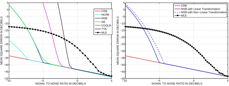
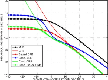
Figure
Documents relatifs
