O
pen
A
rchive
T
oulouse
A
rchive
O
uverte (
OATAO
)
OATAO is an open access repository that collects the work of Toulouse researchers
and makes it freely available over the web where possible.
This is a publisher-deposited version published in:
http://oatao.univ-toulouse.fr/
Eprints ID: 2246
To link to this article: DOI:
10.1109/SIES.2009.5196187
URL:
http://dx.doi.org/10.1109/SIES.2009.5196187
To cite this version: FERRANDIZ, Thomas, FRANCES, Fabrice, FRABOUL, Christian. A
method of computation for worst-case delay analysis on SpaceWire networks. In : IEEE
International Symposium on Industrial Embedded Systems, 2009 : SIES '09 ; 8 - 10 July
2009, Ecole Polytechnique Federale de Lausanne, Switzerland. Piscataway : Institute of
Electrical and Electronics Engineers ( IEEE ), 2009, pp. 19-27. ISBN 978-1-4244-4110-5
Any correspondence concerning this service should be sent to the repository administrator:
A method of computation for worst-case
delay analysis on SpaceWire networks
Thomas Ferrandiz
Fabrice Frances
Christian Fraboul
Univ. of Toulouse, ISAE Univ. of Toulouse, ISAE Univ. of Toulouse, ENSEEIHT/IRIT 10 avenue Edouard Belin 10 avenue Edouard Belin 2, rue Charles Camichel
BP 54032 BP 54032 B.P. 7122
31055 Toulouse Cedex 4 31055 Toulouse Cedex 4 31071 Toulouse Cedex 7
France France France
+33 5 61 33 90 97 Email: [email protected] Email: [email protected] Email: [email protected]
Abstract-SpaceWireis a standard for on-board satellite networks chosen by the ESA as the basis for future data-handling architectures. However, network designers need tools to ensure that the network is able to deliver critical messages on time. Current research only seek to determine proba-bilistic results for end-to-end delays on Wormhole networks like SpaceWire. This does not provide sufficient guarantee for critical traffic. Thus, in this paper, we propose a method to compute an upper-bound on the worst-case end-to-end delay of a packet in a SpaceWire network.
I. INTRODUCTION
SpaceWire ([1],[2]) is a high-speed on-board satellite network created by the ESA and the Uni-versity of Dundee. It is designed to interconnect satellite equipment such as sensors, memories and processing units with standard interfaces to encourage re-use of components across several missions.
SpaceWire uses serial, bi-directional, full-duplex links, with speeds ranging from 2 Mbps to 200 Mbps, and simple routers to interconnect nodes with arbitrary topologies.
In the future, SpaceWire is scheduled to be used as the sole on-board network in satellites. As a high-speed network with low power con-sumption, it is well-suited to this task. It will be used to carry both payload and control traffic, multiplexed on the same links. These two types of traffic have different requirements. Control traffic generally has a low throughput but very strict time constraints. On the contrary, payload traffic
does not need strict guarantees on the end-to-end delays of packets but requires the availability of a sustained, high bandwidth to be operational.
Both requirements were easy to satisfy on point-to-point SpaceWire links. But in order to connect every terminal on a single SpaceWire network, a router was designed with space con-straints in mind (especially radiation concon-straints on memory) which led to the use of Wormhole Routing.
However, the problem with using Wormhole Routing is that it can occasionally lead to long delays if packets are blocked as shown in our SpaceWire overview in Section II. Those blocking delays make it difficult to predict end-to-end delays especially when control and payload traffic are being transmitted on the same network.
This is why previous delay evaluation methods on Wormhole networks have only focused on probabilistic results which do not provide enough guarantee for network designers, who would like to be sure that control packets are always deliv-ered within an acceptable timeframe (simulations do not cover every possible case). To this end, a better approach would be to determine only an upper-bound on the worst-case end-to-end delay. As a consequence, we have designed a method of computation that enables the determination of such a bound. Section III presents this method and a demonstration on a sample network is given in Section IV. Finally, we conclude and propose future topics for research in Section V.
2
R1 R2
2
R1 R2
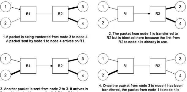
1.A packet is being tranferred from node 3 to node 4. A packet sent by node 1 to node4arrives on R1.
2. The packet from node 1 is transferred to R2 but is blocked there because the link from
R2 to node4is already in use.
R1 R2 R1 R2
3
3. Another packet is sent from node 2 to 3. It arrives in R1 and is blocked because the link R1-> R2 is in use.
4. Once the packet from node 3 to node 4 has been transferred, the packet from node 1 to node 4 is transmitted. The packet from node 2 still has to wait.
Figure 1. Packets can get blocked in a SpaceWire network II. A BRIEF DESCRIPTION OF SPACEWIRE
A. SpaceWire as a point-to-point link
Originally, SpaceWire was designed to provide only point-to-point links between satellite equip-ment. It is derived from the IEEE 1355 standard [3] but uses new connectors and cables suitable for space usage.
SpaceWire uses two types of characters as transmission units: data characters and control characters. Data characters are lO-bits long and carry one byte of data along with one parity bit and one data/control flag. Control characters are 4-bits long and contain 2 bits coding a control code, one parity bit and one data/control flag. They are used to mark the (possibly erroneous) end of packets and for flow control.
SpaceWire uses a flow control mechanism to ensure that no node receives data that could cause a buffer overflow. On each link, the emitter can only send characters if the receiver allows him to by sending a control character (Flow Control Token or FCT). Each FCT allows the emitter to send 8 characters with a maximum of 56 characters authorized at anyone time.
Data are organized in packets of arbitrary length with a very simple format. Each packet is composed of three fields: an address field, a cargo field and an End-Of-Packet marker. The address and cargo fields can be of any length and it is even possible to send packets of unlimited size.
20
SpaceWire's point-to-point links thus provide a simple and fast way to transmit data between two terminals. Furthermore, the end-to-end delay is quite simple to compute. If the source and destination do not cause delays themselves, the delay is simply ~ where T is the packet size and C the capacity of the link.
B. SpaceWire as an interconnection network
With the increasing quantities of data ex-changed by various equipment, using only point-to-point links to connect all the equipment be-comes too costly. Furthermore, in order to reduce the complexity of the on-board system, it would be better to use a single network to carry both payload and command/control traffic instead of using a dedicated bus (generally a MIL-STD-l553B bus) for the control traffic and high-speed data links for the payload traffic.
These considerations have led to the addition of routers to the SpaceWire standard, allowing the construction of networks with arbitrary topolo-gies. These routers are required to comply with two main constraints. Firstly, they must remain compatible with the point-to-point links used to interconnect equipment and secondly, they cannot use a lot of memory because radiation tolerant memory is very expensive.
As a consequence, Wormhole Routing was chosen as the way to transmit packets through the network. With this technique, instead of buffering
whole packets, a router reads a packet's header on-the-fly when it arrives. Then the router uses this information to determine the appropriate out-put port and checks the state of this port (see Figure I). If the output port is free (immediately after the packet arrives or after a delay), the packet header is transferred without waiting for the rest of the packet. This allows the routers to use only 8 to 64 bytes of buffer memory per input link. When the output port is allocated to the packet, it is marked as occupied by the router and no other packet can pass through as long as the current packet has not been completely transferred.
This means that, if the output port is already occupied by a packet, the second packet will have to wait until the first one has been transferred. Given that the flow control mechanism is active on each link, small parts of the second packet are blocked in each of the routers crossed by the packet as they wait for the head of the packet to get access to the occupied output port. In tum, they block access to all the output ports used by the packet in the above routers. When the occupied output port finally gets free, one of the blocked worms (packet) is elected, on a round-robin basis.
As can be seen, using Wormhole Routing sat-isfies both constraints cited above. Routers need little memory for each input link and no memory at all for output links. They are also backward compatible since they propagate the point-to-point SpaceWire flow control to each link along the end-to-end path, backwards from the receiver to the emitter.
However, Wormhole Routing has a major draw-back which is that packets might get blocked for a long time in routers. Two mechanisms were thus added to SpaceWire routers to offset this problem. The first is a two-level static priority scheme that is used in routers so that packets sent to a high-level address are always transmitted before packets sent to low-level addresses. As SpaceWire routers are not preemptive, the priority mechanism is only applied when two packets are waiting for the same output port to be freed. The round-robin scheme is then used to arbitrate between packets of the same priority level.
The second mechanism is called Group Adap-tative Routing. It works by putting two or more
parallel links between two routers. In this case, they're declared as a group in the routing tables and the routers are able to automatically balance the load on the multiple links. However, as it increases the number of links instead of sharing them, this mechanism should be used only for fault tolerance or if it is really impossible to transmit all the traffic on one link.
Together, these two mechanisms can reduce the blocking problem but they cannot solve it completely. Thus, in order to evaluate the end-to-end delays in a SpaceWire network, we need to be able to determine how long packets might remain blocked.
C. The end-to-end delay determination problem: related work
Optimally, a packet is not blocked in any en-countered router and endures only the switching delay of each router. The switching delay includes the time to read the header of the packet, deter-mine the output port and copy the first character to the output link. SpaceWire router specifications require the router's switching delay to be less than 0.5 J-LS when links work at 200 Mbps. This means that the delivery time of a packet across a SpaceWire network will be equal to the delivery time on a point-to-point link plus 0.5 J-LS per router crossed.
However, access conflicts can occur on each link taken by a packet. Furthermore, the packet blocking a link can in tum be blocked farther on the network. This makes it very hard to determine the end-to-end delay of a single packet analytically.
A great deal of research has been published on the estimation of end-to-end delays in Wormhole Routing networks, particularly in supercomputers. However, that research only seeks to determine average latency using techniques like queuing theory (see [4] and [5] for example). Knowledge of average latency is not sufficient here since we must be certain that all messages are delivered within an acceptable timeframe.
Network Calculus [6] is another technique that has been successfully used to evaluate bounds on worst-case end-to-end delays in embedded networks. For example, it was used in [7] to analyze a Switched Ethernet network used to re-place a MIL-STD-1553B bus in a military avionic
network. However, SpaceWire does not appear to be modelisable using classical network elements like multiplexers and buffers. Indeed, we could not model Wormhole routers using service curves because the service offered to a flow depends on the other flows in the network and on the network topology. To our knowledge, no one has done such a modelisation at the moment.
As a consequence, we propose a more practical approach which works by computing a bound on the worst-case end-to-end delay for each flow. This way, the individual delay of each packet is not characterized but the timely delivery of control traffic packets can still be guaranteed.
III. COMPUTING A BOUND ON THE WORST-CASE DELAY
A. Notations and definitions
We model a SpaceWire network as a con-nected directed graph
9(N, L).
The nodesN
of the graph represent both the terminals and the SpaceWire routers. The edges L represent the set of SpaceWire links. We use two edges in opposite directions to represent a bi-directional SpaceWire link.A communication between a source and a destination is modeled as a flow
f.
Each flowf
has a maximum packet size, noted T]. This includes the protocol headers. Each flow goes through a set of links that form a path in9
(N, L).The set of flows is denoted F. Knowing the throughput of every flow is not necessary but we make the assumption that the capacity of any link is sufficient to transmit all the data using that link. We note links(f) the ordered list of the links
the flow f follows. first(f) returns the first
link in links(f). We note next(f, l) the function
which, given a flow f and a link l in links(f)
returns the next link in links(f) right after land prev(f, l) the function returns the previous link
in links(f) just before l. If l is the last link in links(f), next(f, l) returns null. If l is the first
link in links(f), prev(f, l) returns null.
We also make the following assumptions : • the routing is static (current SpaceWire
routers use static routing anyway)
• SpaceWire's Group Adaptative Routing fea-ture is not used (thus S is not a multigraph) • all the links have the same capacity C (this is not very restrictive since reducing link speed
22
does not seem to reduce power consumption significantly)
• we do not take into accounts adresses prior-ities in the routers (i.e. all nodes have low priority adresses)
• we neglect the delays caused by Time-Codes and Flow Control Tokens (Time-Codes are special characters used by SpaceWire to syn-chronize a global clock on the network) • packets are processed as soon as they arrive
at their destination (i.e. the destination itself does not delay the packet)
• when a source starts to send a packet, it transmits it at the maximum possible speed until the entire packet has been transferred (i.e. the source itself does not delay the packet)
In order to remove the last two assumptions, we would have to model the behaviour of each node on a case-by-case basis since we do not have a generic model of the nodes at the moment.
B. The method of computation
The method of computation is based on the idea that, in a SpaceWire network, the delivery of a packet can be divided into two phases. During the first phase, the first character (the header) of the packet is routed to its destination through intermediary routers and creates a "virtual circuit" between the source and destination of the packet using Wormhole Routing. In the second one, the whole packet can be transferred along the path of the circuit, as if it were a point-to-point link. When the packet's transfer is completed, the links are freed and the "virtual circuit" disappears.
Let us consider a bound on the worst case delay for packet p of flow fp. As the source and destination of the packet do not cause any delays, only the routers crossed by p can delay it during the first phase. In each router, this delay has two possible causes. The first is the switching delay of the router and includes the time needed to determine the port through which
p will be transferred. This delay is constant for every packet and every SpaceWire router. We will note it dsw afterwards.
The second delay occurs when the output link is already in use by another packet. With Worm-hole Routing, p has to wait until the packet using the port is completely transferred. It is
also possible that one or more packets coming from other ports may already be waiting for the same output port to become free. The delays will then accumulate if those packets are transferred before p. Note that, as ports are independent in SpaceWire routers, only packets using the same output port as p can cause a delay.
SpaceWire routers use a Round Robin scheme to arbitrate between concurrent input links trying to access the same output link. Therefore, even in a worst case scenario, at most one packet from each of the other input link may be transmitted before p can be transferred.
For each of these input links, several flows can enter the router. Thus we need to compute a bound on the maximum delay that each of these flows may produce and then calculate the maximum of these potential delays.
The maximum delay that a packet q can cause
pis the time to transfer q starting from the current router if q was alone in this router (i.e. q does not have to wait for the output port to become free). However, q may in turn become blocked in the next routers it crosses by other packets.
Once it can access the appropriate output link, the header of a packet is transferred to the next router and must once again wait to access the output port it needs.
As a consequence, we can now formulate a recursive definition of an upper bound on the delay di], l) needed to deliver a packet of flow
f
starting from the moment when the packet tries to access link l with li-
null and li-
first(f) :d(f, l)
==
L [
max d(fin, next(fin, l))i. EB finEUl i n un. f,l +dsw ]
+
di],next(f, l))+
d-« (1) whereBf,l
==
{lin E L, lini-
prev(l), for which 3fin E Flnext(fin, lin)==
l}(i.e. Bf,l is the set of links that are used imme-diately before next(f, l) by at least one flow fin
and that are not prev(l))
and
ULn
==
{fin E Filin E links(fin)}(i.e. ULn is the set of flows that use the link lin).
Thus (1) means that for every input link which a flow uses before l, we first compute the delay that the flows coming from this link may need to be transfered from this link to their destination if each of them was alone in the router. We then take the maximum for each input link and add those values to the delay for the packet from
f
itself.However, (1) is valid only if l is not null and
if it is not the first link used by f. If l is null,
it means that the first character of the packet has arrived at its destination. Thus there is no delay due to a router and, in our assumptions, neither does the destination itself create a delay. The only remaining delay possible is the time needed to transmit the packet on the virtual circuit created. This delay is simply
dU,
null) =~
(2) However, when l is the first link in links(f),it means that the emitter node of l is the source
of the flow
f.
As such, there are no flows coming from other input links competing to use the link. If several flows have the same source, other packets from this source can use the output link beforep can access it. If l==
first(f), the delayis thus
d(f, first(f))
==
L
d(fin, next(fin, l))hnESF (3)
+
di],next(f, l))where
SF =={fin E Flfin
i-
fand first(fin)
==
first(f)}(i.e. SF is the set of flows that have the same source as f).
Taken together, these three equations give us a way to compute an upper bound on the worst case end-to-end delay of any flow
f
in F.Given (1), it is easy to see that the worst-case delay is reachable when a packet has to let every possible packet pass before it. Although this scenario seems unlikely, we must take it into account in a worst-case analysis.
The method can then be used as a tool to make trade-offs on the worst-case delays for the various flows by changing the size of packets and the
17
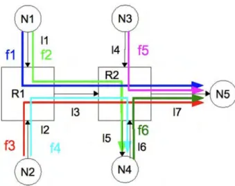
Figure 2. An example of a SpaceWire network (only edges used by at least one flow are displayed)
(4) topology of the network as we will show in the next Section.
The proof of termination of the method and its complexity are given in the Appendix.
IV. EXAMPLES
A. Application of the method of computation
We will now study how the method works on an example of a SpaceWire network. The network is pictured on Figure 2. It contains 5 nodes and 2 SpaceWire routers. Six flows share the network and are represented. We do not need to know the throughput of each flow, only the maximum packet size, which is noted
Ti,
i E{I, ... ,
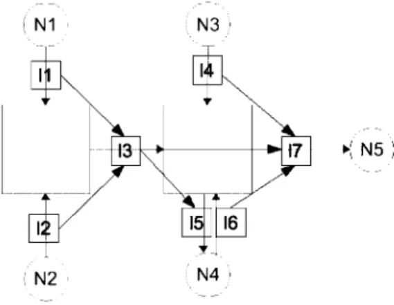
6}.First the dependency graph (see the Appendix for the definition) is computed and it is verified that it is not cyclic. This graph is drawn in Figure 3. It is easy to see that it has no cycle so that the computation can be started safely. We will first compute a bound on the worst-case delay for flow 1 which starts in N1 and ends in N«.
We first have
d(fl' fir st(fl))
==
d(fl' ll)==
d(f2' next(f2' ll))+
d(fl' next(fl' ll))==
d(f2' l3)+
d(fl' l3)The second half becomes
d(fl' l3)
==
max(d(f3' l7), d(f4' ls))+
d(fl' l7)+
2.dsw with d(fl' l7)==
d(fs, null)+
d(f6, null)+
d(fl' null)+
3.dsw 24 Similarly d(f3, l7)==
d(fs, null)+
d(f6, null)+
d(f3' null)+
3.dsw d(f4' ls)==
d(f4' null)+
dswThe first part of (4) develops into
d(f2,l3)
==
max(d(f3,l7), d(f4, ls))+
d(f2, ls)+
2.dswand
Substituting the developments in (4) and using (2) we get: d(f l)
==
T1+
T2+
Ts+
T6 1, 1 C T3+
Ts+
T6 T4+
2.max( C+
2.dsw , C)+
9.dsw (5) Similarly, for f4 we find:d(f l)
==
T3+
T4+
Ts+
T6 4,2 C T1+
Ts+
T6 T2+
2.max( C+
2.dsw , C)+
9.dsw (6) Forfs
we first have:d(fs, l4)
==
d(fs, next(fs, l4))==
d(fs, l7)==
max(d(fl' null), d(f3, null))+
d(f6' null)+
d(fs, null)+
3.dswwhich gives us d(f l)
==
Ts+
T6 S,4 Ct:
T3 (7)+
max( C' C)+
3.dswB. Remarks on the results
Several points can be observed concerning these results. First note that (5) and (6) are similar. (6) can be obtained from (5) by swappingT; and
T3 on the one hand, and T2 and T4 on the other
hand. This is coherent with the fact that Nl and
N2 have identical communication patterns with
N4 and Ns.
We thus see in (5) that
fs
and f6 have a biggerimpact than f2 and f3 on the delay endured by fl.
Therefore, unless T4 is greater than T3
+
Ts+
T6 ,in the worst case, a packet from fl will be delayed
three times by packets from
fs
and f6, twice bypackets from f3 and once by a packet from f2.
Note that this holds true for f4 although it does
not have the same destination as
fs
and f6. This isbecause a packet from f4 can get blocked behind
packets from f3 and [: which may, in tum, be
blocked by packets from
fs
and f6. This examplehighlights the fact that the delays are not caused by an access conflict to a common destination but by the access conflicts to the shared link l3.
N1
N2
N3
---t3--~---~'t-+-I-+---pI
N4
flows starting close to the destination have a large impact on those coming from farther on the network. On the contrary, flows starting far from the destination have a small impact on those closer from the destination.
As a consequence, putting the nodes with the largest sized packets farther from the destina-tion is preferable. This greatly decreases the worst-case delay for the other nodes while only marginally increasing the delay for long packets because only short delays accumulate due to the closer nodes.
However, this only takes into account the worst-case delay, not average delays or through-put. Indeed, when doing a worst-case analysis, we have to assume that, at each link, packets from nodes close to the destination will be interleaved between packets coming from farther away. Of course, this may not happen every time a packet arrives at each link. In this case, sending long packets from nodes far from their destination will end up blocking several links with no bene-fits. Furthermore, this can potentially delay other flows not headed to the same destination but sharing links with the long packets.
c.
Numerical exampleTo better understand the meaning of these formulas, it might be useful to consider a numer-ical example. We will also use this example to illustrate how our method of computation can be used as a tool to make trade-offs on the worst-case delays for the various flows by changing the size of packets.
We will use the following values for the max-imum packet sizes:
Tl ,T3 :5120 B
T2,T4 :50 B
T
s,
T6 :1000 BFigure 3. Dependency graph for the network example (in bold)
Besides, (7) shows that packets from
fs
are delayed only once by a packet from f4 and onceby a packet from fl or f3.
These observations suggest that if several nodes send data to a common destination (a mass memory module for instance) using shared links,
Those are typical values if, for instance, Nl and N2 are observations instruments, N4 is a processor module, Ns is a mass memory module and N3 a monitoring equipment. BothNl and N2 send data at a high rate with large packet sizes to N«. They also send monitoring traffic to N4 which synthesizes it and send it to the memory. The monitoring traffic (f2 and f4) is considered
We use C
==
200 Mbps as the capacity for every link and dsw==
0.5 us as the switchingdelay in both routers. With the same values, we compute both the best- and worst-case delays for
f1, f4 and [e. The best case delay is the delay
when the packet suffers no delays in any router. Results are given in Table I.
Table I
DELAYS FOR THE EXAMPLE OF NETWORK (WITHOUT FRAGMENTATION)
Flow Best Case Worst Case
fl
0.257 ms 1.076 msf4
3.5 JLS 1.076 msf6
50 JLS 356 JLSConcerning these results, as can be expected given their formulas, f1 and f4 have the same
worst-case delay. However, they have very dif-ferent best-case delays. As a consequence, the ratio between the best and worst case delays is far smaller for f1 (4) than for f4 (307). This
highlights the impact of the recursive blockings that leads to long delays even for small packets. For f6, the ratio is only 7 which is coherent with
the fact that flows starting from nodes close to the destination are less influenced by other flows. In order to reduce the worst-case delay for f4,
we can try to fragment the large packets from f1
and f3 in smaller chunks of 256 bytes. As can be
seen in Table II, the worst-case delay for f4 goes
down to 346 us which is roughly one third of the delay without fragmentation. The delay for f5 is
also reduced in the same proportion.
However, the fragmentation has a cost for fl.
As we now need to send 20 fragments to transmit the same information, the worst-case delay for a whole packet becomes 6.9 ms which is almost 7
times more than before.
v.
CONCLUSION AND FUTURE WORKWe have presented a simple method of compu-tation that allows us to compute an upper bound
Table II
DELAYS FOR THE EXAMPLE OF NETWORK (PACKETS FROM
fl
ANDf3
ARE FRAGMENTED)Flow Best Case Worst Case
fl
0.276 ms 6.9 msf4
3.5 JLS 346JLsf6
50 JLS 113 JLS26
on the worst-case end-to-end delay of flows car-ried by a SpaceWire network. This bound is such that it can never be exceeded by a packet as long as the network does not fail. This is especially important for control traffic whose timely delivery is critical to the operation of a satellite. The method uses a recursive definition of the delay endured by each packet in each router to obtain the bound.
Furthermore, the example illustrates the huge difference between the best and worst case delays for a given flow. It also illustrates the fact that the impact of each flow on the delay of other flows varies according to the distance between the source and destination of the flow. Developing the results formally reveals which flows have more impact on others. Finally, we showed on the example how our method can be used as a tool to make trade-offs on the worst-case delays for the various flows in order to better dimension the network.
We have three perspectives to extend our method of computation. The first is to complete the modelisation of SpaceWire by adding Group Adaptative Routing and packet priorities in the model. This will allow us to compute tighter bounds than at present.
At the moment, we do not make strong hypoth-esis on the input traffic. We only suppose that each flow has a maximum packet size. Although this increases the generality of the method, it also means that the results we get may be pessimistic. Thus we plan to use a more precise modelling of the input traffic to obtain tighter bounds. For example, we could use arrival curves to describe the traffic instead of supposing that each flow tries at the maximum speed.
Another interesting direction is to model SpaceWire-RT using the method we have ap-plied for SpaceWire. SpaceWire-RT ([8]) is an extension of SpaceWire, designed as a Quality Of Service layer between a SpaceWire network and its applications. At the moment, it is only a draft but it should provide better temporal guarantees to critical flows. Using our method, we should be able to determine what improvements it will bring for worst-case delays.
ACKNOWLEDGMENT
This work was supported by a PhD grant from the CNES and Thales Alenia Space.
REFERENCES
[1] S. M. Parkes and P. Armbruster, "SpaceWire: A space-craft onboard network for real-time communications,"
IEEE-NPSS Real Time Conference, no. 14, pp. 1-5, Feb
2005.
[2] ECSS, "ECSS-E-ST-50-12C, SpaceWire - links, nodes, routers and networks," pp. 1-129, Aug 2008.
[3] IEEE Computer Society", ''''IEEE Standard for Hetero-geneous Interconnect (hie) (lowcost, low-latency scal-able serial interconnect for parallel system construc-tion)"," IEEE Standard13551995, 1996.
[4] J. T. Draper and J. Ghosh, "A comprehensive analytical model for Wormhole Routing in multicomputer sys-tems," Journal of Parallel and Distributed Computing, pp. 1-34, Jan 1994.
[5] W. Dally, "Performance analysis of k-ary n-cube in-terconnection networks," Computers, IEEE Transactions
on, vol. 39, no. 6, pp. 775 - 785, Jun 1990.
[6] J.-Y. Le Boudec and P. Thiran, "Network Calculus: a theory of deterministic queuing systems for the internet,"
Springer Verlag, no. LNCS 2050, pp. 1-265, Apr 2004.
[7] A. Mifdaoui, F. Frances, and C. Fraboul, "Real-Time characteristics of switched ethernet for "1553b"-embedded applications: Simulation and analysis,"
Indus-trial Embedded Systems, 2007. SIES '07. International Symposium on, pp. 33 - 40, Jun 2007.
[8] S. Parkes and A. F. Florit, "SpaceWire-RT initial proto-col definition v2.1," pp. 1-120, Feb 2009.
[9] W. Dally and C. Seitz, "Deadlock-free message routing in multiprocessor interconnection networks,"
Computers, IEEE Transactions on, vol. C36, no. 5, pp. 547
-553, May 1987.
ApPENDIX A
PROOF OF TERMINATION OF THE METHOD We first define the link dependency graph D for a network represented by the graph Q(N, L)as the directed graph D =
Q(L, E) where the nodes L of D are the links of Q(N, L)
and the edges E are the pairs of links used successively by a flow:
E = {(li,lj) EL [or which
3jE Flnext(j, li) =lj}
Theorem 1: For any flow j in F and any link l in
links(j), the computation of d(j, l) finishes if and only if D is acyclic.
Proof: ::::} Suppose there's a cycle in D. Sincenext(j, l)
cannot return l for any l (a packet cannot use the same
link twice in a row), this cycle's length is at least 2. Given the definition of d, this means we can find a flow j and
a link lsuch that computing d(j, l) requires calling d(j, l)
during the recursion. Thus the computation of d(j,l) does not finish.
<¢::: Suppose D is acyclic. We can then use topological
sorting to assign a total order to the vertices of D such that if
u.,
lj) E E then i. > lj (if D is not connected in the graph theory sense we can order each connected component individually then arbitrarily order the component). From the definition of E and next(j, l), it follows that computingd(j, l) only requires calls to d with links inferior to l as parameters. Since F is a finite set andd(j,l) is called only
once for some givenj andl,it follows that computingd(j, l)
always terminates.
•
Note that as shown in [9] that for an interconnection network using Wormhole Routing under assumptions similar to ours, it is equivalent to say that the link dependency graph is acyclic and that the network is deadlock-free. Since deadlock prone networks would not be valid for satellite use, Theorem 1 shows that the computation finishes in every pertinent case. This is also coherent with the fact that, when the computation does not finish, d(j,l) becomes infinite which is characteristic of a deadlock.
A simple way to check beforehand if the computation will finish is to use the adjacency matrix of the dependency graph and iterate it. If it converges toward the zero matrix then there are no cycles in the graph. However, if a power of the matrix has only 1 on its diagonal, it means that the dependency graph is cyclic and the sum will diverge.
ApPENDIXB
COMPLEXITY OF THE ALGORITHM The exact number of operations required to compute
d(j,l) on a given network will vary with the topology and the number of conflicting flows on each link. However, we can compute an upper-bound on the number of operations without difficulties.
Let us notenthe number of flows in F andm the number of links inL.If we compute naively the delay for each flow, the size of the computation will increase exponentially with the number of flows in conflicts on each link. However, it is easy notice that the number of possible calls tod(j, l) is finite and bounded byn.m. Thus, if we store the results of all the calls during the computation, the complexity of the computation will be O(n.m).