HAL Id: hal-02282919
https://hal.inria.fr/hal-02282919
Submitted on 10 Sep 2019HAL is a multi-disciplinary open access archive for the deposit and dissemination of sci-entific research documents, whether they are pub-lished or not. The documents may come from teaching and research institutions in France or abroad, or from public or private research centers.
L’archive ouverte pluridisciplinaire HAL, est destinée au dépôt et à la diffusion de documents scientifiques de niveau recherche, publiés ou non, émanant des établissements d’enseignement et de recherche français ou étrangers, des laboratoires publics ou privés.
Observer Design for an Inverted Pendulum with Biased
Position Sensors
Stanislav Aranovskiy, Andrei Biryuk, Evgeny V. Nikulchev, Igor Ryadchikov,
Dmitry Sokolov
To cite this version:
Stanislav Aranovskiy, Andrei Biryuk, Evgeny V. Nikulchev, Igor Ryadchikov, Dmitry Sokolov. Ob-server Design for an Inverted Pendulum with Biased Position Sensors. Izvestia Rossiiskoi Akademii Nauk.Teoriya i Systemy Upravleniya / Journal of Computer and Systems Sciences International, MAIK Nauka/Interperiodica, 2019, 58 (2), pp.297-304. �10.1134/S1064230719020023�. �hal-02282919�
РОБОТОТЕХНИКА УДК 681.5.09
OBSERVER DESIGN FOR AN INVERTED PENDULUM WITH BIASED POSITION SENSORS1
S. V. Aranovskiy1,2, A. E. Biryuk3, E. V. Nikulchev4,*, I. V. Ryadchikov3, D. V. Sokolov5
1 France, Cesson-Sévigné, CentraleSupelec-IETR,
2 Russia, Saint Petersburg, ITMO University
3 Krasnodar, Kuban State University
4 Moscow, MIREA– Russian Technological University
5 Nancy, France, Université de Lorraine
*e-mail: nikulchev@mail.ru Initial submission on 28.10.18 г. Revised submission on 09.11.18 г. Accepted for publication on 26.11.18 г.
Inverted pendulums can be considered as an approximation for the stabilization problem for legged robots. In this paper we design a linear observer for a reaction wheel inverted pendulum under biased angle measurements. The reaction wheel is a flywheel that allows the free spinning motor to apply the control torque on the pendulum. In this paper we consider the stabilization problem in the presence of a constant unknown bias in the pendulum angle measurements; this problem has important practical implications, allowing for less precise sensor placement as well as a closer approximation for the control of legged robots. This paper provides a theoretical and experimental basis for the estimation of the velocities and the bias in the system.
Introduction. Walking robotic systems are widely used for moving in difficult conditions
such as overcoming of obstacles, turning in tight areas, moving over rough and/or unknown terrains [1]. Walking robots move by periodically lifting their legs, and, regardless of the number of legs and the gait used [2], the locomotion is characterized by the displacement of the center of mass with respect to the contact points. One of the approaches to modeling and stabilization of walking robots are the inverted pendulums [3, 4]. The center of mass of an inverted pendulum is located above the supporting points, it can be considered as an approximation of the mechanical configuration of bipedal walking robots in the problem of dynamic compensation for the deviation of the robot body from the equilibrium position that occurs when the device is walking.
1 This work is supported by the Ministry of Education and Science of the Russian Federation (GosZadanie grants № 8.2321.2017/ПЧ и 8.8885.2017/8.9).
The analysis of the mathematical models of inverted pendulums and the design of control laws can be done with computational [5, 6] and imitational methods [7, 8] based on the equations of motion. The advantage of the control law design methods that use the differential equations of motion are high accuracy and numerical stability of the resulting solutions [9], ability to analyze the behavior of the system with varying physical parameters. Analytic solutions can also be used for a parametric identification of the system.
In the same time, the computational power of control devices allow to implement fuzzy algorithms and artificial intelligence methods; it allows to use for the control tasks a large variety of methods heavy computational capabilities such as artificial neural networks [10], fuzzy and neuro-fuzzy control systems [11] based on evolutionary computations [12] and other heuristic methods. The disadvantages of these solutions include the dependence on the volume and quality of empirical samples of training data, as well as the inability to quickly compensate for significant variations in the operating conditions, leading to model inconsistencies with real data.
The article covers the problem of stabilization of one-dimensional inverted pendulum equipped with a flywheel, under a systematic error in the position sensor readings. The stabilization is achieved with a LQR-controller. We use a linear observer to correct the bias of the position sensor and to estimate the velocities in the system. The advantages of this observer include the fact that it operates at arbitrary motion trajectories of the inverted pendulum in contrast to the previously proposed solutions operating only at the stationary point [13].
The experiments conducted on the test hardware demonstrate the effectiveness of the selected observer.
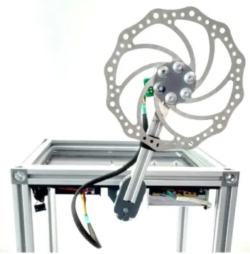
1. Experimental setup and the problem statement. Figure 1 shows an image of an
experimental setup where the controller and the developed observer are tested. The flywheel is actuated by a 70W BLDC motor (Maxon EC 45), which is driven by a controller (Maxon EPOS2 50/5) in torque mode. The motor controller measures the current and the angle of the rotor. STM32F407 microcontroller is used as a main computing unit, interacting with the motor controller over the CANopen protocol. The angle of the pendulum is measured by an optical incremental encoder with a resolution of 2500 pulses per revolution.
Figure 2 shows a schema with notations. The following physical parameters are used to
derive the equations of setup: mp – the mass of the pendulum, mr – mass of the rotor, lp – distance
from the pivot to pendulum’s center of mass, lr – distance from the pivot to the rotor’s center of
mass, Ip – moment of inertia of the pendulum (for rotating about the center of mass), Jr – flywheel’s
moment of inertia, – pendulum angle w.r.t. the vertical, r – angle of the rotror w.r.t the pendulum, – torque applied to the rotor.
Here are the values of the parameters used in our experiments: mp = 0.58 kg, lp = 0.10 m, Jp
= 3.8 10–3 kg m2, m
r = 0.35 kg, lr = 0.22 m, Jr = 12/48 10–4 kg m2. The friction in the pivot is very low and therefore we neglect it.
In order to find the Lagrangian of the system, we write down the expressions for the kinetic and the potential energies of the system. According to the König theorem, the kinetic energy of a pendulum body (without the flywheel) is given as:
2 2
1 ( ) .
2
p p p p
T m l J
Similarly, the kinetic energy of the flywheel has the following expression:
2 2 2 1 1 . 2 ( ) 2 r r r r r T m l J
The potential energy can be written as follows:
( p p r r) cos .
P m l m l g
The Lagrangian can be found as:
.
p r
T T P
+
To simplify the expressions, let us introduce the following notations:
2 2, , ( )/ .
p p p r r p r p p r r
J J m l m l m m m l m l m l m
Then the Lagrangian can be written as:
2 2 1 1 cos . 2J 2Jr( r ) mlg + .
For convenience, all partial derivatives are written out:
( ), 0, r r r r J + + (J Jr) Jr r, mlgsin . + +
Recall that the Lagrange equations have the following form:
, i i i d dt q q + +
where qi – is generalized coordinate, i – the corresponding generalized force. In our case q1 = r, q2
= , so the equations of motion have the following expression:
, ( ) sin 0, r r r r r r J J J J J mlg
where – is the torque applied by the motor.
Converting the equations to the normal form, i.e., solving the equations for the higher derivatives yields: sin , sin . r r r mlg J J JJ J mlg J J (1.1)
Our goal is to implement a control law (and develop necessary observers) to achieve the stabilization of the system (1.1) under the systematic bias present in the position sensors.
2. The design of a linear control law. We suppose that the motor controller compensates
the back-EMF and allows us to use torque as a direct input. Then in our model (1.1) we suppose =
kI, where the current I is our input signal.
The linearized system takes the following form:
, X AX BI (2.1)
Where, neglecting the friction, we have:
0 1 0 0 , 0 0 , . ( ) 0 0 r r r mlg k X A B J J mlg J J k J J J
We are looking for a linear control law I = –KX, where K = (k1, k2, k3). The vector K is
chosen to minimize the following quality criterion:
T T 0 ( ) , F X QX I RI dt
It can be done with aid of Linear Quadratic Regulator (LQR) method [14]. The matrices Q and R are 3 3 and 1 1; they are design parameters. For our system we have found the following vector of gains:
( 378, 55, 1)
K
Once we have determined K, the system (3.1) under control law I = –KX takes the following expression: X = (A – BK)X. LQR guarantees that real parts of the eigenvalues of the matrix A – BK are negative.
3. Effect of the position sensor calibration error. In case of imperfect calibration of the
pendulum angle sensor, the sensor reading may have some constant bias . In this case our system
receives incorrect input signal I = –KX – K( 0 0)T. Therefore, system (2.1) can be rewritten as
follows:
Τ
( ) ( 0 0) .
X A BK X BK
Let us find the stationary point of the system:
Τ Τ 1 Τ 1 3 0 ( ) ( 0 0) ( ) ( 0 0) 0 0 . A BK X BK k X A BK BK k .
Since all eigenvalues of the matrix (A – BK) have a negative real part, the stationary point we have found is globally asymptotically stable. It means that under biased angle measurements the
pendulum stabilizes at the true zero position, however the reaction wheel reaches a steady non-zero angular velocity, proportional to the calibration error.
4. Observer design. In our experimental setup we can directly measure the pendulum’s
angle, however we do not dispose of angular speed sensors. Our linear control law requires the speed measurements. Moreover, the control quality deteriorates if the sensors are not correctly calibrated. In this work we consider the case when the angle measurements have constant unknown bias . In other words, insteand of true readings θ the sensors reads + .
Therefore, our goal is to design an observer that will allow us to determine true angle , angular speed and the bias with a precision sufficient for the stabilization task. As it was shown in the section 3, the bias can be estimated once the pendulum is already stabilized, however, we want to be able to estimate it along arbitrary trajectories of the system, thus reducing transient time while avoiding self-oscillations.
To achieve our goal, we use the fact that the control action is known for all past time intervals. We will construct an auxiliary system of differential equations, whose solutions converge asymptotically to the unknown values. In other words, the output of our observer gives the system state in the phase space.
We know the current I as a function of time, therefore we know the torque = kI, and can analyse both equations of the system (1.1) independently one from another:
sin mlg kI x J J (4.1)
Let us denote the angle measurements as y = + (recall that denotes the true position) and introduce following notations:
ˆ , ˆ , ˆ x x
where x – is the system state vector, and ˆx– the vector with our estimations (output of our the
observer). We also denote the estimation error as x = ˆx – x. Let us add to (4.1) one more equation
= 0 and rewrite the system in the matrix notations using x coordinates (x1 = , x2 = , x2 = ): 2 1 sin , , 0 x x a x bI y Cx (4.2)
where a = mlg/J, b = –k/J, C = [1 0 1]. In these settings we have following equalities:
1 3 ˆ3 3.
x y x y x x
We suppose that the calibration error is small, therefore the following approximation holds:
1 3 3 3 3 3
sin( )x sin(y xˆ x)sin(y xˆ)cos(y x xˆ ).
Then the observer for ˆxcan be written in the following form:
2 1 3 2 3 ˆ sin( ) , , 0 ˆ ˆ ˆ ˆ x l x a y x bI l y y Cx l (4.3)
where y = ˆy – y =Cx, and the gain vector L = [l1 l2 l3]T will be defined later on. By subtracting
(4.2) from (4.3), we obtain an equation for the estimation error dynamics:
3 0 1 0 ˆ 0 0 cos( ˆ) . 0 0 0 x x x a y x x LCx (4.4)
This is a time-varying linear system of differential equations for the vector x. In points cos(y – ˆx )3
= 0 it becomes singular and thus non-observable. Let us denote z = y – ˆx ,3
0 1 0 ( ) 0 0 cos( ) . 0 0 0 A z a z
Then the equations (4.4) take the following form:
( ( ) ) . x A z LC x
Let us verify the stability of the system for all z. By writing down the characteristic polynomials of the matrix A(z) – LC for the cases cos(y1 – ˆx ) = 1: 3
3 2
1 3 2 3
( ) ,
s l l s l s al
we can see that there is no such constant vector L = [l1 l2 l3]T, such that the matrix A(z) – LC
satisfies the Hurwitz condition for both cos(y1 – ˆx ) = 1 and cos(y3 1 – ˆx ) = –1. In other words, an3
observer with constant gain values would not function along all trajectories where the pendulum crosses the horizontal position.
For our observer let us suppose that the initial position and all the trajectory of the pendulum lie in the upper semi-circle, i.e. we have |z| 0, где /2 > 0 > 0. This supposition is fair, since for
the stabilization problem the pendulum will be close to the vertical; moreover, deviations for over /2 invalidate the linearized model. Let us also suppose that the signal y also satisfies our upper semi-circle hypothesis. This supposition is also reasonable, since typical calibration errors are very small, allowing us to formulate bounds on the signal z.
With above suppositions the observer design can be formulated as a linear matrix inequalities problem: T 0, P P . T (A(0) LC P) P A( (0) LC)0,.
Indeed, if it is possible to find L, such that the above system has feasible solutions, then the matrix P serve as a weight matrix for a quadratic Lyapunov function for the estimation error. The time derivative of the Lyapunov function is negative for all values of z, it follows from the second and third inequalities.
For our pendulum we chose the following solution of the linear matrix inequalities:
Τ
[546 1100 508] ,
L
this solution yields the 0.5 seconds transient time.
5. Experiment. We performed two experiments with the hardware shown in Figure 1. In
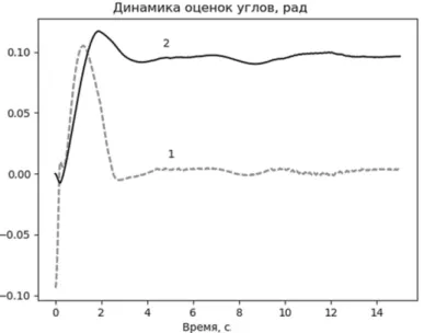
both experiments the bias was set manually to = 0.1 radian. The first experiment shows the behavior of the system without bias estimation, and the second uses the observer we have built. The results are shown in Figures 3–5.
On one hand, as it is shown in Figure 3, the pendulum is stabilized in both experiments. On the other hand, Figure 4 shows that the angular velocity of the flywheel reaches zero, whereas without bias estimation the flywheel velocity stabilizes at 170 rad/s, thus confirming our calculations.
Figure 5 shows the dynamics of the observer (in the second experiment). The bias estimation converges to the preset value = 0.1 and the angle estimation converges to zero.
Both experiments confirm our calculations; we have successfully tested the observer for a bipedal robot [15].
Conclusion. In this paper we have presented a design of a linear observer for the
stabilization of a reaction-wheel inverted pendulum in presence of some constant unknown bias in the angle measurements. This problem has important practical implications, enabling for a dynamic calibration error corrections. The observer we have built works for arbitrary trajectories of the system, whereas state of the art approaches [13] work only for the upper equilibrium point. Our approach, coupled with a linear control law, does not induce self-oscillations, and it was verified theoretically and validated experimentally. We have also reduced the cost of the hardware by replacing the angular speed sensors, with corresponding soft sensors.
1. Брискин Е.С., Калинин Я.В., Малолетов А.В., Шурыгин В.А. Об оценке эффективности шагающих роботов на основе многокритериальной оптимизации их параметров и алгоритмов движения // Изв. РАН. ТиСУ. 2017. № 2. С. 168–176. 2. Савин С.И., Ворочаева Л.Ю. Методы управления движением шагающих внутритрубных роботов // Cloud of Science. 2018. Т. 5. № 1. 163–195. 3. Гришин А.А. Ленский А.В., Охоцимский Д.Е., Панин Д.А., Формальский А.М. О синтезе управления неустойчивым объектом. Перевернутый маятник // Изв. РАН. ТиСУ. 2002. № 5. С. 14–24. 4. Решмин C.А., Черноусько Ф.Л. Оптимальное по быстродействию управление перевернутым маятником в форме синтеза // Изв. РАН. ТиСУ. 2006. № 3. С. 51–62. 5. Franco E., Astolfi A., Baena F.R. Robust Balancing Control of Flexible Inverted-Pendulum
Systems // Mechanism and Machine Theory. 2018. V. 130. P. 539–551.
6. Hua Y., Yang Z. Simple Rotary Inverted Pendulum and the Control Device // Applied Mechanics & Materials. 2016. V. 851. P. 445–448.
7. Chen X., Yu R., Huang K., Zhen S., Sun H., Shao K. Linear Motor Driven Double Inverted Pendulum: A Novel Mechanical Design as a Testbed for Control Algorithms // Simulation Modelling Practice and Theory. 2018. V. 81. P. 31–50.
8. Sánchez J., Dormido S., Pastor R., Morilla F. A Java/MATLAB-based Environment for Remote Control System Laboratories: Illustrated with an Inverted Pendulum // IEEE Transactions on Education. 2004. V. 47. № 3. P. 321–329.
9. Chatterjee S., Das S.K. An Analytical Formula for Optimal Tuning of the State Feedback Controller Gains for the Cart-Inverted Pendulum System // IFAC-PapersOnLine. 2018. V. 51. № 1. P. 668–672.
10. Rubio J. J. Discrete Time Control Based in Neural Networks for Pendulums // Applied Soft Computing. 2018. V. 68. З. 821–832.
11. Bellino A., Fasana A., Gandino E., Garibaldi L., Marchesiello S. A time-varying inertia pendulum: Analytical modelling and experimental identification // Mechanical Systems and Signal Processing. 2014. V. 47. № 1–2. P. 120–138.
12. Ping Z., Huang J. Approximate Output Regulation of Spherical Inverted Pendulum by Neural Network Control // Neurocomputing. 2012. V. 85. P. 38–44.
13. Gajamohan M., Merz M., Thommen I., D'Andrea, R. The Сubli: A Cube That Can Jump up and Balance // 2012 IEEE/RSJ Intern. Conf. on Intelligent Robots and Systems (IROS). Piscataway: IEEE Publ., 2012. P. 3722–3727.
14. Anderson B.D.O., Moore J.B. Optimal Control: Linear Quadratic Methods. Mineola: Dover Publ. Inc., 2007.
15. Ryadchikov I., Sechenev S., Nikulchev E., Drobotenko M., Svidlov A., Volkodav P., Vishnykov R. Control and Stability Evaluation of the Bipedal Walking Robot Anywalker // International Review of Automatic Control. 2018. V. 11. №. 4. P. 160–165.
Figure 1. Inverted pendulum hardware
Figure 3. The angle of the pendulum in two experiments: 1 – without bias estimation, 2 – the
experiment with bias estimation
Figure 4. The flywheel speed in two experiments: 1 – without bias estimation, 2 – with bias