Analysis of two methods of poles extraction for antenna caracterization

HAL Id: hal-01409203

https://hal.archives-ouvertes.fr/hal-01409203

Submitted on 5 Dec 2016

HAL is a multi-disciplinary open access

archive for the deposit and dissemination of

sci-entific research documents, whether they are

pub-lished or not. The documents may come from

teaching and research institutions in France or

abroad, or from public or private research centers.

L’archive ouverte pluridisciplinaire HAL, est

destinée au dépôt et à la diffusion de documents

scientifiques de niveau recherche, publiés ou non,

émanant des établissements d’enseignement et de

recherche français ou étrangers, des laboratoires

publics ou privés.

Analysis of two methods of poles extraction for antenna

caracterization

François Sarrazin, A Sharaiha, P Pouliguen, P Potier, J Chauveau

To cite this version:

François Sarrazin, A Sharaiha, P Pouliguen, P Potier, J Chauveau. Analysis of two methods of poles

extraction for antenna caracterization. IEEE International Symposium on Antennas and Propagation

(APSURSI 2012), Jul 2012, Chicago, IL, United States. �10.1109/APS.2012.6348637�. �hal-01409203�

Analysis of Two Methods of Poles Extraction for

Antenna Caracterization

F. Sarrazin, A. Sharaiha

francois.sarrazin@univ-rennes1.fr

P. Pouliguen, P. Potier, J. Chauveau

France

philippe.pouliguen@dga.defense.gouv.fr

Abstract— Antenna radiation characteristics can be modeled by some poles and residues. In this paper, we compare two different methods to extract these poles of a noisy antenna radiation in frequency and in time domain: the Cauchy method and the Total Least Square Matrix Pencil Method respectively. Results are presented for a dipole antenna and an Archimedean spiral antenna.

I. INTRODUCTION

Since many years, the Singularity Expansion Method (SEM) [1], introduced by C. E. Baum in 1971, is studied to be applied to target identification. In fact, SEM represents a solution of an electromagnetic problem in terms of singularities (poles). Since singularities are independent of the direction of the incoming wave, it makes it useful for scatter identification. More recently, this method has been applied in both time and frequency domains to model antenna effective length, in order to fully describe the antenna pattern, directivity and gain using only a few set of parameters (poles and residues) [2] [3]. They are extracted using different methods. In frequency domain, we can use the Cauchy method. In time domain, the most popular one is the Matrix Pencil Method (MPM). The purpose of this paper is to compare these methods applied on antenna radiation responses and to analyze their robustness to Signal-to-Noise Ratio (SNR), which to the author’s knowledge has never been done. In section II, we recall both methods. In section III, we compare these methods applied on dipole and Archimedean spiral antenna responses in presence of noise.

II. SEMTHEORY

A. Total Least Square Matrix Pencil Method (TLS-MPM)

In time domain, Hua and Sarkar [4] propose to model the noisy data set 𝑦𝑘 as

𝑦𝑘 ≈ 𝑁𝑛=1𝑅𝑛𝑒𝑠𝑛𝑘 = 𝑁𝑛=1𝑅𝑛𝑧𝑛𝑘 

where 𝑁 is the number of poles, 𝑘 = 0,1, … , 𝐾 − 1, 𝐾 is the number of sampled data (𝐾 > 2𝑁), 𝑅𝑛 the residues, 𝑠𝑛 the

poles (𝑠𝑛 = 𝜎𝑛± 𝑗𝜔𝑛 with 𝜎𝑛 the damping coefficient and 𝜔𝑛

the resonant pulsation). A data matrix [𝑌] is built (2) in compliance with the pencil parameter 𝐿 , useful in reducing noise in the data and generally chosen between 𝐾/3 and 𝐾/2. Then, a Singular Value Decomposition is carried out as 𝑌 = 𝑈 𝑉 𝐻_{, 𝐻 being the Hermitian transpose, 𝑈 and}

𝑉 are unitary matrices composed of the eigenvectors of

[𝑌][𝑌]𝐻 _{and [𝑌]}𝐻_{[𝑌], respectively. is a diagonal matrix}

containing the singular values of [𝑌].

𝑌 = 𝑦0 𝑦1 … 𝑦𝐿 𝑦1 𝑦2 … 𝑦𝐿+1 ⋮ ⋮ ⋱ ⋮ 𝑦𝐾−𝐿−1 𝑦𝐾−𝐿 … 𝑦𝐾−1 

A significant parameter 𝑀 is now chosen such that the singular values in beyond M are “small” and can be approximated by zero. A reduced matrix [𝑉’] can now be constructed using only the rows corresponding to the 𝑀 most significant value as 𝑉′ = 𝑣1 𝑣2 ⋯ 𝑣𝑀 𝑇 . Next, we define two submatrices [V1’] and [V2’] from [V’] by deleting the last column of [V’] and the first column of [V’], respectively. The problem is reduced to a left-hand eigenvalue problem given by (3). The eigenvalues λ correspond to poles of the system in terms of 𝑧𝑘_.

𝑉2′ = λ 𝑉1′ → 𝑉2′ 𝑉′1 𝐻= λ 𝑉1′ [𝑉1′]𝐻 

B. Cauchy Method

Another method is the Cauchy method [5]. It is applied on a transfer function in frequency domain. The transfer function H(s) is approximated by a ratio of two polynomials as

𝐻 𝑠 = 𝑃𝑀 𝑠 𝑄𝑁 𝑠 = 𝑎𝑚𝑠𝑚 𝑀 𝑛 =0 1+ 𝑁𝑛 =1𝑏𝑛𝑠𝑛 

where 𝑁 = 𝑀 + 1 is the filter order. Equation (4) can also be written as a matrix equation 𝐴𝑥 = 𝑏 with 𝑥 = 𝑏1 ⋯ 𝑏𝑁 −𝑎0 ⋯ −𝑎𝑀 𝑇which is solved using a

least square approach as 𝑥 = (𝐴𝐻_𝐴)−1_𝐴𝐻_{𝑏 . The transfer}

function 𝐻(𝑠) can now be modeled as 𝐻(𝑠) = 𝑅𝑛

𝑠−𝑠_𝑛 𝑁

𝑛=1 

III. APPLICATION ON NOISY ANTENNA RESPONSES

A. Dipole Antenna

To compare the robustness of the methods, we first consider a dipole antenna. Its length is L = 33.75 mm, its radius is R = 0.56 mm and its gap is G = 0.56 mm. It is simulated in frequency domain using HFSS [6] between 1 and 18 GHz with

δf = 17 MHz. The noiseless E-farfield radiated by the dipole antenna in the boresight direction is presented Fig. 1. Cauchy is now applied on this response. An Inverse Fast Fourier Transform (IFFT) is also performed and MPM is applied on the transient response obtained. Poles extracted using both methods are presented Fig. 2. We note that poles are very close and they correspond to the two resonances of the dipole radiation (at λ/2 and 3λ/2). Only the damping coefficient of the second pole (at 12.2 GHz) differs from only 0.2 109 rad/s. Next, we compare these methods in presence of Gaussian white noise added to obtain different Signal to Noise Ratio (SNR) from -10 to 70 dB. For each SNR, ten different sets of noisy data have been used. The number of poles extracted by each method is presented in Table I. A pole is considered well extracted when the resonant frequency is the same than without noise within 5%. When SNR = 10 dB, MPM still extracts the four poles of the response while Cauchy extracts only two poles.

Figure 1. Noiseless E-field of the dipole antenna.

Figure 2. Poles extracted without noise. TABLE I. NUMBER OF POLES EXTRACTED VERSUS SNR.

Method SNR (dB)

-10 0 10 20 30 40 50 60 70

Cauchy 0 0 2 4 4 4 4 4 4 MPM 0 2 4 4 4 4 4 4 4

B. Archimedean Spiral Antenna

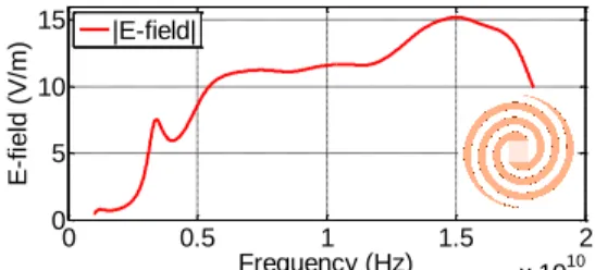
We now consider a one and a half tour UWB Archimedean spiral antenna which radius is 13 mm and is matched between 4.5 and 18 GHz. It is simulated using HFSS between 1 and 18 GHz with δf = 17 MHz. Fig. 3 presents the noiseless E-farfield in the boresight direction. As for the dipole, Cauchy is applied on this response and MPM is applied on its IFFT. Results are presented in Fig. 4. We observe that the first pole (at 3.4 GHz) is well extracted by both methods. For the other poles, resonant frequencies are almost the same but damping coefficients differ. We add a Gaussian white noise to the response and apply both methods. Results are presented in Table 2. When SNR becomes low, MPM still extracts some poles while Cauchy doesn’t.

Figure 3. Noiseless E-field of the Archimedeam antenna.

Figure 4. Poles extracted without noise. TABLE 2. NUMBER OF POLES EXTRACTED VERSUS SNR.

Method SNR (dB)

-10 0 10 20 30 40 50 60 70

Cauchy 0 2 4 6 6 6 6 8 10 MPM 2 4 4 4 6 6 8 12 12

IV. CONCLUSION AND PERSPECTIVES

To our knowledge, these results are the first comparison between MPM and Cauchy method to analyze antenna radiated responses. In both cases, MPM extracts more poles than Cauchy method when SNR becomes low. Moreover, according to the response, the order of the filter must be modified to help the Cauchy algorithm to converge. MPM doesn’t need any modification and is more computational. Additional analyses are in progress to confirm these first interesting results, for example by filtering the early time of radiation responses.

ACKNOWLEDGEMENT

This work was financially supported by the DGA. REFERENCES

[1] C. E. Baum, “On the singularity expansion method for the solution of electromagnetic interaction problems”, EMP Interaction Note 8, Air Force Weapons Laboratory, Kirkland AFB, New Mexico, Dec. 1971. [2] S. Licul and W. A. Davis, “Unified frequency and time-domain antenna

modeling and characterization”, IEEE Transactions on Antenna and

Propagation, vol. 53, No 9, pp. 2882–2888, Sep. 2005.

[3] C. Marchais, B. Uguen, A. Sharaiha, G. L. Ray and L. Le Coq, “Compact characterisation of ultra wideband antenna responses from frequency measurements“, IET, Microwaves, Antennas & Propagation, vol. 5 , Issue: 6, pp. 671-675, 2011.

[4] Y. Hua and T. K. Sarkar, “Matrix pencil method for estimating parameters of exponentially damped/undamped sinusoids in noise”,

IEEE transactions on Acoustics, speech and signal processing, vol. 38,

No , pp. 814-824, May. 1990.

[5] A. L. Cauchy, “Sur la formule de Lagrange relative à l’interpolation”, Analyse Algèbrique, Paris, 1821.

[6] Ansys HFSS, Available: http://www.ansoft.com/products/hf/hfss/.

0 0.5 1 1.5 2 x 1010 0 5 10 Frequency (Hz) E -f ie ld ( V /m ) |E-field| -9 -8 -7 -6 -5 -4 x 109 0 5 10 15x 10 9

Damping Coefficient (rad/s)

F re q u e n c y ( H z ) _{Matrix Pencil} Cauchy 0 0.5 1 1.5 2 x 1010 0 5 10 15 Frequency (Hz) E -f ie ld ( V /m ) |E-field| -10 -8 -6 -4 -2 0 x 109 0 1 2x 10 10

Damping Coefficient (rad/s)

F re q u e n c y ( H z ) _{Matrix Pencil} Cauchy