Faculté des Sciences, 4 Avenue Ibn Battouta B.P. 1014 RP, Rabat – Maroc Tel +212 (0) 37 77 18 34/35/38, Fax : +212 (0) 37 77 42 61, http://www.fsr.ac.ma
Essannouni Fedwa
Discipline : Sciences de l’ingénieur
Spécialité : Informatique et Télécommunications
Titre : Estimation de mouvement robuste et de faible complexité dans les
séquences vidéo.
Soutenue le 10 Septembre 2007
Devant le jury
Président :
D. ABOUTAJDINE professeur à la Faculté des Sciences de Rabat
Examinateurs :
R. OULAD HAJ THAMI professeur à l’ENSIAS, Rabat
A. SALAM Professeur à l’Université du Littoral Côte d'Opale, Calais, France
R. BENSLIMANE Professeur à l’Université Sidi Mohamed Ben Abdellah, Fès
E. MOUADDIB professeur à l’Université de Picardie Jules Verne, Amiens, France
M. ABBAD professeur à la Faculté des Sciences de Rabat
J’adresse mon profond respect et ma profonde gratitude `a Monsieur le professeur Driss ABOUTAJDINE, pour m’avoir accueillie dans son laboratoire, superviser mes travaux de th`ese, et accepter de pr´esider ce jury. Je tiens `a lui exprimer ma reconnaissance pour sa grande disponibilit´e, sa rigueur scientifique, son enthousiasme et ses pr´ecieux conseils qui ont fait progresser ce travail. Qu’il soit assur´e de toute mon estime et de mon profond respect.
Je remercie vivement Monsieur Rachid OULAD HAJ THAMI professeur `a L’ENSIAS d’avoir accept´e d’encadrer et diriger mes travaux de recherche. Les remerciements ex-prim´es ici ne seront jamais `a la hauteur de son implication dans ce travail. Qu’il trouve ici toute ma reconnaissance pour son aide, ses nombreux conseils, son soutien sans faille, sa disponibilit ´e et son dynamisme.
J’exprime mes profonds remerciements `a mon directeur de th`ese, le professeur Ahmed SALAM de l’Universit´e Littoral Cˆote d’Opale de Calais pour l’aide comp´etente qu’il m’a apport´ee, pour sa patience et son encouragement. Ses conseils et ses commentaires m’ont ´et´e fort utiles.
Je remercie tous particuli`erement Monsieur Rachid BENSLIMANE professeur `a l’Universit´e Sidi Mohamed Ben Abdellah de F`es et Monsieur El Mustapha MOUADDIB professeur `a l’Universit´e de Picardie Jules Verne d’Amiens, d’avoir accept´e de juger ce tra-vail et d’en ˆetre les rapporteurs. Je les remercie pour leurs conseils et leurs suggestions qui ont permis l’am´elioration de ce manuscrit. Qu’ils acceptent mes plus vifs remerciements pour leur pr´esence dans ce jury.
ABBAD, professeur `a la Facult´e des Sciences de Rabat et Monsieur le professeur Mo-hammed NAJIM professeur `a l’ENSEIRB de Bordeaux pour leur participation au jury de cette th`ese.
Je veux adresser tous mes remerciements `a Monsieur Radouane FAIZI professeur `a L’ENSIAS, qu’il trouve ici l’expression de ma profonde gratitude et ma reconnaissance pour le temps pass´e `a corriger l’anglais de ma th`ese. Je le remercie pour sa disponibilit´e et sa bonne humeur.
Merci aussi `a tous mes coll`egues dans les laboratoires LRIT GSCM et SI2M. Je leur exprime ma profonde sympathie et leur souhaite beaucoup de bien.
Au cours de la pr´eparation de ma th`ese, j’ai b´en´efici´e d’une bourse d’excellence oc-troy´ee par le CNRST dans le cadre du programme de bourses de recherche du Minist`ere de l’Education Nationale, de l’Enseignement Sup´erieur, de la Formation des Cadres et de la Recherche Scientifique.
defined as searching the best motion vector of the current block in the current frame in a predefined search area in the reference frame.
Among the various approaches for motion estimation, block matching algorithm (BMA) is the most popular. It has been adopted by such leading video compression standards MPEG 1/2/4 and H261/263/264. In a standard BMA, each frame is divided into non overlapping blocks. To exploit the video temporal redundancy, each block in the current frame is compared to all candidate blocks in a search area of a reference frame. The can-didate block that is best matched with the current block, in terms of some block matching distortion measures, such as the sum of absolute differences (SAD) or sum square differ-ences (SSD), is selected as the reference block for compression.
Full search in the block matching algorithm (BMA) finds the global minimum value of matching error surface. It is popular in many applications of video and image processing due its simplicity and easy hardware implementation. However, its overhead computa-tional load for a large search range can be a significant problem in real time applications. Over the past few decades, many fast algorithms to reduce the computation of the full search have been studied using either sum square difference (SSD) or sum absolute differ-ence (SAD). They can be classified into two groups, the lossy and the lossless fast motion estimation methods. The lossy algorithms have some degradation of predicted images when compared with the FS algorithm, whereas the lossless motion estimation gives no degradation of predicted compared images.
A comprehensive survey of block matching techniques is presented in this thesis. The recent and most efficient block matching algorithms are outlined. Based on the insights
gained from the examination and comparison of these block matching algorithms, an improved version of the adaptive rood pattern search algorithm is proposed. It makes use of the propriety of the temporal redundancy of motion vectors. The rest of this work deals with solving the overwhelming complexity of the full search using the fast Fourier Transform. Many metrics are used, namely the sum square difference, the sum absolute difference, the L4 norm and the Andrew’s wave M estimator. The proposed approaches are fast, exhaustive and have a deterministic execution time. They are well suited for real time applications and they benefit from the huge work that has been done in the frequency domain aimed at speeding up the discrete Fourier transform.
approches d’estimation de mouvement, l’algorithme par appariement de blocs (BMA) est le plus utilis´e. Il a ´et´e adopt´e par plusieurs codeurs vid´eo tels que : MPEG 1/2/4 et H261/263/264.
Dans un BMA typique, chaque image est divis´ee en des blocs non-recouverts. Pour exploiter la redondance temporelle de la vid´eo, chaque bloc dans la trame courante est compar´e avec tous les blocs candidats dans une fenˆetre de recherche dans la trame de r´ef´erence. Ainsi, le bloc candidat qui est le plus semblable au bloc courant, en termes d’une certaine mesure de distorsion, telle que la somme des diff´erences absolues (SAD) ou la somme des diff´erences carr´ees (SSD), est s´electionn´e.
La recherche exhaustive (FS) dans l’algorithme par appariement de bloc (BMA) per-met de trouver le vecteur optimal qui minimise la fonction d’erreur utilis´ee dans une fenˆetre de recherche donn´ee. Elle est exploit´ee dans plusieurs applications de traitement de la vid´eo et de l’image en raison de sa simplicit´e et son efficacit´e. Cependant, son temps de calcul ´enorme pour une dynamique de recherche large pr´esente un probl`eme significatif pour des applications en temps r´eel.
Pendant ces derni`eres d´ecennies, plusieurs algorithmes rapides d’estimation de mou-vement ont ´et´e ´etudi´es pour r´eduire le temps de calcul d’une recherche exhaustive (FS) en utilisant soit la somme des diff´erences carr´ees (SSD) ou la somme des diff´erences absolues (SAD). Ils peuvent ˆetre classifi´es en deux groupes principaux, les m´ethodes optimales et les m´ethodes sous optimales d’estimation de mouvement. L’estimation de mouvement avec les m´ethodes sous optimales d´egradent les images pr´edites compar´ees `a celles obtenues avec l’algorithme conventionnel FS. Tandis que l’estimation de mouvement avec les m´ethodes
optimales permettent d’obtenir la mˆeme qualit´e de pr´ediction qu’un algorithme FS. Dans ce m´emoire les techniques d’appariement des blocs les plus r´ecents et efficaces dans la litt´erature sont compar´ees et nouvelles approches sont propos´ees. La majorit´e des algorithmes introduits dans ce travail, contrairement `a plusieurs solutions existantes, ne sont pas bas´es sur le domaine spatial, ils utilisent plutˆot le domaine fr´equentiel. Les approches propos´ees permettent d’acc´el´erer la comparaison entre les blocs en utilisant des m´etriques robustes et non robustes. Elles permettent d’offrir un temps de calcul d´eterministe et rapide tout en gardant une estimation de mouvement ´equivalente `a une recherche exhaustive. L’avantage de ces algorithmes bas´es sur la corr´elation est le champ r´egulier des donn´ees, contrairement `a d’autres algorithmes rapides d’estimation de mou-vement.
List of Acronyms xi
List of Figures xiii
List of Tables xv
1 Introduction 1
1.1 Statement of the problem . . . 1
1.2 Investigated approach and thesis organization . . . 4
2 Block matching algorithms 7 2.1 Introduction . . . 7
2.2 Full search block matching algorithm . . . 8
2.3 Fast full search block matching algorithms . . . 10
2.3.1 Successive elimination algorithm (SEA ) . . . 10
2.3.2 Multilevel successive elimination algorithm (MSEA) . . . 11
2.3.3 Predictive fine granularity successive elimination (FGSE) . . . 12
2.3.4 Normalized PDS (NPDS) algorithm . . . 15
2.4 Fast Block matching algorithms . . . 17
2.4.1 Diamond Search (DS) . . . 17
2.4.2 Hexagonal Search (HEXBS) . . . 19
2.4.3 Adaptive Rood Pattern Search (ARPS) . . . 19
2.4.4 Adaptive irregular pattern search (AIPS) . . . 21
2.5 Proposed algorithm (DMPS) . . . 22
2.5.1 Overview . . . 22
2.5.2 Initial region search . . . 23
2.5.3 Early search judgement . . . 24
2.5.4 Refined search . . . 25
2.6 Simulations . . . 26
2.7 Conclusion . . . 27
3 Exhaustive SSD matching using frequency domain 29 3.1 Introduction . . . 29
3.2 Fourier and correlation based methods . . . 31
3.2.1 Translational motion in the Fourier domain . . . 31
3.2.2 Correlation based methods . . . 32
3.2.3 Frequency components . . . 35
3.3 The proposed algorithms . . . 37
3.3.1 Mathematical background: . . . 37
3.3.2 The proposed correlation methods . . . 40
3.3.3 Computational complexity . . . 42
3.4 Simulation results . . . 46
3.5 Conclusion . . . 49
4 Exhaustive SAD matching using frequency domain 53 4.1 Introduction . . . 53
4.2 The proposed SAD approximation . . . 55
4.2.1 Problem formulation . . . 55
4.4 Conclusion . . . 66
5 Robust matching algorithms 67 5.1 Introduction . . . 67
5.2 Fast frequency template matching based on Lp norms . . . 69
5.2.1 The proposed L4 correlation . . . 70
5.3 The proposed Andrew’s correlation . . . 73
5.3.1 Andrew’s M estimator criteria . . . 73
5.3.2 Fast robust correlation . . . 74
5.3.3 The proposed Andrew’s correlation (AC) . . . 75
5.4 Simulation results . . . 77
5.4.1 Comparative performance assessment . . . 78
5.4.2 Comparison between the proposed method and the FSBMA in the presence of outliers . . . 78
5.5 Conclusion . . . 78
6 Conclusion 83 6.1 Possible extensions . . . 84
List of Acronyms
HVS Human Visual System.
BMA Block matching algorithm.
SAD Sum of absolute differences.
SSD Sum square difference.
MV Motion vector.
FS Full search.
TSS Three Step Search.
NTSS New Three Step Search.
SES Simple and Efficient TSS.
4SS Four Step Search.
DS Diamond Search.
ARPS Adaptive Rood Pattern Search.
SEA Successive elimination algorithm.
MSEA Multilevel successive elimination algorithm.
FGSE Predictive fine granularity successive elimination.
HEXBS Hexagonal search .
ZMP Zero-motion prejudgment.
AIPS Adaptive irregular pattern search.
SP Searching point.
FFT Fast Fourier Transform .
CORR Classical cross correlation.
PC Phase correlation method.
OC Orientation correlation method.
FRcorr Fast robust correlation.
MSE Mean square error.
MAD Mean absolute difference.
flops Floating-point operations.
List of Figures
1.1 An example of successive frames in video sequences. . . 2
2.1 Search area in block matching algorithm. . . 9
2.2 Partition process in the MSEA algorithm. . . 12
2.3 Partition process in the FGSE algorithm where there are 86 levels in total in contrast with only five levels (level 0, level 1, level 5, level 21, and level 85) in MSEA. . . 14
2.4 The group of pixel locations for the calculation of the partial distortion dp(x, y). sp, tp are the offsets of the upper left corner point of the partial block. . . 15
2.5 Spiral scanning path of NPDS. . . 16
2.6 LDSP and SDSP patterns. . . 17
2.7 Diamond Search. . . 18
2.8 Hexagonal search. . . 19
2.9 Initial region search in ARPS algorithm. . . 20
2.10 Adaptive irregular pattern search. . . 21
2.11 Example of search pattern of DMPS. . . 23
2.12 Refined search pattern. . . 25
3.1 Reconstructed frame from Carphone cif sequence using different correlation methods for block size 162 and corresponding search range of ±8. . . . 32
4.1 Absolute kernel |x| approximation using Fourier Cosine Series. . . . 55
4.2 Square error between the absolute kernel f (x) = |x| and its approximation
fL(x) using different levels L. . . . 56
4.3 A simple flow chart for the proposed frequency SAD matching algorithm. . 59
4.4 Improvement in arithmetic complexity by using the proposed frequency method (FM) over the direct exhaustive search (ES) for different pattern sizes. . . 61
5.1 PSNR results for the first 30 frames from the test video sequences. . . 79
5.2 MSE between the reconstructed frame and the clean current frame from Carphone sequence using multiple values of the ”salt and pepper” noise density d. . . 80
5.3 Motion field by a) the FS under SSD b) the proposed correlation in the absence of noise, and by c) the FS under SSD d) the proposed correlation in the presence of ” salt and pepper” noise whose density d is 0.07. . . 82
List of Tables
2.1 Simulations results of BMAs in terms of number of SPs per block . . . 27
2.2 Simulations results of BMAs in terms of ∆PSNR (dB) (FS shows actual PSNR) . . . 27
3.1 The order of the error |eε(u, v)|/SSD(u, v), for multiple values of ε. . . . . 38
3.2 Algorithms’ performance for the first 80 frames from test video sequences. 43
3.3 Performance of the proposed algorithms against spatial block matching algorithms and the fast robust correlation (FRcorr1) for the first 80 frames from test video sequences under an additive Gaussian noise with mean 0 and variance 0.01. . . 44
3.4 Performance of the proposed algorithms against spatial block matching algorithms and the fast robust correlation (FRcorr1) for the first 80 frames from test video sequences under an additive Gaussian noise with mean 0 and variance 0.001. . . 45
4.1 Template matching performance of the proposed method against the ex-haustive SAD search. . . 63
4.2 Comparison results between the proposed (FM) algorithm and (ES) algo-rithm using the first 150 frames from test video sequences. . . 64
5.2 Mean square prediction error ”MSE” for the first 120 frames from the test video sequences . . . 81
1
Introduction
1.1
Statement of the problem
The advances in technology have led to new communication media in which visual infor-mation plays a key role. Digital video documents have, in fact, been characterized by an exponential growth in the last decades and they keep on evolving pushed by some new an important applications such as web conferencing, video browsing, video net-meetings, video on demand, video phone, third generation mobile phones and video streaming over personal digital assistants.
There is a huge amount of data and information involved in videos and images. Despite the increasing storage capacity of disks and the development of broadband networks, their storage and transmission require the use of compression and coding. Two fundamental tasks of compression are redundancy and irrelevancy reduction. Redundancy reduction aims at removing duplication from the signal source (image/video). Irrelevancy reduction passes over parts of the signal that will not be noticed by the receiver, namely the Human
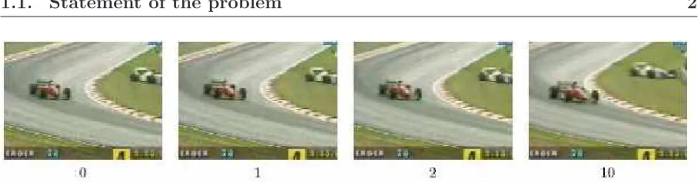
Figure 1.1: An example of successive frames in video sequences.
Visual System (HVS). In general, three types of redundancy can be identified:
Spatial redundancy or correlation between neighboring pixel values.
Spectral redundancy or correlation between different color channels or spectral bands.
Temporal redundancy or correlation between adjacent frames in a sequence of images (in video applications).
Image compression algorithms aim at reducing the number of bits required to represent an image by removing the spatial and spectral redundancies as much as possible. Image compression techniques exploit the statistical redundancies in the image and they take into consideration the human visual system imperfections [70]. Video compression, however, exploits both the temporal and spatial redundancies. Since the early 1990s, international video coding standards chronologically, H.261 [62], MPEG-1 [1], MPEG-2 H.262 [51], H.263 h263, and MPEG-4 (Part 2) [2] have been the factors behind the commercial success of digital video compression. The video documents contain an intuitive, intrinsic, and a simple idea of redundancy: two successive images with very short time intervals are very similar (see Fig.1.1). And it is indeed the research of a proper exploitation of this temporal redundancy that completely changes the scenario between still images and video sequence compression. Temporal redundancy reduction is one of the primary techniques in video compression. In the last thirty years, research efforts have concentrated on the
exploitation of the temporal redundancy using motion estimation algorithms.
The principle of the motion estimation is to find the displacement of objects between neighboring frames is estimated. The resulting motion information is exploited for an efficient inter frame coding (motion compensation). Consequently, the prediction error as well as the motion vectors are transmitted instead of the frame itself.
Block matching algorithm (BMA) is a commonly used technique in video compression to exploit temporal redundancy between successive frames. In a typical BMA, each frame is partitioned into non overlapping blocks. To exploit the video temporal redundancy, each block in the current frame is compared to all the candidate blocks in a search area of a reference frame. The candidate block that is best matched with the current block, in terms of some block-matching distortion measures, such as the sum of absolute differences (SAD) or sum square difference (SSD), is selected as the reference block for compression. The displacement between the current block and its reference block is designated by the motion vector (MV) of the current block. For compression, only the intensity and color differences between the current block and its reference block, as well as the motion vector, need to be coded. The most widely referenced block-matching algorithm is probably the full search (FS) algorithm. It finds the optimal reference block (the one with the minimum distortion measure) by evaluating exhaustively all possible candidate blocks within a search window. In so being, the FS is very computationally intensive, and thus not suitable for many real-time video applications, particularly those using software-based video compression.
More important, than video coding applications, the block matching algorithm can also be used to search the location of an object in a giving image or search area. This operation is called template matching which is the key component of object tracking, video surveillance and many related applications. The template matching task is similar to that of block matching. It finds a pattern in an image that is similar to template basis on a selected measure of similarity. The drawback of template matching is its high computational cost. In the search for an object, many small portions of an image
The present thesis remedies to the problem of the complexity of the FS in a general fashion and without using any specified application. Since we are concerned with an exhaustive matching search, we can expect that the results of the proposed methods will be similar to those already obtained by the naive full search.
1.2
Investigated approach and thesis organization
This thesis deals with the development of new rapid algorithms for block and template matching. It proposes exhaustive and fast algorithms to speed up the process of template and block matching using different metrics. Most of the proposed approaches are not based on spatial domain. They rather use the frequency domain contrary to many solutions already put forward in the literature. The proposed algorithms have a deterministic and fast execution time while still providing the same quality as an exhaustive search. They are well suited for real time applications and they benefit from the huge works that have been done in the frequency domain.
This dissertation is organized as follows.
In chapter 2, we give a survey of the state of the art of block matching algorithms. We consider the most important and efficient block matching algorithms in the literature. These latter can be divided into two main groups: The class of algorithms that reduce the number of search locations and the class which contains the fast full approaches that find the optimal solutions. Based on the insights gained from our examination and comparison of these block matching algorithms, we propose in this chapter an improved algorithm with both lossy and lossless versions using
the propriety of the temporal redundancy of motion vectors. This approach shares many concepts with the adaptive rood pattern search algorithm (ARPS). However, it gives similar or better results while reducing the computations by a factor of two.
In chapter 3, we present two simple cross correlation operations which can give ex-actly the same optimal result as the direct SSD matching algorithm. The first one makes use of the Taylor lagrange Formula to approximate the sum square difference in terms of sum of cosine difference. This latter can be computed using correlation Fourier theorem.
The second proposed approach is more simple and exact. By using some substitu-tions and complex arithmetics, The computation of SSD is derived to be a corre-lation function of two substituting functions. The former can be computed using FFT approach, which is less computationally expensive than the direct computing of SSD. The zero padding of the block is useful to avoid the circular character of FFT, and to compute the SSD function at once.
Both correlation methods are compared to many other fast spatial algorithms and existing correlation methods in terms of execution and prediction quality.
In chapter 4, a fast frequency algorithm to speed up the process of (SAD) matching is proposed. We use a new approach to approximate the SAD metric by cosine series which can be expressed in correlation terms. Experimental results demonstrate the effectiveness of this method when using only the first correlation terms for block and template matching in terms of accuracy and speed.
In Chapter 5, we describe more robust correlation techniques for local motion esti-mation purposes. They are based on the maximization of statistical robust matching functions, which can be computed in the frequency domain and, therefore, can be also implemented by fast transformation algorithms. We show that the proposed methods achieve a significant speed up and robustness over the full search block-matching algorithm under non robust metrics.
2
Block matching algorithms
2.1
Introduction
Video documents contain a large amount of temporal redundancy between the successive frames. If we can develop a good motion estimation technique and transmit only the motion information, there will be a good chance of obtaining a high compression ratio in addition to the compression achieved by processing individual frames. In the block matching algorithm (BMA), the motion estimation is carried out on a block-by-block basis. It has been adopted by such leading video compression standards MPEG 1/2/4 [1, 51, 2] and H261/263/264 [50, 65].
Generally, the optimal block matching algorithm is the full search (FS) block matching algorithm which results in the best performance with respect to the quality of decoded video sequences. However, it is computationally very intensive. Due to the huge demand of the computational requirement, several fast search algorithms have been studied over the past few decades using either sum square difference (SSD) or sum absolute difference
Three Step Search (NTSS) [56], Simple and Efficient TSS (SES) [60], Four Step Search (4SS) [68], Diamond Search (DS) [79], and Adaptive Rood Pattern Search (ARPS) [63], and so on.
The lossless algorithms contain approaches that test all candidate vectors without degrad-ing the result [57, 59, 13, 3]. These latter achieve their speedup through early elimination of candidate search positions. Most of them compute the (SAD) or SSD lower bound for the current vector, compare the best SAD or SSD found so far to the bound, and reject the candidate vector, if the lower bound is greater (worse).
The rest of this chapter is organized as follows: To have a better understanding of block matching algorithm, block matching principle is first reviewed in section 2.2. Some recent fast full search block matching algorithms are described in section 2.3,whereas some fast and lossy block matching algorithms are presented in section 2.4. In Section 2.5, an improved algorithm of the adaptive rood pattern search is proposed. In Section 2.6, simulations’ results are presented. Finally, we conclude this chapter in section 2.7.
2.2
Full search block matching algorithm
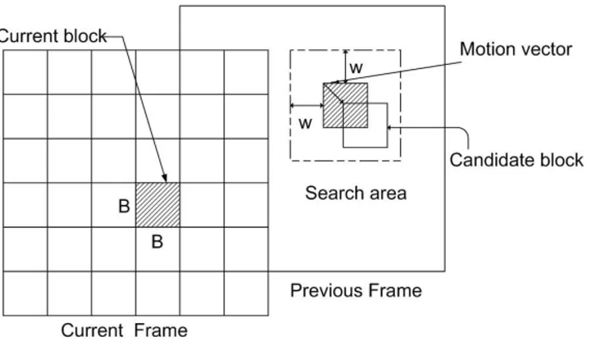
Block-matching algorithm (BMA) estimates the motion vector in a block-by-block basis. In BMA, a frame is divided into non overlapping blocks of size (B ×B) pixels. The current block in the current frame is compared with the corresponding blocks (called candidate blocks) within a search area of size (B + 2w) × (B + 2w) pixels in the previous frame, where w is the maximum displacement allowed and B2 is the block size.
The motion vectors can be estimated by using a measure of matching error. The matching error between block g and candidate blocks in a search area f is usually defined as the
Figure 2.1: Search area in block matching algorithm.
sum of absolute difference (SAD) or the sum square difference (SSD):
SAD(x, y) =B−1P l=0 B−1P k=0 |f (x + k, y + l) − g(k, l)| , (2.1) SSD(x, y) =B−1P l=0 B−1P k=0 |f (x + k, y + l) − g(k, l)|2, (2.2) where the values f (k, l) and g(k, l) denote the luminance values of f and g, and (x, y) is the candidate vector.
We briefly describe the operation of BMA between two adjacent frames in Fig. 2.1. In this chapter, only the SAD is considered as a block distortion measure. The basic operations of computing SAD are absolutions (|·|) and additions (±), and require about (3(2w + 1)2− 1) B2 operations per block where w is the maximum search window size.
Although the full search algorithm finds the motion vector which gives the global minimum of the matching error. This straightforward method takes extremely a large amount of computation. In the last years, many algorithms have been developed to accelerate the FS block matching process. We classify these techniques into two categories fast and fast full search block matching algorithms. The next section outlines the most famous fast full search block matching algorithms.
According to the triangular inequality: ||u| − |v|| ≤ |u − v| , the following inequality can be obtained: ¯ ¯ ¯ ¯ ¯ B−1X l=0 B−1 X k=0 g(k, l) −B−1P l=0 B−1P k=0 f (x + k, y + l) ¯ ¯ ¯ ¯ ¯≤ SAD(x, y) (2.3)
Let’s note G0 and F0 the sum norms of the current block and the reference block,
respec-tively, i.e.: G0 = B−1 X l=0 B−1X k=0 g(k, l) F0(x, y) = B−1P l=0 B−1P k=0 f (x + k, y + l).
So if the candidate vector (x, y) satisfies |G0− F0(x, y)| ≥ SADmin. From the
in-equality (2.3), we can deduce that this vector will not give the minimum of the SAD surface. Hence, the inequality (2.3) can be considered as providing a boundary that can omit a lot of candidates before calculating matching errors. This remark is the main idea behind the successive elimination algorithm SEA [57]. On the other hand, the sum norms can be efficiently calculated on the whole image beforehand. They can be calculated through recursive algorithms very efficiently [57].
It is obvious that at each search point, the efficiency of the SEA depends on the gap between |G0− F0(x, y)| and the SAD(x, y) in (2.3).
Partial sum norms which correspond to other smaller subblocks are present in the sum norm. Suppose G1 and F1(x, y) are partial sum norms for G0 and F0(x, y), respectively,
i.e., G0 = X i G(i)1 , F0(x, y) = X i
easily obtain the following inequality: |G0− F0(x, y)| ≤ X i ¯ ¯ ¯G(i)1 − F1(i)(x, y) ¯ ¯ ¯ (2.4)
From (2.4), several tighter boundaries can be obtained by using the partial sum norms of the subblocks. This inequality has been used to extend SEA to a multilevel case.
2.3.2
Multilevel successive elimination algorithm (MSEA)
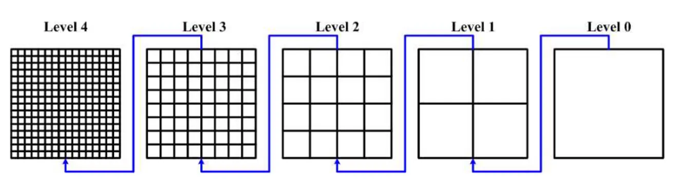
In MSEA, by dividing each block into subblocks of B
2×B2 and further into B4×B4 until 2×2,
multiple boundary levels superior than |G0− F0(x, y)| can be found. Totally, boundary
levels are obtained. All subblocks at one level have the same size. At the lth level where
0 ≤ l ≤ L, the number of subblocks is Sl= 22l = 4l and the size of each subblock is Bl×Bl
, where Bl =
B
2l. Similarly, based on triangular inequality, the following inequality can
be obtained: Sl−1X k=0 ¯ ¯ ¯G(k)l − Fl(k)(x, y) ¯ ¯ ¯ ≤ Sl+1−1X k=0 ¯ ¯ ¯G(k)l+1− Fl+1(k)(x, y) ¯ ¯ ¯ ≤ SAD(x, y) (2.5)
where G(k)l and Fl(k)denote the sum norms of the kth subblocks at the lth level in the
current block and in the reference block, respectively.
We can see from the inequality (2.5) that the boundary threshold increases
Sl−1X k=0 ¯ ¯ ¯G(k)l − Fl(k)(x, y) ¯ ¯
¯ with boundary level l and is bounded by the matching error
SAD(x, y).
In MSEA, the maximum level of such partition is Lmax = log2(B) − 1, for the blocks
with size B × B.
For B = 16, The candidate motion (x, y) is evaluated sequentially from the lowest level 0 to the highest level 3. If the candidate vector cannot be eliminated at any level between levels 0 and 3, its matching error (i.e., SAD) will be calculated at the last level. Each level allows to eliminate a certain number of candidates. The partition process in the MSEA algorithm is illustrated in Fig. 2.2.
Figure 2.2: Partition process in the MSEA algorithm.
It can be conceived that the efficient way for computation is to reject a candidate whose boundary threshold just exceeds the current SAD at the earliest possible level. Al-though MSEA can substantially reduce the computational complexity [40], two significant limitations can be seen in MSEA. Firstly, the granularity between elimination levels is coarse due to the uniform partition at each level in MSEA, and secondly the elimination process in MSEA always starts from the lowest level, although some candidates are un-likely to be rejected at lower levels. In fact, the rejection levels for neighboring candidates are reasonably correlated due to their spatial overlapping of most pixels.
To overcome these deficiencies of MSEA, a new scheme (FGSE) has been proposed [78]. The FGSE provides nondecreasing fine-grained boundary levels to reject a checking point using less computation.
2.3.3
Predictive fine granularity successive elimination (FGSE)
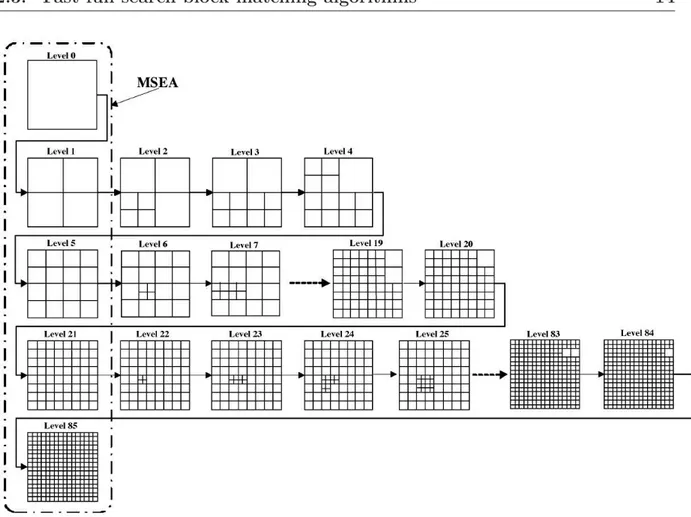
From (2.5), more partitions can yield higher boundary thresholds. In FGSE algorithm, a block of size B × B is first divided into four subblocks of equal size. Consider further partitioning each of the four subblocks one by one into four smaller subblocks of equal size. After partitioning the first subblock, they are seven subblocks (four smaller subblocks and three larger subblocks), which can give a higher boundary threshold than that given by those four larger subblocks. Larger and larger boundary thresholds can be produced as the four larger subblocks are partitioned one after another, where after each partition of a subblock, a new and larger boundary threshold is determined.
On the other hand, partitioning a single subblock into four smaller subblocks will increase the total number of subblocks by three. Subblocks of smaller size will not be partitioned further until all the other larger subblocks have been partitioned. At the same level, two different subblock sizes, m × m and (m/2) × (m/2), may exist. At the lth level
where 0 ≤ l ≤ L , the number of subblocks is Sl = 3l + 1. Then, the number of
partitioning (denoted as “Lmax ”) and the total number of subblocks (denoted as “N ”) have the relationship as 3 × Lmax + 1 = N. If we use such a partition process until the size of a partitioned subblock is 1 × 1 (pixel), we obtain N = B × B when all the partitioned subblocks are of size 1 × 1. Then Lmax = ((B × B) − 1) /3 boundary levels are established by each partition of a block/subblock of size m × m into four subblocks of size m/2 × m/2 until no more partition for size 1 × 1.
Let G(k)m×m and Fm×m(k) (x, y) denote the sum norms of the kth subblocks of size m × m
in the current block and in the reference block, respectively. The kth subblock is divided
into four subblocks of equal size, the sum norms of which are denoted as G(4k+2j+i)(m/2)×(m/2)and
F(m/2)×(m/2)(4k+2j+i) (x, y), respectively, i, j = 0, 1. Then, the following inequality holds: ¯ ¯ ¯Fm×m(k) (x, y) − G(k)m×m ¯ ¯ ¯ ≤ 1 X j=0 1 X i=0 ¯ ¯ ¯F(m/2)×(m/2)(4k+2j+i) (x, y) − G(4k+2j+i)(m/2)×(m/2) ¯ ¯ ¯ . (2.6)
The boundary threshold at level l as BTl is given by:
BTl(x, y) = S1−1X k=0 ¯ ¯ ¯Fn(k,l)×n(k,l)(k) (x, y) − G(k)n(k,l)×n(k,l) ¯ ¯ ¯ . (2.7) where n(k, l) × n(k, l) is the size of the kth subblock at level l. As mentioned above,
n(k, l) × n(k, l) may be m × m or (m/2) × (m/2), depending on subblock index k and level l. As l increases by 1, there is one more subblock of size m × m being partitioned into
four smaller subblocks of size (m/2) × (m/2). Therefore, based on the inequality (2.6), the following relationships can be obtained:
Figure 2.3: Partition process in the FGSE algorithm where there are 86 levels in total
in contrast with only five levels (level 0, level 1, level 5, level 21, and level 85) in MSEA.
Equation (2.8) means that boundary threshold BTl increases with the level l, and all
boundary thresholds are inferior to the matching error SAD(x, y). But, the calculation of BTl requires more computations as l increases.
For block size of 16 × 16, Lmax = 85. This implies that 85 boundaries excluding that at level 0 without partition. SAD (matching error) is calculated at level 85. The partition process in the FGSE algorithm is illustrated in Fig. 2.3.
Since two adjacent checking points (blocks) have most of the block pixels with just one pixel shifting horizontally or vertically, the authors in [78] have also developed a scheme to predict the rejection level for a given candidate by exploiting the correlation of matching errors between two adjacent motion vectors. Then, the resulting predictive FGSE algorithm can further reduce the computation load by omitting some redundant
Figure 2.4: The group of pixel locations for the calculation of the partial distortion
dp(x, y). sp, tp are the offsets of the upper left corner point of the partial block.
boundary levels.
2.3.4
Normalized PDS (NPDS) algorithm
So as to reduce the number of computations, the previous cited algorithms can be coupled with halfway-stop techniques. One of the examples is the partial distance search algorithm (PDS) [8]. The basic idea behind this algorithm is that the input vector consists of many partial distortions. The total distortion is obtained by adding these partial distortions. If the pth accumulated partial distortion is greater than the current minimum distortion,
this vector is rejected, and the remaining partial distortions are not calculated. However, the efficiency of this algorithm is limited in motion estimation.
Recently, normalized partial distortion search (NPDS) [15] has been proposed. This algorithm reduces computation by using a halfway-stop technique in the BDM calculation similar to the PDS algorithm. The major difference from the PDS algorithm is that NPDS normalizes the accumulated partial distortion and the current minimum distortion before
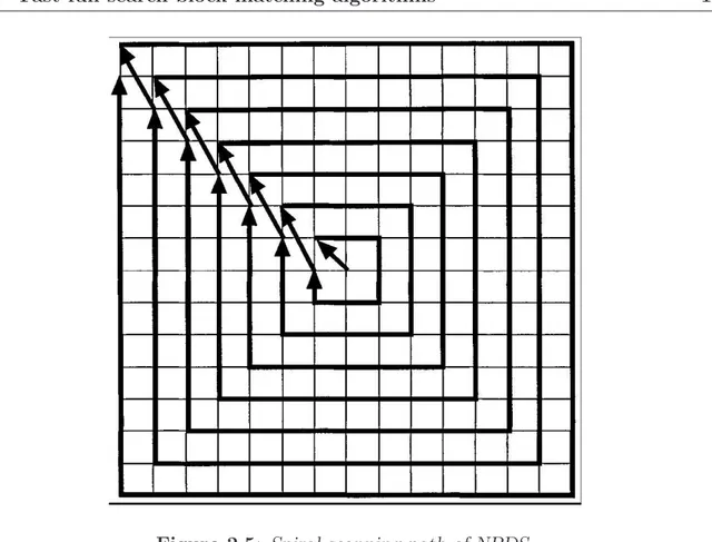
Figure 2.5: Spiral scanning path of NPDS.
comparison. The probability of early rejection of nonbest candidate motion vectors is thus increased.
Supposing that the block size is equal to 16 × 16, in NPDS, the block distortion SAD is divided into 16 partial distortions (dp) [14], where each partial distortion consists of 16
points spaced equally between adjacent points, as shown in Fig. 2.4.
D(x, y) = P15 l=0 15 P k=0 |f (x + k, y + l) − g(k, l)| , (2.9)
The pth partial distortion is defined as
dp(x, y) = 3 P l=0 3 P k=0 |f (x + 4k + sp, y + 4l + tp) − g(4k + sp, 4l + tp)| , (2.10)
where (sp, tp) is the offset of the upper left corner point of the pth partial distortion from
the upper left corner point of the block( Fig. 2.4). The pthaccumulated partial distortion
is defined as Dp(x, y) = p X i=1 di(x, y). (2.11)
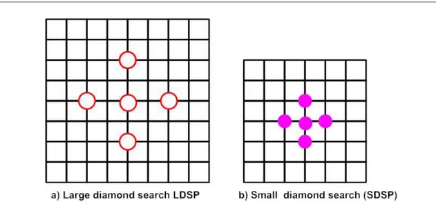
Figure 2.6: LDSP and SDSP patterns.
The NPDS matches all the checking points inside the search window as the FS algo-rithm. The search begins at the origin checking points and moves outwards with a spiral scanning path (see Fig. 2.5). During each block matching, the NPDS compares each accumulated partial distortion Dp with the normalized minimum distortion (pDmin/16).
Comparison starts from p = 1 to p = 16, and is stopped if the normalized partial dis-tortion of the current motion vector is greater than the normalized minimum disdis-tortion. This is called the halfway stop in NPDS [15]. At the end of the comparison (i.e., p = 16), if D16 is smaller than pDmin/16, then this current motion vector becomes the new
cur-rent minimum point. By comparing the normalized partial distortion to the normalized minimum distortion, computational complexity is reduced by the elimination of nonbest motion vectors at an early stage. The NPDS, however, limits the maximum possible speedup to 16 times theoretically.
2.4
Fast Block matching algorithms
2.4.1
Diamond Search (DS)
The DS algorithm uses two search patterns as illustrated in Fig. 2.6, which are derived from the crosses (×). The first pattern, called large diamond search pattern (LDSP), con-tains nine checking points from which eight points surround the centeral one to constitute
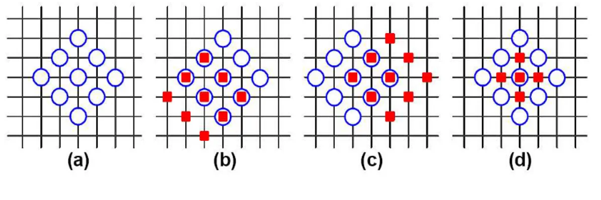
Figure 2.7: Diamond Search.
a diamond shape. The second pattern consisting of five checking points forms a smaller diamond shape, called small diamond search pattern (SDSP).
The DS begins from the original center of the search window by evaluating the SAD measure at nine checking points as shown in Fig. 2.7(a). If the minimum SAD is not found at the diamond center, depending on its location, three or five additional points are checked for the next minimum SAD [see Fig. 2.7(b) and Fig. 2.7(c)]. The operation is repeated until the minimum SAD is found at the diamond center. Then, another four checking points around the current minimum SAD are evaluated to determine the final reference block and hence the motion vector (see Fig. 2.7(d)). The DS usually gives better results than the existing TSS and NTSS algorithms. It reduces considerably the number of checking points while keeping or without degrading much the video quality, especially for video sequences with small motion [80].
However, the DS is not suitable for sequences with large or complex motion. Indeed, the DS does not exploit the motion correlation between adjacent frames or blocks. It also evaluates exhaustively all eight neighboring points around the diamond center; and it cannot stop the search early even when the SAD at a particular checking point is already small.
A number of algorithms have been proposed to improve the performance of DS algo-rithm by addressing one, two, or all the three limitations mentioned above. Some of them have achieved very important results in terms of reducing the computational complexity like the hexagonal search (HEXBS) [77] or reducing the computational complexity and
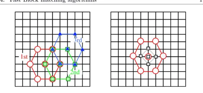
Figure 2.8: Hexagonal search.
improving the video quality like the adaptive rood pattern search (ARPS) and adaptive irregular pattern search (AIPS) [63, 64]. In the following subsections, we review three of these state-of-the-art algorithms.
2.4.2
Hexagonal Search (HEXBS)
In order to reduce the number of points to be checked in each search step, the HEXBS uses an hexagonal pattern instead of large diamond search pattern. It starts by evaluating seven checking points of a hexagon centered at the original center of search window as shown in Fig. 2.8(Left). If the minimum SAD is not achieved at the hexagon’s center, the search is repeated by centering the hexagon at the point of minimum SAD and evaluating the three new endpoints of the hexagon. When the minimum SAD occurs at the hexagon’s center, four adjacent points around the center are checked to determine the final best-matched point as illustrated in Fig. 2.8(right). Simulation results reported in [77] show that the HEXBS could achieve a notable speed-up gain compared with the DS at the expense of little degradation in video quality in terms of peak signal-to noise ratio (PSNR).
2.4.3
Adaptive Rood Pattern Search (ARPS)
The ARPS algorithm evaluates the four endpoints of a four-armed rood pattern, together with the point indicated by the motion vector (MV) predicted from those of the adjacent
Figure 2.9: Initial region search in ARPS algorithm.
blocks (only the left block is suggested in [63]), all centered around the original center of the search window (see Fig.2.9). A unit-sized rood pattern is then centered at the point of minimum SAD found in the initial step, and its four endpoints are evaluated and compared with the SAD at the center point for the new minimum SAD. This step is applied until the minimum SAD is found at the center. In addition, an early termination scheme called zero-motion prejudgment (ZMP) is included in the initial step. Below is a pseudo code of the ARPS-ZMP algorithm.
Let L be the size (the length of each arm) of the rood pattern.
Step 1: Compute the SAD at the original center (0, 0) of the search window. If SAD(0, 0) is less than a threshold T (T = 512)
MV = (0, 0);
Stop; Else
If the current block is a leftmost block of the frame, Set L = 2 ;
Else (the current block is not a leftmost block) Set L = max(|mvx|, |mvy|)
where |mvx|, and |mvy| are, respectively, the x and y components of the predicted
Figure 2.10: Adaptive irregular pattern search.
Step 2: Evaluate the four endpoints at (+L, 0), (−L , 0), (0, +L ) and (0, −L ), plus the point indicated by the predicted MV (x) to locate the point of minimum SAD (see Fig.2.9).
Step 3: Evaluate the four endpoints of a unit-size rood pattern centered at the point of minimum SAD found in Step 2. If the new minimum SAD is not found at the center, repeat this step; otherwise, select the MV corresponding to the current center as the final solution. The ZMP scheme reduces the number of checking points by terminating early the search for stationary blocks, i.e., blocks with zero motion vector.
2.4.4
Adaptive irregular pattern search (AIPS)
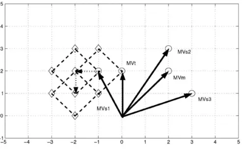
In [64], a simple fast block matching algorithm (BMA), called adaptive irregular pat-tern search with matching prejudgment (AIPS-MP), is proposed. In the AIPS-MP, a dynamic search pattern, called adaptive irregular pattern (AIP), is constructed for each block based on its spatial and temporal neighboring motion vectors (MVs), namely three MVs provided by the spatial neighboring blocks (denoted by MVs1, MVs2, and MVs3, respectively, in Fig. 2.10, for example), their median MV (denoted by MVm) and the temporal neighboring MV (denoted by MVt). The AIP is used to quickly identify the
adopted in the MPEG-4 Verification Model and the Optimization Model, respectively, on the average PSNR and the search speed.
2.5
Proposed algorithm (DMPS)
2.5.1
Overview
Based on the insights gained from our examination and comparison of the ARPS al-gorithm, we propose in this chapter an improved algorithm in both lossy and lossless versions, which we call Dominant Pattern Search Algorithm (DMPS). As the name sug-gests, DMPS uses the most dominant vectors already found in the previous frame. As we can see later, this algorithm can reduce markedly the computational complexity while still keeping the same video quality as the ARPS algorithm.
Our proposed algorithm makes use of three following points to achieve high perfor-mance.
1) Initial Region Search (IRS): In temporal prediction, it is assumed that local object region or video scene moves with similar motion over consecutive frames. Conse-quently, the motion vector of the same block and the most frequent vectors components in the previous frame can be used to predict the MV or IRS for the current block. The one with the least SAD is identified as the initial region search (IRS) to find the optimal motion vector.
2) Early search termination: After the IRS has been identified, it should be decided whether it is likely to be ‘good enough’ as the optimal solution by comparing its SAD with a pre-determined threshold, so that the search could be terminated at this
Figure 2.11: Example of search pattern of DMPS.
early stage to reduce the computational cost.
3) Refined search: As the proposed IRS prediction scheme is rather accurate, we found that it is efficient to evaluate the endpoints of a small (2 × 2) cross pattern and repeat the search until the minimum is located at the center of the small cross diamond.
2.5.2
Initial region search
To construct the IRS, we resort to the temporal block and to the most frequent horizontal and vertical components, because they are often associated with the same object and have similar MVs as that the current block. Choosing appropriate vectors to form the initial region search (IRS) is the key element of the DMPS that improves its performance over the ARPS. In the ARPS [63], the IRS constitutes only the immediate-left neighboring block in the current frame. However, the left neighboring block is not always correlated with the current block and unavailable for the left-margin blocks. Moreover, only the magnitude of the neighboring MV is used to control the arm size of the ARP, while the MVs direction is not utilized. By considering these two aspects, the PSNR performance of the ARPS can be further improved, especially for those large motion sequences. Therefore, larger IRS and more proper utilization of their MVs (i.e., both magnitude and direction) would be
frequent temporal horizontal and vertical motion vectors components are also made use of.
Let mvp
x(i, j) and mvyp(i, j) be the motion vectors already found in the previous frame
and let Histp
x and Histpy be the histograms presenting the frequencies of horizontal and
vertical components of the motion vectors respectively. These histograms can be obtained progressively during the motion estimation process of the previous frame. They require just two operations of additions per block. Let’s F m1
x, F m1y be respectively the most
frequent horizontal and vertical components vectors in the reference frame followed by
F m2
x, F m2y. In this algorithm, the IRS is constructed by using the temporal vector of the
same block in the reference mvp
x, mvyp and four vectors calculated from F m1x, F m1y and
F m2
x, F m2y. An example of the initial region search in DMPS algorithm is presented in
Fig. 2.11.
2.5.3
Early search judgement
To further speed up the search, some BMAs terminate the search once the matching error is lower than a predetermined threshold. For example, the ARPS [63] first checks the search point located at the center of the search window and stops the search immediately once the matching error yielded reaches below the chosen threshold 512. This checking process is called zero-motion prejudgment (ZMP), with a fixed threshold. Note that the MVFAST [48] also performs such a checking.
In the DMPS method, we use an adaptive threshold using the block distortion of the reference frame. The threshold is chosen as the minimum value of the distortion measure in the area including the 8 blocks in the reference frame. If the threshold computed is
Figure 2.12: Refined search pattern.
inferior to 512, then 512 is adopted as the current threshold for the current block.
The proposed approach for early search termination can further reduce the compu-tational cost for most types of blocks, not just stationary blocks (i.e. block with zero motion vector) as in the ARPS algorithm. This is because the distortion measure of the blocks in the current frame is highly correlated with that of the neighboring blocks in the reference frame.
2.5.4
Refined search
2.5.4.1 Lossy search
In the literature, most BMAs that explore the inter-block correlation perform their refined search using a fast BMA based on a set of fixed search patterns. A representative example is the motion vector field adaptive search technique (MVFAST) [48, 54, 68]. In our view, since the refined search center identified by the DMPS is already close to the global MME point, any local search using a small compact search pattern should be fairly efficient. We exploit the five-point small diamond search pattern (SDSP) [80] for the refined search, which is also used in the ARPS and shows excellent performance.
In Fig. 2.12, a sample refined search path of the DMPS is demonstrated. The point with the minimum SAD of each SDSP is used as the center of the SDSP in the next refined search iteration. There are totally three SDSPs illustrated in this example. Furthermore,
In order to obtain a lossless search, after choosing the motion vector with minimum SAD in the IRS, we refine the search by using the successive elimination method SEA. A look-up map is employed to record whether a search points has been checked in order to avoid duplicated search. Using this version of the algorithm, we expect to find the same result as an exhaustive algorithm.
2.6
Simulations
In our simulations, the BDM is defined to be the mean peak signal to noise ratio (PSNR). The block size is 16 × 16, and the maximum displacement in the search areas is ±7 pixels in both the horizontal and the vertical directions. The simulation is performed with a total of six sequences with different degrees and types of motion content. We compared the DMPS using threshold (T = 512) and DMPS using adaptive threshold (DMPS1) against FS, SEA, TSS, FSS, NTSS, DS, and ARPS using the following test criteria:
1) Average searching point (SP) – the average number of search points used to find the motion vector; and 2) Average peak signal to noise ratio (PSNR)– This shows the quality of prediction.
Table 2.2 and 2.1 summarize the experimental results of each search strategy over the test criteria using the 6 tested sequences.
By observing the result obtained in Table 2.1, the DMPS takes the smallest average number of search points per block (i.e. the fastest algorithm) among other fast BMA for the entire six test sequences.
Table 2.1: Simulations results of BMAs in terms of number of SPs per block
Sequence FS SEA DS TSS FSS NTSS ARPS DMPS DMPS1
Carphone 184.56 88.23 12.97 21.60 15.62 16.75 6.78 4.33 4.26 Foreman 184.56 91.05 13.20 21.63 15.88 16.88 6.80 4.75 4.69 Stefan 184.56 134.04 14.83 21.67 16.72 19.36 7.96 5.25 5.07 M&D 184.56 86.61 11.92 21.51 14.99 15.39 5.52 2.13 2.13 Table 184.56 119.28 12.87 21.63 15.70 16.52 6.52 4.06 4.02 News 184.56 84.05 11.62 21.48 14.77 14.94 5.15 1.80 1.79
Table 2.2: Simulations results of BMAs in terms of ∆PSNR (dB) (FS shows actual
PSNR)
Sequence FS SEA DS TSS FSS NTSS ARPS DMPS DMPS1
Carphone 33.71 0.00 -0.10 -0.18 -0.18 -0.07 -0.18 -0.19 -0.20 Foreman 32.41 0.00 -0.19 -0.30 -0.23 -0.11 -0.30 -0.26 -0.26 Stefan 25.24 0.00 -0.49 -0.23 -0.46 -0.18 -0.20 -0.08 -0.08 M&D 39.63 0.00 -0.05 -0.08 -0.04 -0.03 -0.07 -0.07 -0.07 Table 29.87 0.00 -0.29 -0.29 -0.34 -0.23 -0.52 -0.53 -0.54 News 36.52 0.00 -0.04 -0.04 -0.05 -0.03 -0.08 -0.08 -0.09
ARPS and sometimes even better while significantly reducing the computational cost for most types of blocks, not only stationary blocks (i.e. block with zero motion vector) as in the ARPS algorithm. This is because both zero and non-zero motion vectors that are highly correlated with the most frequent temporal motion vectors can be well predicted by the proposed IRS prediction scheme.
2.7
Conclusion
In this chapter we have outlined the most recently efficient block matching algorithms. We have also proposed an improved algorithm for fast block matching. Our method (DMPS) is based on the temporal correlation between the motion vectors and the cross
3
Exhaustive SSD matching using frequency
domain
3.1
Introduction
Sum square difference (SSD) metric has been applied to many areas of image and video processing such as image registration, motion compensated video compression, multi-frame image enhancement, remote sensing, and many computer vision tasks. The prob-lem of SSD translational image matching is a specific case of the more general probprob-lem of estimating motion in an image sequence.
In this chapter, we focus on translational image motion using sum square difference met-ric(SSD). Even though this motion model is very simple, it is a key element of various video processing tasks. More importantly, it is a critical component of many video pro-cessing and compression systems.
In this chapter, we are interested in solving the problem of full search block matching
which has become one of the motion estimation methods of choice for a wide range of professional studio and broadcasting applications. A variant of correlation methods have been proposed over the years. Even these type of algorithms can present many attractive applications for motion estimation. But when the goal is the minimization of the SSD metric as the case for the most spatial block matching algorithms, these methods are unable to give the same solution as the direct search. Also even the correlation operations can be used to evaluate the SSD criterion [12,27,53]. However, to our knowledge no one has solved the problem of non cyclic SSD matching using only one correlation operation. The aim of this chapter is to show the existence of new and very simple correlation methods for SSD computation. though the correlation operation is quite expensive in computing directly (O(N2) for two 1D signals of length N), it can be performed much more efficiently
via the frequency domain (O(NlogN )) by taking advantage of the Fast Fourier Transform (FFT). Computing Fourier transforms quickly has been the task of much work over the last 50 years. Off-the-shelf code [37], DSP chips with custom algorithms, and even full custom micro-chips based on [17] are readily available.
In order to make the present chapter self contained, section 3.2 reviews existing cor-relation and Fourier related methods. Section 3.3, presents our proposed corcor-relation techniques. Section 3.4 presents performance results. Finally some concluding remarks are drawn in section 3.5.
3.2
Fourier and correlation based methods
3.2.1
Translational motion in the Fourier domain
It has well known that a pure displacement corresponds to a phase shift in the frequency domain. Let us consider two successive frames which differ only by shift (x, y):
f (k, l, t) = f (k − x, l − y, t − 1) (3.1)
Taking the discrete Fourier transform (DFT) on (k, l), we get:
Ft(u, v) = Ft−1(u, v) exp(−jux − jvy) (3.2)
Where Ft( .) ) and Ft−1( .) are the 2-D Fourier transformations of the current frame and
previous frame, respectively. On the other hand we have:
Ft(u, v) = |Ft(u, v)| exp(j. arg[Ft(u, v)]) (3.3)
Ft−1(u, v) = |Ft−1(u, v)| exp(j. arg[Ft−1(u, v)]) (3.4)
The shift (x, y) is contained in the phase difference. To compute it, we take the phase difference between the previous frame’s transform and the current frame’s transform. From ( 3.2), we obtain:
∆φ(u, v) = arg[Ft(u, v)] − arg[Ft−1(u, v)] = −ux − v y (3.5)
Theoretically, the evaluation of this equation at only two independent frequency points allows us to obtain the displacement (x, y). In practice, the estimation of the displace-ment should be computed using several points to reduce noise effect (including object deformation). In calculating the phase difference, there is an ambiguity of integer multi-ples of 2π. This ambiguity is one of the problems to be tackled in using (3.5). However, This frequency component formulation has not attracted much attention over the past 20 years. The most well-known Fourier based method is the so called phase correlation.
(a) Current frame (b) Cross correlation (CORR) (c) Phase correlation (PC)
(d) Fast robust correlation (FR-corr)
(e) Orientation correlation (OC) (f) Full search using SSD metric (FS)
Figure 3.1: Reconstructed frame from Carphone cif sequence using different correlation
methods for block size 162 and corresponding search range of ±8.
3.2.2
Correlation based methods
3.2.2.1 Phase correlation
Cross correlation has been known from many years as one of the most common ways for template and image matching. The baseline cross correlation operates on a pair of images ft and ft+1 of consecutive frames or fields of moving sequence sampled at t, t + 1.
The estimation of motion relies on the detection of the maximum of the cross correlation function between ftand ft+1. Since all the functions involved are discrete, cross correlation
implementations. The correlation surface is defined as:
< {IF F T (F (ft)F∗(ft+1))} . (3.6)
A more accurate correlation technique is the phase correlation [55]. This method has been firstly proposed to estimate translation between two displaced images and was found to be able to measure large motions. It is based on the shift property of Fourier transform which states that translation in spatial domain corresponds to phase shift in frequency domain. In the phase correlation method, the translational motion vector is measured from the position of the maximum of the following surface:
< ½ IF F T µ F (ft)F∗(ft+1) |F (ft)F∗(ft+1)| ¶¾ . (3.7)
The most remarkable property of the phase correlation method compared to the classi-cal cross correlation method is the accuracy by which the peak of the correlation function can be detected. In addition, phase correlation offers key advantages in terms of its strong response to edges and salient picture features, its immunity to illumination changes and moving shadows and its ability to measure large displacements.
3.2.2.2 Gradient correlation techniques
In this section, we recall the principle of the gradient based correlation techniques. The use of the images gradient for motion estimation goes back to an old date. It had at the beginning like application the image registration. In this section we insist on two methods recently published which are gradient correlation and orientation correlation.
Gradient correlation This method estimates the movement between two successive frames ftand ft+1from the calculation of the gradient correlation in the frequency domain
[5, 6].
The gradient of the image ft is a complex image gt which is defined as follows:
gt(x, y) =
∂f (x, y)
∂x + i
∂f (x, y)
The position (k, l) which maximizes (3.9) denotes the translation between the compared frames. In the same manner as the block matching algorithms the gradient correlation can be applied as a block based approach for local motion estimation.
Orientation correlation The orientation correlation (OC) has been recently proposed in [33]. This method estimates the motion between ft and ft+1 from the gradient
orien-tation .
The gradient orientation of the frame ft is a complex image fd,t defined as follows:
fd,t(x, y) = sgn( ∂ft(x, y) ∂x + i ∂ft(x, y) ∂y ) (3.10) wheresgn(x) = 0 if |x| = 0 x |x| elsewhere
The gradient orientation fd,t+1 of ft+1 is defined in the similar fashion as fd,t.
The method (OC) computes the correlation between fd,t and fd,t+1 in the frequency
domain.
Let FD,t(u, v) be the FFT of fd,t+1(x, y), FD,t+1(u, v)the FFT of fd,t+1(x, y) and IF F T ()
be the inverse Fourier transform, the correlation of the orientation is defined as follows:
<©IF F T (F∗
d,t(u, v)Fd,t+1(u, v)
ª
. (3.11)
The position (k, l) which maximizes (3.11) indicates the translation motion between the compared images. As it has been reported in [33], the orientation correlation method exceeds the phase correlation for both local and global motion estimation, however the efficiency of this correlation is still sub optimal when compared with the full search block matching algorithm.
3.2.2.3 Fast robust correlation
A new recent robust cross correlation ”Fast robust correlation” has been recently proposed in [34]. The fast robust correlation applies a kernel based on the M-estimator proposed by Andrews [49] to differences intensities. Fast robust correlation works by expressing a robust matching surface as a series of correlations. Speed is obtained by computing correlations in the frequency domain. Three experiments showing the advantages of fast robust correlation over the standard correlation have been presented. These have been found in block motion estimation for video coding, video frame registration and tolerance of rotation and zoom. Orientation correlation” already cited above works by correlating orientation images using the Andrew’s wave M estimator. In this method, angles of gradient orientation are matched using Andrew’s robust kernel [33].
The existing correlation methods can present many attractive features such as fast execution time due to the use of FFT algorithms as well as insensitivity to illumination for the phase correlation and robustness to outliers for ”Fast robust correlations”. However, when the goal is to search the optimal vector which minimizes the SSD metric, the previous correlation methods fail to guarantee the same level of performance as the spatial direct full search algorithm (see Fig. 3.1). These methods can only work as a first approximation and must be followed by a spatial search to refine the motion vector found ”image correlation” [58]. In the section 3.3, we show two simple cross correlation methods with optimal accuracy as the FS algorithm.
3.2.3
Frequency components
The phase correlation takes all the frequency components into consideration at the same time. To illustrate the intrinsic properties of motion estimation we refer to (3.5) and analyze the contribution of individual components in the motion estimation process. It is obvious from (3.5) that:
(uv) Ã x y ! = −∆φ(u, v). (3.12)
Now, we want to know the noise effect. Considering that the total noise of various sources can be modeled as a noise n(.) , added to (3.1),
f (k, l, t) = f (k − x, l − y, t − 1) + n(k, l). (3.14)
By using Fourier series n(.) can be represented as
n(k, l) =X X|N(m1, m2)| e j 2π Wm1k+ 2π Hm2l+φn(m1,m2) , (3.15)
where φn(m1, m2) is the phase of N(m1, m2). By representing f (., ., t) and f (., ., t − 1)
by their Fourier series, (3.14) becomes
|Ft(m1, m2)| e j(2π Wm1k+ 2π Hm2l+φt(m1,m2)) = |Ft−1(m1, m2)| e j(2π W m1k+ 2π Hm2l+φt−1(m1,m2)) + |N(m1, m2)| e j(2π Wm1k+ 2π Hm2l+φn(m1,m2))
From this latter, we obtain
|Ft| = £¡ |Ft−1| + |N| cos(φn− φt−1) ¢2 +¡|N| sin(φn− φt−1)¢2¤1/2 (3.16) φt = φt−1− (2π Wm1x + 2π Hm2y) + arctan µ |N| sin(φn− φt−1) |Ft−1| + |N| cos(φn− φt−1) ¶ (3.17)
These equations are identical to the noise analysis in the phase modulation or the fre-quency modulation systems in communication. For |Ft−1| >> |N|, the noise disturbance
to the phase information is less than its effect on the original signal. This is the well known noise-reduction property of continuous phase modulation. Therefore the displace-ment estimate based on phase information is less sensitive to noise than that based on
the original signal, provided that the signal magnitude is much higher than the noise one. However, this noise-reduction situation is reversed when the noise magnitude is close to or higher than the signal magnitude. In this case, the phase information suffers more distortion than the original signal. This is the well known “threshold effect’ in continuous phase modulation. The preceding analysis, therefore, tells us that we should avoid using the phase information at those frequencies for which the signal power is not much higher than the noise power. On the other hand, our desired information, (x, y), is scaled by (m1, m2) in the phase component. For example, if m1 = 0 and |Ft−1| >> |N| in (3.17),
then y = − H 2π∆φ m2 + H 2πarctan µ |N| sin(φn) |Ft−1| ¶ m2 (3.18) The higher frequency components are more efficient in vector motion estimation because the second (noise) term is divided by m2. However the high frequency component has
short (spatial) cycles which corresponds to the ambiguity problem. The exact shift may be equal to the estimated phase value plus an integer number of cycles.
3.3
The proposed algorithms
3.3.1
Mathematical background:
In a block matching algorithm, the current frame is partitioned into square blocks B ×
B. Assuming that each block undergoes translational motion, a block motion vector is
estimated for each block to describe its two-dimensional (2-D) translation. For a given block g in the current frame a search is made in the reference frame over a search area
f within a fixed-sized of search window ±w. The objective is to search for the best
matching block which gives the least prediction error and which usually minimizing either sum absolute difference (SAD), or sum square difference (SSD). In this chapter, we are concerned with the SSD criterion.