Accounting for coherence in wind forces in finite element models

(1)

Accounting for coherence in wind forces in finite element models

V. Denoël

Département de Mécanique des matériaux et Structures, Université de Liège, Belgique

ABSTRACT: The behaviour of civil engineering structures subjected to wind forces is generally approached by means of finite element models. These numerical models are necessary since the shape of the structure as well as the representation of the applied forces are difficult to handle in closed forms.

In stochastic dynamic analyses, the coherence of the applied forces – in this context coming from the wind flow – is represented by the off-diagonal terms in the power spectral density matrix. This matrix is obtained by assembling elementary matrices, each of them corresponding to a stochastically loaded finite element. Even though the unique rigorous approach is not so complicated, simplified formulations are generally used to set up these elementary matrices. These simplifications result in a bad estimation of the high frequency content of the applied forces. Comparing these approached power spectral density’s to the actual ones en-ables to determine numerical admittance functions which allow correcting the bad estimation of the forces. This paper presents several finite element formulations for the estimation of the applied forces and derives the corresponding expressions of the numerical admittance functions.

1 INTRODUCTION

Dynamic forces acting on structures are not always perfectly determined. This is for instance the case when the loading comes from natural phenomena (earthquake, wind, waves…) or from human activi-ties (walk, traffic …). The force acting at a point of the structure must therefore be described in a prob-abilistic way. Moreover, it is necessary to character-ize the coherence that may exist between forces act-ing at different points.

The analysis of the structure, which consists es-sentially in computing its displacements, must take this coherence into account. For very simple struc-tures and simple coherence fields, this can be achieved in an analytical way. For more complex structures, the analysis must necessarily be realized with a numerical procedure.

The goal of this paper is to discuss the precision that can be achieved with finite element models in the representation of the coherence field.

The first paragraph is dedicated to the presenta-tion of the wind loading. This domain of applicapresenta-tion has been chosen but the developments presented in this paper could also be applied to other domains where the coherence of pressures has to be ac-counted for.

In a second step, we will present analytical devel-opments on a very simple structure and an example of a particular finite element formulation. Finally, we will compare results obtained with these two methods and discuss the limit of applicability of the finite element method.

2 STATISTICAL CHARACTERIZATION OF WIND PRESSURES

The power spectral density (PSD) of the wind pres-sure acting in a section of a structure can be ex-pressed in terms of the PSD of the wind velocity in the same section:

( )

n s S

( )

n s

S_p , =γ2 _u , (1)

where γ =0.5ρC_DBU represents the aerodynamic properties of the cross section, n represents the fre-quency (in Hz) and s stands for the section abscissa.

The coherence of wind pressures applied at two different sections of the structure can be expressed by the cross-correlation:

(

n,s1,s2

)

S

(

n,s1

) (

S n,s2

) (

n,s1,s2

)

S_p = _p _p Γ (2)

where Γ

(

n,s1,s2

)

represents the coherence function between pressures (and hence wind speeds) at sec-tions s1 and s2.

(2)

In wind applications, it is generally assumed that the coherence function is exponentially shaped (Dyrbye and Hansen 1997):

(

)

U s s Cn e s s n 2 2 1 2 1 , , − − = Γ (3)

where C and U are respectively the coherence co-efficient and the mean wind speed. Note that this shape is physically acceptable since the coherence function is equal to unity (Γ=1) for quasi-static components (n=0) or for identical sections (s₁ =s₂) and is monotonically decreasing with the distance between two points and with the frequency. 3 ANALYTICAL DEVELOPMENTS

We will limit our developments to a wind field with uniform probabilistic characteristics: let us suppose that the mean wind velocity and the PSD of the wind velocity are the same at every point of the structure.

The structure that will be studied is a beam lying on simple supports and its transverse displacements only will be computed. Let us also suppose that the cross section is symmetric in such a way that the drag forces only have to be taken into account.

If the pressures applied on the structure p

( )

t were deterministic, i.e. if the evolution in time of the pressures was known, their projection into the modal basis could be obtained by:

( )

=

_∫

L i ds L s i s t p t p 0 * sin ) , ( π (4)

where i is the mode in which the projection is real-ized. In a stochastic analysis context, this projection must be realized in terms of power spectral densities. The elements of the PSD matrix (PSDM) of the gen-eralized forces can be expressed by:

( )

=

_∫∫

L L _p

(

)

F _L dsds s j L s i s s n S n S ij 0 2 0 1 2 1 2 1, sin sin , * π π (5) With the limitations of the wind field considered in this paper, this relation is:

( )

n S

( )

n L

( )

n S_F _u _ij ij = Ψ 2 2 * γ (6) where

( )

=

_{∫ ∫}

− − Ψ L L U s s Cn ij dsds L s j L s i e L n 0 2 0 1 2 1 2 2 sin sin 1 1 2 π π (7) is a non dimensional function representing the re-duction of the applied pressures when they are pro-jected to modes i and j . These functions are called “mechanical admittances” (Fig. 1).

This figure shows for example that the projection of the pressures applied on the beam in the first

mode (i=j=1) will result in a reduction of the higher frequency content. 0 2 4 6 8 10 0 0.05 0.1 0.15 0.2 0.25 0.3 0.35 0.4 0.45 C n L / 2 U i = j = 1 i = j = 2 i = j = 3 i = j = 4

Fig. 1: Examples of mechanical admittances

When the PSDM of the generalized forces is known (Eq. 6), the PSDM of the generalized coordinates can then be expressed (Clough, Penzien 1993) as a function of the transfer functions in each mode. We will however limit the presentation here since, in the following, we will compare the PSD’s of the gener-alized forces only.

4 FINITE ELEMENT MODEL

Equation (1) shows that the force applied at a node of the finite element model can be expressed by:

( )

t s u

( )

t s

p , =γ , (9)

It is usual, in a finite element context, to consider the global displacements and deformations of a whole structure in terms of what happens at the nodes. It is thus tempting to consider wind velocities u(t) at the nodes of the model only. The knowledge of the wind velocity at these points allows determining the wind pressures at the nodes of the structure. In a stochas-tic analysis, the PSDM of these forces can be ex-pressed in a very simple way.

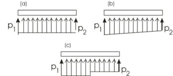
p₁ _p 2 p₁ _p 2 p₁ _p 2 (a) (b) (c)

Fig. 2: Examples of hypotheses on the pressure distribution along a finite element - (a) Constant mean pressure (b) Linear variation (c) Bi-rectangular variation.

Since the wind pressures are known at the nodes of the finite element only, hypotheses must be for-mulated concerning the pressure distribution along the element. Fig. 2 represents some examples.

Further developments are based on a bi-rectangular variation of the pressure (Fig. 2-c). The nodal forces are thus expressed by:

(3)

(

1 2

)

2

(

1 2

)

1 3 13 32 ; 3 13 32 p p l F p p l F = + = + (10)

where l stands for the length of the finite element, p1

and p2 represent wind pressures at the nodes and F1

and F2 are the nodal forces. After rotation and

local-ization (usual procedures in finite elements devel-opments, Zienkiewicz 2000), these relations allows to express the nodal forces in terms of the wind ve-locities. The PSDM of the nodal forces can thus be expressed in terms of the PSDM of the wind veloci-ties at the nodes of the structure:

{ }

[ ]

{ }

[ ] [ ][ ][ ]

T u F M S M S u M F = ⇒ = (11)

As in the analytical procedure, the PSDM of the generalized forces can then be obtained:

[ ]

=

[ ] [ ][ ]

ΦT _F Φ

F S

S * (12)

where

[ ]

Φ is the eigen-mode matrix. 5 NUMERICAL ADMITTANCE

5.1 Comparison of numerical and analytical

methods

Equations (6) and (12) give an analytical and a nu-merical estimation of the power spectral densities of the generalized forces. In this section, we will com-pare the results obtained with these two approaches.

The comparison will be realized on the simple structure that was considered in analytical develop-ments. The wind velocity is supposed to be repre-sented by Davenport’s PSD (Davenport 1961) and the coherence coefficient C is taken equal to 8. The length of the beam is 350 meters and it is repre-sented by 7 finite elements of 50 meters each.

W/O corr. 0 5 10 15 20 25 30 0 0.2 0.4 0.6 0.8 1 1.2 C n l /2 U

Fig. 3: Ratio between analytical and numerical PSD’s of the generalized force in the first mode

These data are actually useless since the differ-ence between analytical and numerical develop-ments can be expressed in terms of the ratio

U

Cnl 2/ only! The subsequent results are then valid for any (constant) aerodynamic coefficient or for any statistics of turbulence. The problem that is

enlight-ened in this paper is based on the representation of the structure with finite elements.

Figure 3 shows that the PSD’s of the generalized forces in the first mode are not the same. In more de-tail, it can be seen that

• the quasi-static behavior is well estimated by the numerical model

• the numerical model roughly overesti-mates the exact PSD

This overestimation comes from a bad representa-tion of the coherence in the wind field. Indeed, at low frequencies, the eddies take a long time to cross the structure. Their size is much larger than the size of a finite element. Therefore the assumption concerning the distribution of wind pressures along the finite element is valid.

Nevertheless, the eddies corresponding to higher frequencies have a size of the same order than the size of a finite element. The assumption of constant wind pressure along a half of the finite element is not valid anymore. Since the high frequency pres-sures actually compensate each other from one point of the finite element to another, the simplified model results in an overestimation of the nodal forces re-sulting from these pressures. Figure 3 shows that this overestimation is approximately represented by a factor 10 when the ratio Cnl 2/ U is equal to 20! 5.2 First correction

This first comparison shows clearly that the simpli-fied pressure distribution along a finite element should be used for low frequency problems. The PSD of the nodal shear force resulting from the as-sumed pressures can be computed (from Equ. 10):

⎟ ⎠ ⎞ ⎜ ⎝ ⎛ = + = − U Cnl l n S e l n S n S U _P Cnl P F 2 ˆ ) ( 1024 78 178 ) ( ) ( 2 2 2 κ (13) On the other hand, the effects of the real pressure distribution can be taken into account by considering that the nodal shear force can be expressed by:

∫

= Lp s L s ds

F

0 ( ) ( ) (14)

where L(s) represents the influence line (or the in-terpolation function) of the nodal shear force. The exact PSD of this force can thus be obtained by:

2 0 0 ( 1, 2, ) ( 1) ( 2) 1

)

(n S s s n L s L s dsds

S_F =

∫ ∫

L L _p (15)

Using Eqs (2) and (3) and after some mathematical developments, this relation can be written:

⎟ ⎠ ⎞ ⎜ ⎝ ⎛ = U Cnl l n S n S_F _P 2 ) ( ) ( 2κ (16)

where κis now the exact function representing the reduction of the force resulting from wind pres-sures on the element (the exact analytical form of

(4)

this function is quite complicated and is not given in this paper). Functions κ and κˆ are represented at figure 4. It can be seen one more time that using the simplified method results in an overestimation of the nodal forces. 0 5 10 15 20 25 0 0.05 0.1 0.15 0.2 0.25 C n l / 2U Simplified method Exact function κ κ

Fig. 4: Non dimensional functions representing the reduction of the nodal shear force resulting from wind pressures on the ele-ment

In order to give a better representation of the forces, the PSDM of the nodal forces computed with the simplified method could be modified by a cor-rection factor: ⎟ ⎠ ⎞ ⎜ ⎝ ⎛ ⎟ ⎠ ⎞ ⎜ ⎝ ⎛ = ⎟ ⎠ ⎞ ⎜ ⎝ ⎛ U Cnl U Cnl U Cnl 2 ˆ 2 2 _κ κ χ (17)

This correction factor enables a better representation of the reduction of the forces in the high frequency range. We propose therefore to call it numerical

ad-mittance. The usual procedure can then continue

with the modified PSDM of nodal forces. It seems obvious that the PSDM of the generalized forces will also be modified with the same correction fac-tor.

In order to estimate the benefits of this numerical admittance, figure 3 can be completed by adding the ratio of the analytical result (unchanged) and the new PSD of the generalized force in the first mode (Fig. 5). It can be seen that this first correction gives a better result but not precise enough yet.

W/O corr. With corr. 0 5 10 15 20 25 30 0 0.2 0.4 0.6 0.8 1 1.2 C n l /2 U

5.3 Second correction

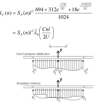
The first correction that does not give exact results because the nodal force resulting from wind pres-sures does not result from prespres-sures on one element only but on contiguous elements. Figure 6 illustrates the problem for a straight structure. In this case, the force F results from the pressures applied on two elements.

In the simplified method, the wind pressures are supposed to be constant on half of elements. In this case, the resulting nodal force can be computed by (see Equ. 10):

(

3 1 26 2 3 3

)

32 p p p

l

F = + + (18)

and then the PSD of the nodal force is given by:

( ) 1024 18 312 694 ) ( ) ( 2 2 2 2 U l Cn U Cnl P F e e l n S n S − − + + = ⎟ ⎠ ⎞ ⎜ ⎝ ⎛ = U Cnl l n S_P 2 ˆ ) ( 2λ₀ (19) 3 p₁ 2 F F₂ F₁(l) F₂(l) F₁(r) (r) F p p

Exact pressure distribution

Simplified method

x y

Fig 6: Illustration of the second correction

On the other hand, if the exact pressure distribution is taken into account, we can see that the nodal force is expressed by:

∫

+ = + =_F l _F r l _L _x _p _x _dx l _L _y _p _y _dy F 0 0 ) ( 1 ) ( 2 ( ) ( ) ( ) ( ) (20)

This relation gives a better approximation of the PSD of the nodal force. It can be obtained by sidering combinations of pressures along both con-tiguous finite elements:

⎟ ⎠ ⎞ ⎜ ⎝ ⎛ = U Cnl l n S n S_F _P 2 ) ( ) ( 0 2λ (21) In this relation function λ₀ is used to represent the

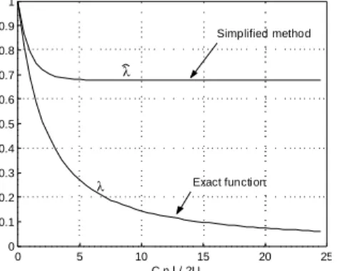
exact reduction of the nodal force resulting from the coherence in wind pressures. This relation should be compared to its approximate λ obtained with the ˆ₀ simplified method. These functions can be seen as an upgrade of the functions presented in the previous paragraph. Figure 7 gives a graphical representation of these new functions. The conclusions that can be

(5)

drawn from the observation of this figure are identi-cal to those formulated for figure 4.

0 5 10 15 20 25 0 0.1 0.2 0.3 0.4 0.5 0.6 0.7 0.8 0.9 1 C n l / 2U Simplified method Exact function λ λ

Fig. 7: Non dimensional functions representing the reduction of the nodal force resulting from wind pressures on two elements

The comparison of these two functions allows de-fining a new (and more precise) numerical admit-tance: ⎟ ⎠ ⎞ ⎜ ⎝ ⎛ ⎟ ⎠ ⎞ ⎜ ⎝ ⎛ = ⎟ ⎠ ⎞ ⎜ ⎝ ⎛ U Cnl U Cnl U Cnl 2 ˆ 2 2 0 0 0 λ λ χ (22)

Exactly as we did in the previous paragraph, this correction function could be used in order to correct the PSDM of the applied nodal forces.

This correction gives a better representation of the coherence field. Indeed, figure 8 represents the ratio between analytical and numerical analyses. We can see that the new “nodal correction” gives a better approximation of the generalized force in the first mode. W/O corr. Element corr. Nodal corr. 0 5 10 15 20 25 30 0 0.2 0.4 0.6 0.8 1 1.2 C n l /2 U

5.4 Third correction

Even if the second correction gives a better ap-proximation of the coherence field, it is however not perfect yet. The reason of this comes from the fact that the last result was obtained by correcting the whole PSDM (of nodal forces) by the same numeri-cal admittance.

Actually, this correction was valid for the diago-nal terms (the PSD of the nodal forces) since they have been computed in such a context; but, there is no reason to apply the same correction function to

off-diagonal terms (cross PSD’s between forces at different nodes). We will now show that these terms have to be corrected by different numerical admit-tances. These new functions can be computed by considering successively the cross-PSD’s obtained by the simplified method and by the exact one.

The developments must be realized for any “dis-tance” between the considered forces. Let us con-sider for instance that it is desired to compute the cross-PSD between forces acting k finite elements from each other (Fig. 9).

k.l

F2 F1

Fig. 9: Illustration of the third correction (k=2)

On one hand, in the simplified method, each of these two forces results from the evaluation of wind pressures at three points only (see § 5.3, Fig. 6). In the more general case, the cross-PSD between F1

and F2 is then expressed as a function of wind

pres-sures at six points of the structure. Let us also re-member that, in this method, the pressures are sup-posed to be constant on half of the finite elements. This formulation leads to a complex expression:

⎟ ⎠ ⎞ ⎜ ⎝ ⎛ = U Cnl l n S n S_F_F _P _k 2 ˆ ) ( ) ( 2 2 1 λ (23)

which is equivalent to Equ. 19, but for cross-PSD’s in this case. The new function λˆ_k introduced in this relation allows taking into account (in a limited way !) the force reduction resulting from the coherence of the wind along the structure.

On the other hand, the exact cross-PSD between forces acting at two different nodes can be ex-pressed. The developments are quite heavy and are therefore not presented here. They are based on the same reasoning than in the previous paragraph: an exact estimation of the forces (Equ. 20) must be considered for F1 and for F2 and then the cross-PSD

(cf Equ. 21) of these two values can be estimated. After some mathematical developments, this leads to: ⎟ ⎠ ⎞ ⎜ ⎝ ⎛ = U Cnl l n S n S_F_F _P _k 2 ) ( ) ( 2 2 1 λ (24)

where λ_k is now the exact function accounting for the reduction in wind forces. Note that expressions

k λˆ _and

k

λ reduce to λ and ˆ₀ λ₀ when unilateral PSD’s are considered. These functions can thus be seen as a generalization of the developments of the previous paragraph.

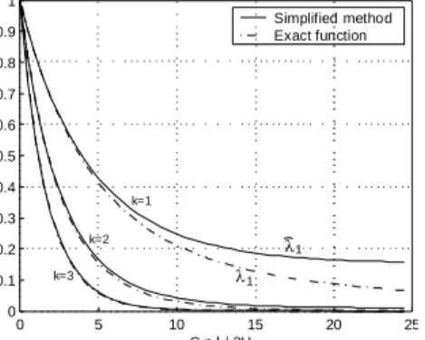
Figure 10 represents the new functions. Exactly as for unilateral PSD’s, it can be seen that the high frequency content is not well estimated with the

(6)

simplified method. This overestimation of the coher-ence between nodal forces comes from a bad ac-counting of the coherence of wind pressures along the structure. 0 5 10 15 20 25 0 0.1 0.2 0.3 0.4 0.5 0.6 0.7 0.8 0.9 1 C n l / 2U λ Simplified method Exact function k=2 1 λ1 k=3 k=1

Fig. 10: Non dimensional functions representing the reduction of the coherence between different nodal forces

These new functions can be used to define a new numerical admittance that is appropriated to the pair of forces that are considered. In this way, we can thus define numerical admittances for:

• unilateral PSD’s (k=0, Equ.22)

• forces that are one element away from each other (k=1);

• forces that are two elements away from each other (k=2);

• etc.

In the simple case of a straight structure whose elements have the same size, it is interesting to no-tice that numerical admittances for k≥2 are all the same. The analysis of the simple beam with these new numerical admittances can thus be realized by correcting the PSDM of the nodal force with differ-ent functions:

• one for diagonal elements;

• one for off-diagonal elements that are one element away from the diagonal

• and a last one for the rest of the matrix; On Figure 11, we have added a last comparison between analytical and numerical approaches. On this figure, it can be seen that using different nu-merical admittances for the different elements of the PSDM of the nodal forces can lead to very accurate results. W/O corr. Element corr. Nodal corr. Nodal corr. II 0 5 10 15 20 25 30 0 0.2 0.4 0.6 0.8 1 1.2 C n l /2 U

6 CONCLUSIONS

The coherence of wind forces must be taken care-fully into account in finite element developments. It is well known that the size of the finite elements should be small compared to the length scale of the wind turbulence (small Cnl 2/ U in the context of this paper).

Indeed, most finite elements formulations are simplified and do not allow a good representation of the high frequency content. As a first step, we have shown the limitation of such a simplified method. For typical analysis (mean wind velocity: U=25m/s, finite element size: l=15m, coherence coefficient:

C=8), it can be seen that the power spectral densities

of the forces are not well estimated above 1 Hz. In this paper we have presented a method allow-ing a better representation of the coherence in the wind field. This method could be applied in a more complex finite element in order to account for this coherence correctly, even with very large finite ele-ments.

For practical applications, it could be interesting to work with the simplified model and to use correc-tion funccorrec-tions in order to allow this better represen-tation. We have also presented these correction func-tions: the numerical admittances. As a last level of complexity, we have introduced numerical admit-tances that must be used to correct the different terms of the power spectral density matrix estab-lished with the simplified procedure.

These correction terms give a very good accuracy when the structure is straight and is represented with finite elements of equal length. For more complex structures (in shape), other admittance functions can be used. The method using numerical admittances can thus be applied in a wide range of applications. 7 ACKOWLEDGMENTS

The author would like to acknowledge the National Fund for Scientific Research.

8 REFERENCES

Clough, R. W. & Penzien, J. 1993.Dynamics of structures

(second edition). New York: Mc Graw-Hill : Civil

Engi-neering series.

Davenport, A.G. 1961. The application of statistical concepts to the wind loading of structures. Proceedings of the

In-stitue of Civil Engineers Vol. 19: p 449.

Denoël, V. 2003. Analysis of structures subjected to turbulent

wind loading. Graduation Work. Liège, Belgium :

Univer-sity of Liège (in French).

Dyrbye, C. & Hansen, S. O. 1997. Wind loads on structures. New York: Wiley & Sons.

Soize, C.& Krée, P. 1978. Mécanique aléatoire. Paris : Dunod Zienkiewicz, O. C. & Taylor, R. L. 2000. Finite Element