Lefebvre : Université du Québec à Montréal (UQAM) and Inter-university Centre on Risk, Economic Policies and Employment (CIRPEE). Address for correspondence : Pierre Lefebvre, Economics, UQAM, CP 8888, Succ. Centre-Ville, Montréal, QC, Canada H3C 3P8; Tel.: 514-987-3000 #8373; Fax: 514-987-8494
lefebvre.pierre@uqam.ca
Merrigan: UQAM and CIRPEE Verstraete: UQAM
The analysis is based on Statistics Canada’s National Longitudinal Survey on Children and Youth (NLSCY) restricted-access Micro data Files, which contain anonymized data collected in the NLSCY and are available at the Québec Inter-university Centre for Social Statistics (QICSS), one of the Canadian Research Data Centers network. All computations on these micro-data were prepared by the authors who assume the responsibility for the use and interpretation of these data. This research was funded by the Fonds québécois de la recherche sur la société et la culture. We would like to thank participants at the Canadian Economics Association Annual Meeting (Vancouver, June 2008) and the SCSE Annual Conference (Montebello, May 2008).
Cahier de recherche/Working Paper 08-22
The Effects of School Quality and Family Functioning on Youth Math
Scores : a Canadian Longitudinal Analysis
Pierre Lefebvre Philip Merrigan Matthieu Verstraete
Abstract:
This paper tries to disentangle the relative importance of family and school inputs on a child’s cognitive achievement as measured by her percentile score on a mathematics test. We replicate a study by Todd and Wolpin (2007) in the United States with Canadian data. In contrast to their work that uses state-level indicators of school quality we estimate our model with data from Statistics Canada’s National Longitudinal Survey of Children and Youth (NLSCY) which provides micro-level information on the family and school history of the child. The sample used for the analysis is based on the 7- to 15-year-old longitudinal children who have completed at least two consecutive math tests. As in Todd and Wolpin, we conclude that cognitive outcomes are determined by current and past family inputs. Contrary to them, who find no impact of school inputs, we find that the quality of schools has a positive impact on achievement in mathematics.
Keywords: Math scores, human capital, child development, school and family inputs,
panel data
1. Introduction
For several years a heated debate has raged on the effectiveness of the educational system at large. Hanushek (2003, 1997) provides an impressive summary of the results found in this area and concludes that no clear picture emerges as to the role of educational inputs for the performance of students, be they the teacher-pupil ratio, teacher education, or expenditure per pupil.
However, Krueger (2003) presents a slightly different picture of the meta-analyses conducted by Hanushek (1997, 2003). Giving equal weight to the studies the latter uses for his 1997 literature survey, Krueger remarks that: “[…] resources are systematically related to student achievement.” Referring to Tennessee’s Project STAR,1 Krueger emphasizes the importance of “sample size and strength of design” when analyzing the results of an educational experiment.
Webbink’s (2005) very thorough review of recent articles on the effects of school inputs on achievement underlines the endogeneity problem that has bedeviled many “traditional” studies. He presents recent methods such as randomized experiments and observational studies with credible IV estimators used to overcome this hurdle. In the “New Studies”, as he coins recent articles based on credible exogenous variations of the variable of interest (class size, school hours, school choice, etc.), he finds that: “[…] the range of findings is limited to significant or not.” Table A1, taken from Webbink’s review, clearly demonstrates this point. Recently, Todd and Wolpin (2007), with a very rich specification, find no impact of school inputs on the cognitive achievement (math and reading tests scores) with a panel of children living in the United States. Therefore, the evidence on the impact of school inputs remains mixed.
We replicate the Todd and Wolpin study with Canadian data. In contrast to Todd and Wolpin, who use state-level indicators of school inputs, the data used for this study provides micro-level information on school inputs. Our methodology is based on that of Todd and Wolpin (2003, 2007) and relies on the family and school history of the child.
The goal of this paper is to try to disentangle the relative importance of family functioning and school inputs on a child’s cognitive achievement as measured by her percentile score on a math test. The data used for the regressions are provided by Statistics Canada’s National Longitudinal Survey of Children and Youth (NLSCY) and the analysis is based on the 7- to
1 Tennessee’s Project STAR is “a large-scale, four-year, longitudinal, experimental study of reduced class size”
year-old longitudinal children who completed at least two consecutive math tests from one cycle of the survey to the next. The family input to which we refer throughout the analysis is the family functioning scale as provided by Statistics Canada.2 In order to be parsimonious, as is the case with the family functioning scale, and because a model with a separate variable for each school characteristic is prone to identification problems as school inputs are strongly correlated, we aggregate the continuous and discrete variables pertaining to school quality (available in the NLSCY cycles) into a single school index reflecting the quality of the school the child attends. A major difficulty encountered while constructing this index was the presence of missing values for the school quality indicators. Therefore, we perform two sets of regressions: one with a dummy variable in the specification when information on a school characteristic used to construct the school index is missing, and one with imputed values constructed following a multiple imputation method.
One of the main conclusions of Todd and Wolpin (2007) is the importance of including past as well as current values of school and family inputs in a regression of achievement scores on inputs. Additional recent empirical evidence summarized and provided in Cunha et al. (2006) suggests that a child’s learning process is a cumulative process, and that today’s cognitive outcomes are determined by present and past family and school inputs. Our estimates reinforce this conclusion but, in contrast to Todd and Wolpin (2007), we find that the quality of schools has a positive impact on performance in math. For certain credible specifications, we find that if a child moved from a perfectly functional to a permanently dysfunctional family and from a mediocre to an excellent school environment, ceteris paribus, an excellent school would almost entirely mitigate the adverse effects of a completely dysfunctional family.
The paper is structured as follows. Section 2 describes and discusses important issues for this area of research by emphasizing some of the main results of the Program for International Student Assessment (PISA). This provides a useful context against which our results can be analysed. Section 2 also reviews some of the latest findings in the field of educational research in the economic literature. Section 3 briefly presents the Todd and Wolpin (2007) modeling approach that is used in the present paper. Section 4 describes the data set, the variables retained
2
As stated in the NLSCY’s user guide for the first survey (1994-1995): “This scale was administered to the Person Most Knowledgeable (PMK) of the child, generally the child’s mother, or to the spouse/partner on the Parent Questionnaire, and measures how family members relate to each to other.” More precisely: “Questions related to family functioning were developed by researchers at the Chedoke-McMaster Hospital of McMaster University and have been used widely both in Canada and abroad. This scale is used to measure various aspects of family functioning, e.g. problem solving, communications, roles, affective involvement, affective responsiveness and behaviour control.”
for the analysis, the imputation method used for the missing school inputs and the construction of the school index. Section 5 presents and discusses the regression results. Section 6 concludes the paper.
2. Main issues and literature review
A convincing piece of evidence that characteristics of the school system do play a role in educational achievement, and within country of schools themselves (as well as parents and home environment), are the results from the Program for International Student Assessment (PISA), conducted regularly by the Organisation for Economic Co-operation and Development (OECD, 2001, 2004, 2007). From PISA’s 2003 results on math scores3 for the 26 countries that participated, three important points stand out from the empirical evidence.
First, within countries, some countries are observed with both a high average performance and small disparities between students’ proficiency levels as measured by the differences between the 75 and 25 percentiles or the variance of the scores. The wide variation in overall student performances is evidently correlated with the characteristics of the country’s school system, but not necessarily with the nature of the school system. Take Italy for example. It is a country with a low average performance and with a highly centralized educational system. However, the results show large territorial differences in student performance. By contrast, Canada, a country with mean performances significantly above the OECD average, has a much decentralized educational system (entirely under the jurisdiction of the 10 provinces) with both French and English language school systems in 5 provinces.4 The proportion of Canadian students at the very low proficiency Level 1 or below in math was approximately half the proportion of the OECD average (10% versus 21% respectively). In contrast, a significantly higher proportion of Canadian students performed at Level 5 or above in math. For those proficiency levels, the OECD average was approximately 15%, five percentage points lower than Canada’s average. However, the average performance per province based on the combined math
3 Mathematics achievement was divided into six proficiency levels representing a group of tasks of increasing
difficulty, and four mathematics sub-domains (space and shape, change and relationships, quantity, and uncertainty) as well as problem-solving skills.
4 The Canadian sample of students in both PISA 2000 and 2003 is one of the largest, only Mexico has similar
samples. In the United States for PISA 2003, approximately 5,500 students from 262 schools were tested. In Canada, approximately 30,000 15-year-old students from more than 1,000 schools participated in PISA 2000 and 2003 in order to collect information at the provincial level and to allow for estimates for both official language groups.
and variance of the scores did not establish a clear relationship for the rank performance of provinces.
Second, parents play a capital role in how students learn. Aside from being actively involved in their children’s education, parents provide a home environment that impacts learning because they are responsible for the educational resources available in the home. In PISA’s Surveys, parental education and occupation are the two major components of the socio-economic status (SES) of a student. The difference in average performance between students whose parents have a university degree versus high school or less education corresponds to about two-thirds of a proficiency level. These results suggest a positive relationship between the educational level achieved by parents and their child’s performance in math.
Third, schools play an important role in moderating the effects of individual SES.5 Canadian results based on the PISA’s survey (Bussière et al., 2004) show that when students have similar socioeconomic backgrounds, they tend to perform better, on average, in schools with higher average SES.6 This tendency suggests that students are not only affected by the socioeconomic circumstances of their own parents, but by those of their peers as well. Furthermore, students tend to perform better when they attend schools with students from high SES backgrounds, regardless of their own family’ SES.
The results of the PISA surveys raise two issues. First, a sizeable proportion of 15-year-olds appear to be not well prepared to meet the challenges of today's knowledge societies. The learning institutions at large display some difficulties producing a skilled and educated workforce. Second, because performance test scores are strongly correlated to labor market outcomes, disparities in achievement test scores are conducive to inequalities in labor market outcomes such as earnings. We know, for example, that individuals more proficient in math earn higher wages later in life (Rose and Betts 2005) and more generally, that cognitive skills are important determinants of educational attainment and earnings (Murname, Willett and Levy 1995; Neal and Johnson 1996; Cameron and Heckman 1998).7
If one restricts attention to the United States, a large part of the educational research literature has focused on “racial” test score gaps, mainly between White and Black children, and on the
5 There is no teacher survey in PISA’s Surveys unlike other educational assessments, so good teacher data is lacking. 6 After controlling for individual socioeconomic backgrounds and when schools are grouped into lowest, middle, and
highest thirds of average SES and for the typical range (25th to 75th percentiles) of mathematics scores.
7 Recent studies show that non-cognitive skills also play an important role in labour market outcomes (in the
determination of earnings and educational attainment). Although non-cognitive skills are more difficult to measure, they seem more malleable over the life cycle (Heckman, Stixrud and Urzua 2006; Cunha and Heckman 2007).
effects of “premarket factors” such as endowed ability, family background and structure, schools and other environmental influences (Cameron and Heckman 2001; Carneiro et al., 2006; Cunha and Heckman 2007; Todd and Wolpin 2007; Fryer and Levitt 2004, 2005; Murnane et al., 2006).
Fryer and Levitt’s (2004) preferred hypothesis for the mechanism driving the divergent trajectories of Black and White children is that African American children attend schools of lower quality. However, with more data at hand (i.e. for first and third grade children) and following tests of the following hypotheses: 1) African American children lose ground because they attend low-quality schools; 2) the importance of parental/environmental inputs grows as children age; 3) the type of material tested changed to the detriment of Blacks; Fryer and Levitt (2005) conclude that “The explanation as why Blacks are losing ground proves elusive.”
Todd and Wolpin (2007) use three databases8 to estimate models of cognitive achievement based on the full family and school history of the child. Their goal is to find the model that best predicts “racial” test score gaps. In doing so, they uncover empirical evidence which shows that present and past inputs matter for a child’s current achievement. They also emphasize the importance to control for endowed ability effects (e.g. child fixed-effects) in the estimation of education production functions in order to allow “input choices to be endogeneous with respect to unobserved endowments.” Their schooling variables (pupil-teacher ratio, teacher salary) are found to have no impact on the child’s development. However, these variables are state-level indicators (means). Their principal explanations for the observed “racial” test score gaps are that they are the result of differences in the mother’s “ability”, as measured by the Armed Forces Qualifying Test (AFQT), followed by those in home inputs. It should be noted that the home inputs used in their estimations are actually “home scales” derived from a summation of dichotomized items that change as the child ages.9
Cunha and Heckman (2007) underline the importance of non-cognitive skills for many personal outcomes such as wages, schooling, and teenage pregnancy. They also stress that it is capital to make a distinction between the different stages of development when analyzing the determinants of skills be they cognitive or non-cognitive. Many of the family and school inputs
8 The 1979 National Longitudinal Survey of Youth-Child Supplement (NLSY79-CS) for information on the children
born to women respondents of the NLSY79, home inputs and maternal characteristics; the Common Core Data (CCD) for pupil/teacher ratios at the state-level and county-level; and for teacher salaries data from the American Federation of Teachers from 1984 to 2001; the latter two are considered as school inputs.
9 The home scale provided in the public use files is considered a measure of the time and goods provided in the
home. The items are, for example, the number of books for children; musical instruments, hobbies, and special lessons (sports, arts); attending museums, musical and theatrical performances; daily newspapers, watching and discussing TV programs with the child; quality of the house.
used for the successful development of a child evolve as the child ages. In our view, the fact that Cunha and Heckman stress the distinction to be made between different developmental periods reinforces the case for the cumulative models estimated in this paper.10
As is clear in Table A1, borrowed from Webbink’s review of the literature on educational research, many school factors can have a positive impact on a pupil’s results: class size, performance incentives, peers in school, etc. Still, Table A1 of the results tends to suggest that teacher “quality”, as measured by training/acquisition of teachers, has no impact on student’s performance.
However, more recent studies have exploited the availability of detailed micro-level data on all teachers and students over many periods within states, or school districts, or cities, and the education production function framework, to explore in more details and with far more confidence than had been possible in previous studies the relationship between teacher characteristics and student test scores. Their results all support that teachers can and do make a positive difference on student performances, even if these variations are not strongly related to the teachers’ observable qualifications (Aaronson, Barrow and Sander 2007; Koedel and Betts 2007; Hanushek et al., 2005; Rivkin et al., 2005; Hanushek and Rivkin, 2006; Rivkin et al., 200511; Clotfelter, Ladd and Vigdor 2005, 2007; Rockoff 2004). As will become clear in section 4, the school index used in the present paper which is our measure of school quality relates to the whole school environment and not to the quality of teachers in particular.
3. Conceptual Framework and Econometric Approach
The empirical literature in the educational field has to deal mainly with two types of econometric problems. The first type relates to the shortcomings of data sets that are available on the academic achievement of children, family, child and school history. The second type pertains to the lack of a unified conceptual framework to analyze the data. Todd and Wolpin’s (2007) methodology to study the “racial” test score gap draws on their previous work (Todd and Wolpin 2003) and provides such a framework.12
10 Although the variables that compose our school index and the family functioning scale do not change over time. 11 A later study by this same group (with O’Brien 2005) verifies the importance of teacher quality in a specific Texas
school district using data linking students and teachers at the classroom level.
12 Todd and Wolpin (2007) state their approach: “[…] builds on Boardman and Murname (1979) who where the first
Among economists, one of the most popular approaches for the analysis of the effect of school quality on students’ achievement is the education production function. Todd and Wolpin (2007, 2003) explore in great details the underlying hypotheses of such education production functions in order to give causal interpretations of the key parameters of interest.
In order to estimate the causal impacts of the child’s family and school history on her math percentile score, we use Todd and Wolpin’s (2007) cumulative specification with child fixed effects.13 Let T be child’s i percentile math score at age a; ia Xia,Xia−2 ,..., the family functioning
score at age a, a-2, ..., a-n;14 Yia,Yia−2 ,...the values of the school index; Zia,Zia−2 ,...other observed
family and school characteristics; μi0 the child’s endowment; and e the residual. ia Econometrically, the cumulative model that is estimated using the NLSCY data is:
ia a i a i ia ia k is ia ia a i ia ia ia e Z Z Z Y Y Y X X X T + + + + + + + + + + + + + = − − − γ μ δ δ δ β β β α α α 0 0 2 2 1 2 2 1 0 2 2 1 ... ... ... (1) As our goal is to try to disentangle the relative contributions of the family’s and of the school’s characteristics on the child’s math performance we solely focus our presentation of the results (presented in Table 6) on theα1,α2,...αa andβ1,β2,...βk parameters, with s being the age children start in school. The estimates of the preceding cumulative model by a child fixed-effects estimation method are causal/consistent if the three following hypotheses are verified (see Todd and Wolpin 2007 for a more elaborate discussion). First, the effect of the child’s endowment does not vary through time or, said differently, with the child’s age. Second, and this is probably the weakest point of this modeling technique, prior results to the math test (eia−1) do not affect
present parenting practices (X ) or the choice of the child’s present schooling environment ia
(Y ). Third, omitted inputs must be constant over time. ia
Since the math test is first taken when the child is at least 7,15 we have no information on the children’s school environments prior to that age. Moreover, for the children who pass the test in
13 We were not able to estimate cumulative specifications with school fixed-effects as the NLSCY’s coding of the
children’s schools ID varies from one survey to the other. The sole purpose of the schools ID variable is to identify the children who are in the same school for a given survey. We were also not able to estimate sibling fixed-effects models because there were too few observations.
14 Since the NLSCY data is collected biennially the “normal” change in age for a child between two surveys is 2
years. Hence, in almost all cases, n is equal to two. However, from one survey to the other, the change in age of some children can be one or three years because the survey in conducted over two years (in the autumn and in winter-spring). These “outlier” cases are taken into account when constructing the lagged values of the family functioning scale and of the school index.
15 In fact the minimum age at which the test is first passed in the NLSCY is 6. But there were so few observations of
the first NLSCY cycle (1994-1995; children aged 7 to 11) we also have no information on their prior home environments.16 Because of this, we cannot observe the same number of lags for all children. Therefore we interact the lagged term with a dummy variable, as in Todd and Wolpin, indicating whether the lag is observed or not for the child. This depends on the age of the child and cycle of the NLSCY.
Two specification tests are conducted. The first consists of jointly testing the significance of the current and lagged key parameters of interest which are the coefficients of the family functioning scale and of the school index. The second is a Hausman test of the equality between these key coefficients obtained from the estimated child fixed-effects model, and of those resulting from a random-effects estimation.
4. Data
The data used for our regression analysis are provided by Statistics Canada’s National Longitudinal Survey of Children and Youth (NLSCY) which is a probability survey designed to provide information about children and youth in Canada. The survey covers a comprehensive range of topics including childcare, information on the physical and intellectual development of children, their behavior as well as data on their social environment (family, friends, schools and communities, family income). The NLSCY began in 1994-1995 and data collection occurs biennially. The unit of analysis for the NLSCY is the child or youth. Information for each selected child between 0 and 17 years of age and for her family is provided by the Person Most Knowledgeable about the child (PMK) who then conveys information about herself and her spouse/partner. The PMK is usually the child’s mother (in more than 90% of the cases), but it can also be the father, a step-parent or an adoptive parent who lives in the same dwelling.
In 1994-1995, a sample of children aged 0 to 11 was selected in each of the 10 provinces. Responding children (22,831) made up the first longitudinal sample. Then, in 1996-1997, to reduce the response burden on families with several eligible children, the number of children selected was limited to two per family. Therefore, some children were dropped from the sample (16,903 children remained in the longitudinal sample in the 2nd cycle of the survey) so that not all children from the first longitudinal sample (1994-1995 NLSCY survey) can be used for the estimations described in Table 6. Moreover, since the natural age progression of a child between
cycles of the survey is two years, only children aged at least 3 in the first cycle were retained in our database. A child aged 3 in the 1st cycle with a “normal” age progression of two years between surveys will be 5 in the 2nd cycle, 7 in the 3rd and 9 in the 4th, the last NLSCY cycle we use because information about the school the child attends is unavailable for the two last cycles of the survey (cycles 5 and 6). Such a child should be observed with only two scores because the first math test is taken at age 7. Older children in cycle 1 can be observed with more than two scores. We use data on children aged 7 to 15 with at least two consecutive test scores in math. Test scores
The CAT/2 test is a shorter version of the Mathematics Computation Test taken from the
Canadian Achievement Tests, 2nd edition.17 The CAT/2 is designed to measure basic competences
in math (addition, subtraction, multiplication and division on integers, etc.). The test is administered to children who were enrolled at least in the second grade.
The master files include both the CAT/2-raw and –standardized scores. The raw score is simply the number of correct answers in the test. The difficulty of the test varies with the school grade of the child. Statistics Canada standardizes the raw scores using a sample of Canadian children from the ten provinces which is called the normative sample. This sample was chosen by the Canadian Testing Center. The standardized scores are obtained using sub-samples (by school grade) of the normative sample.
A significant proportion (approximately 35%) of children in grade two obtained a perfect score when they passed the tests in 1994-1995 (1st NLSCY cycle). Therefore subsequent cycles added more versions of the tests. These added versions of the tests were still based on the school grades of children but with a clearer distinction made between school grades. For example, in 1994-1995 (cycle 1), children in the 2nd and 3rd grade (7- and 8-year-olds) took the level 2 test. Two years later, 2nd grade children (7-year-olds) took the level 2 test whereas 3rd grade children (8-year-olds) passed the level 3 test.
Since the mean value (and the range) of the CAT/2 standardized scores increases as children grow older (Table 1.A), it would be difficult to interpret the econometric results based on such scores. For example, in 1994-1995, 7-year-olds’ mean CAT/2 score is 319 whereas that of
17 The test was administered by the child’s teacher once the PMK of the child had given her consent. Since cycle4 of
the NLSCY, in order to minimize the time dedicated by teachers to the survey and to avoid disturbing class activities at the end of the school year, the math test is administered at the home of the child rather than in school.
year-olds’ is 420. Therefore, the Hazen method is applied to calculate another dependent variable for math achievement, percentile scores based on the standardized scores18
Family functioning and school inputs
Throughout the analysis both family and school characteristics are incorporated as regressors. The NLSCY data sets do not have items that permit the construction of “home scales” nor of the mother’s “ability” as in the NLCY79-CS in the Unites States.19
The family input variable used in the analyses is the family functioning scale provided by Statistics Canada.20 This scale is derived by summing up the answers to questions such as: “In our family, we feel accepted as we are” or, “Our family has some difficulties in making decisions”. As the NLSCY’s user guide for the 1st cycle (1994-1995) states: “This scale is aimed at providing a global assessment of family functioning and an indication of the quality of the relationships between parents or partners.” The more dysfunctional the family is the more the scale increases. The family functioning scale varies from 0 to 36.21
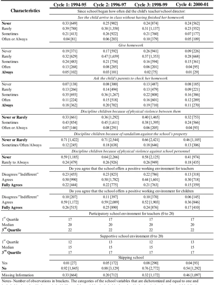
The school variables are divided into two categories: the continuous and the discrete variables. The continuous category regroups the following school inputs: the School’s Participatory Environment for Teachers and the School’s Supportive Environment. The discrete category contains the following school inputs: the Age Class of the Child’s Teacher;22 the Gender of the Child’s Teacher; the frequency with which the child’s teacher/director is forced to discipline the pupils because of: 1) Physical Violence Between Children; 2) Vandalism Against the School’s Property; 3) Physical Violence Against School Personnel; the extent to which the school provides a: 1) Positive Working Environment for Teachers; 2) Positive Working Environment for Pupils; the frequency with which the teacher: 1) Gives Homework; 2) Asks the Child’s Parents to Check her Homework; 3) Observes that the Child Arrived in Class with Unfinished Homework; and 4) Observes whether the Child Skipped School Without Permission.
Because of missing values and collinearity problems with the school variables, the impact of a school’s environment on a child’s cognitive development is synthetically assessed with a school
18http://www.stata.com/support/faqs/stat/pcrank.html The percentile scores are always calculated with regard to the
level of the test the child passed and for each cycle of the NLSCY used.
19 Items such as reading to a preschool child or hobbies and sport or musical activities practiced by a child are
available in some cycles of the survey but are not collected systematically for each cycle.
20 Other parenting scales variables (such as positive reaction, ineffective, consistent or rational parenting style) were
available but only for children aged 2 to 11. Hence the specification including three lags of the school index became impossible to implement because the children were not followed over a sufficient period of time in school.
21 In our sample the family functioning scale ranges from 0 to 33 (Table 2.B).
22 The Age Class of the Child’s Teacher is the only proxy available in the NLSCY to measure a teacher’s experience
index. This school index is based upon all the school inputs shown in the first panel of Table 5 except the Missing Information variable which gives us the proportion of children for which information is lacking on at least one of the variables composing the school index. The two continuous school variables (School’s Participatory and Supportive Environments) are dichotomized according to the following rule: a value of one is given if the score belongs to the last quartile of the distribution and zero otherwise. The discrete school variables are also dichotomized based on the a priori positive effect a particular category of the variable would exert on a child’s development. For example, a dummy variable is equal to one if the answer to the following question: “Do you agree that the school offers a positive working environment for pupils” is: “Fully Agrees”. Finally, the school index is the sum of the dichotomized categories of the school variables that compose it (see first panel of Table 5 where the categories corresponding to a value of 1 for the construction of the index are displayed in bold).
The main difficulty encountered when using the NLSCY’s data on school inputs is the presence of missing values, especially for the last cycle used (2000-2001). As one can observe from the Missing Information variable (bottom of the first panel of Table 5), the proportion of missing data on school variables varies between 20% and 46%. Due to the large number of missing values, one set of analyses is conducted with imputed values.
To detect for statistically significant differences in the characteristics of children with and without missing values before imputing, Wilcoxon two-sided tests (Table A.2) are performed by cycle of the NLSCY for each variable used in the procedure used to impute values. Based on the results of these tests, there are few differences between the two groups of children. Along most dimensions (e.g. family composition, PMK’s age at birth or education) the two groups of children share the same mean values.23 However there are significant differences such as those for income, city size, and school type, in cycle 4. Nonetheless, these test results provide support for the hypothesis that the missing data on school inputs are Missing At Random (MAR).24
Assuming the NLSCY’s data on school inputs are MAR, a multiple imputation Markov Chain Monte Carlo (MCMC) method is used to impute the missing values of the school variables composing the school index, as well as the gender and age class of the child’s teacher.25 Each
23 The observed differences apply mostly to the proportion of children with and without missing information within
different age groups or provinces.
24 The usual definition of Missing At Random is that the missing data for a variable Y are Missing at Random if the
probability of missing data on Y is unrelated to the value of Y, after controlling for other variables in the analysis.
25 The MI procedure with the MCMC option from the SAS© software was used to “fill” the missing values of the
imputation is done on a cycle by cycle basis. The MCMC method assumes the data are generated by a multivariate normal distribution. Each missing value is imputed ten times with, each time, a bootstrap re-sampling based on 90% of the entire sample. Re-sampling entails greater variability for the initial estimates that provide different starting values for the MCMC process.
Descriptive statistics
Table 1.A presents the mean standardized test score available in the data sets. Mean scores increase with children’s age and therefore with overall cognitive skills. Standard deviations are larger as children are older, indicating that gaps in achievement are greater. As explained before, these scores were transformed in percentile scores for regression analysis (Table 1.B). A percentile score is a relative measure of performance and, as explained earlier, a more appropriate means to assess the impact of a child’s family and school environments over time. Table 2.A presents the school index without (a) and with (b) imputation. The distributions of the index are rather large (0 to 11) and approximately normal. In the case of observed values (a), there is a large number (3,645) of missing values for the school index. Table 2.B presents the distribution of the family functioning scale showing that it is substantially skewed to the left. Table 3.A shows the mean of the school index by age and cycle for children without missing values in the school variables that compose the school index. Table 3.A suggests that school quality is higher in grade school when children are less than 12. The school index after imputation (Table 3.B) exhibits the same pattern between grade and secondary school. The imputed mean values by age and cycle are also systematically lower than the mean “observed” values, which could mean that the latter were observed in better school environments on average. Table 3.C presents the mean of the family functioning scale by age and cycle and suggests that differences in family functioning are small across ages and cycles.
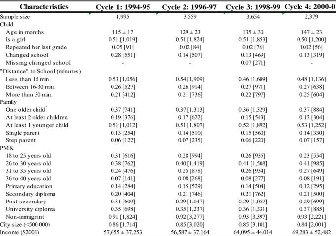
Table 4 presents the sample’s characteristics (children, families, and a few school variables). The increase of a child’s mean age in months between cycles ranges from 6 to 14 months. The immense majority (more than 90%) of children has a PMK born in Canada and roughly 15% of them live in a single parent family. Approximately 40% of children are born to a PMK aged 26 to 30 at the time of birth and roughly 50% are born to a PMK aged 18 to 25 or 31 to 35 at the time of birth. More than a third of PMKs are university educated and a little less than a third received a post-secondary education. More than half of the children have a younger sibling and 37% have a same age or only one older sibling. A large majority of children (84-86%) live in a city with less than 500,000 inhabitants. The real total family income (Can$2001) increases quite sizably
over the period of study, from about $58,000 to $69,000, as does its dispersion, from about $37,000 to $54,000. Roughly three quarter of the children live close to their school (30 min. or less commuting time). Very few children repeat a grade (2-5%) and, except for the first cycle (28%), a little more than one in ten children change school for a reason other than natural progression.
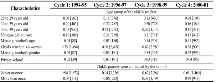
As the first panel of Table 5 displays, between 24% and 33% of children arrive in school with their homework always finished. The proportion of teachers that always give homework declines from 5% in the first cycle to 1% in the last. However, as we already noted, the proportion of missing values for school inputs is largest in the 4th cycle. The proportion of teachers that ask parents to always check their children’s homework remains stable at around 20%, except for the last cycle where it falls to 11%. Generally, a third to more than half of children evolves in a school environment where physical violence and degradation of school property is almost inexistent. More than half of the teachers are satisfied with their working environment and agree that their school offers a positive working environment for children. The distributions of the continuous school variables (School’s Participatory and Supportive Environments) are very stable throughout the cycles. The second panel of Table 5 shows that the majority of teachers in the sample belong to the 40 to 49 years old age class, except for the last cycle where there are a considerable number of missing values for this variable. The proportion of teachers belonging to the 30 to 39 years old or 50 years old or more age classes is roughly stable at approximately 20% each. Excluding the last cycle it is interesting to note that, as the children age, the proportion being taught by women tends to decline while the proportion that skips class without permission tends to increase. Finally, very few children attend a private school (2-4%) while the proportion of children whose parents are contacted more than once by the school tends to increase as the children age.
5. Econometric results
We conduct two sets of regression analyses, one with observed values (adding missing value dummy variables) and one with imputed values. In the regression analyses using the observed data the missing values of the school index are set to zero and we include the dummy variable Missing Information (on school inputs composing the school index, bottom of the first panel of Table 5) in the specification.
As the variance parameter resulting from the child fixed-effects (FE) estimation does not take into account the implicit estimation of the FE, we correct its number of degrees of freedom to obtain the correct variance-covariance matrix. In order to estimate a random-effects (RE) model,
we first estimate FE and Between models from which 2 2
2 1 e i e i Tσ σ σ θ μ + − = is derived, where T is i
the number of cycles child i is observed, 2
e
σ is the variance of the time-varying random error term and 2
μ
σ is the variance of the random effect.26 Finally, we use the algebra developed to aggregate the parameters obtained from the estimations using the different imputed data sets.27
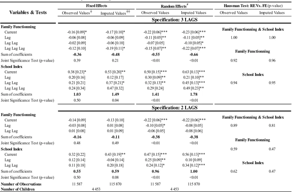
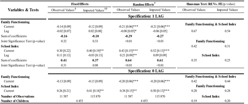
Table 6 presents the results from the regression of equation (1) with observed values and with imputed values respectively. Specifications differ according to the number of lags taken into account. We start our discussion with the specification that includes three lags (top panel of Table 6) for both school quality and family functioning scales. For the FE and RE models respectively, the cumulative effects (i.e. the sum of coefficients) of the family functioning scale estimated on the observed data with missing value dummy variables are -0.36 and -0.55 whereas they are -0.48 and -0.66 with the imputed data. For the school index, the cumulative effects are respectively, for the FE and RE models, 1.03 and 1.41 with missing value dummies and 1.49 and 1.78 with imputed data.
For both the observed and imputed data, the FE and RE parameter estimates of the school index and of the family functioning scale are quite similar. However the FE parameter estimates are systematically lower than those of the RE procedure which translates into estimated cumulative effects that are approximately 20% to 50% smaller for the FE specifications. This variation of cumulative effects is more pronounced for the family functioning scale. This means that the family functioning scale is more strongly correlated to unobserved fixed effects than the school index. There could be more within variation for the school index as it is probably more common for children to experience changes in schools than in families, particularly because of
26 T e K n Between SSR ˆ2 2 ˆμ σ σ − − = , where
∑
= iTi nT , n is the number of children in our sample, K the number of parameters in the between estimation, and 2ˆ
e
σ the variance of the FE estimation.
27http://www.stat.psu.edu/~jls/mifaq.html: For a description of the method used to combine the results across the
the change from elementary to high school, or due to moving from one district to another, or simply because of a change in principal or additional school funding.
In terms of the lag structure of the effects, for both variables (school index and family functioning), the current effect dominates. However, for the school index, the coefficients for the second and third lags are generally larger than for the first lag which at first glance could seem counterintuitive. Given that each cycle of the survey is separated by two years, the second and third lags are observed in grade school. Therefore, in some sense we are capturing quality of grade school effects with the last lagged school index variables. For family functioning, the coefficient of the first and second lags are smaller than for the current effect, however the third lag has a larger impact than lags one and two. Again, this is capturing effects when the child is much younger. Therefore, there could be an interaction effect between family functioning and the age of the child, just as Cunha and Heckman (2006) show that some periods are more critical for development and occur generally at a young age.
Three Hausman tests were performed for each specification in both data sets. The first compares family functioning and school index coefficients (current and lagged) of the FE and RE models. The second and third test the family functioning and school index coefficients separately. In all cases, we cannot reject the RE model. Three out of the four estimated family functioning coefficients for the RE model and observed data with missing value dummies are significant. With the imputed data, all parameters are found to be significantly different from 0. This is also true for the schooling coefficients. Therefore, we find considerable support for the 3 lag RE model. Hence, there is a credible statistical case to make that a long stay in a good quality school or in a well functioning family can lead to appreciable improvement in mathematics.
These effects are substantial and demonstrate that very good schools can make a positive difference for children and youths. Given the more conservative estimates of the FE model with observed data, gaining permanent access to a high quality school with an 11 score, the maximum of the school index, instead of attending a mediocre school with a score of 0, the minimum of the school index, entails an approximate 11 rank increase in the math test. For the family function scale the same exercise (moving from 0 to 33) will produce a decrease of almost 12 percentile points.
The model provides additional evidence to support the Todd and Wolpin assertion that lagged values of input variables in a cognitive achievement production function may lead to a much different assessment of the explanatory power of the inputs. The estimates of the coefficient on
the school index when only the current value is included range from .26 to .50 (Tables 6, bottom panel), which is approximately one third the size of the sum of the 4 coefficients in the model with three lags. The same can be said of the family functioning scale. For example, the RE model with missing value dummies with no lagged values produces a coefficient of -0.20 on the current value of the functioning scale whereas the sum of the coefficients is -0.55 for the three lag model.
Looking at estimates with different lag structures for the school index, the addition of a second lag is crucial for the results. A model with a single lag will seriously reduce the estimated effects of school quality on math scores. As for the family functioning scale, the third lag is crucial.
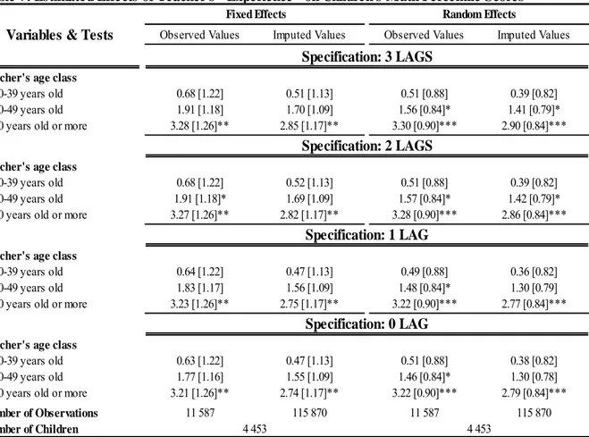
Finally, Table 7 presents results that concern the age class of the child’s teacher which is good a proxy for experience. For the regression, we fix the teacher’s age class of reference at the 20-29 years old category. We find that the effects of teacher’s age are non linear and increasing with the age class of the teacher. However it seems that, as the teacher ages, the positive effects of experience tend to increase at a slower rate. The effect of having a teacher in the “50 years old or more” age range is relatively large compared to a teacher in the 20-29 age group as it is estimated to be approximately three percentile ranks. Finally, the small variations of the age class coefficients across types of regressions (FE and RE) suggest that these variables are exogenous.
6. Concluding remarks
A model with a separate variable for each school characteristic is prone to identification problems for school input effects as they are strongly positively correlated. A single school index does not suffer from such a problem and captures many features of a school’s characteristics which, in our opinion, are important to a child’s development. More work should be done to construct better school indexes, but this first stab is promising. A more structural approach modeling the school quality indicators as a function of latent variables that would affect math achievement would certainly lead to a richer set of explanations for a study of this kind.
The orders of magnitude of this paper’s results, as regards the cumulative effects of a school’s environments on a child’s math score, point towards the fact that the quality of a school does make a difference for a child’s development. The same is true of family functioning, but this is less surprising as family inputs have been shown in several papers to be of the utmost importance. Future work should seek to find proper instruments, possibly policy variation from one province to the next to verify if our results still hold under a different set of assumptions
concerning the relationship between our key explanatory variables and the error term. We also find relatively strong teacher age (a very good proxy for experience) effects on math achievement.
In conclusion, the availability of panel data, because of the importance of lags in the model and micro data on schools, because of the precision they provide for estimation, are crucial for a comprehensive understanding of the role schools and families can play for achievement in mathematics, a powerful predictor of future success in life.
References
Aaronson, Daniel, Lisa Barrow and William Sander. 2003. “Teachers and Student Achievement in the Chicago Public High Schools,” Federal Reserve Bank of Chicago, WP 02-28.
Boardman, E. and R. Murnane. 1979. “Using Panel Data to Improve Estimates of the Determinants of Educational Achievement,” Sociology of Education, 52 (March):113-121.
Bussière, P., F. Cartwright, T. Knighton and T. Rogers. 2004. “The performance of Canada’s youth in mathematics, reading, science and problem solving: first findings for Canadians aged 15,” Catalogue no. 81-590-XPE, www.pisa.gc.ca; www.statcan.ca.
Cameron, S. and J. Heckman. 2001. “The Dynamics of Educational Attainment for Black, Hispanic and White Males,” Journal of Political Economy, 109 (June): 455-499.
Cameron, S. and, J. Heckman. 1998. “Life Cycle Schooling and Dynamic Selection Bias: Models and Evidence for Five Cohorts of American Males,” Journal of Political Economy, 106 (April): 262-333. Clotfelter, Charles T., Helen F. Ladd, and Jacob L. Vigdor. 2005. “Who Teaches Whom? Race and the
Distribution of Novice Teachers,” Economics of Education Review 24 (August): 377–92.
———. 2006. “Teacher-Student Matching and the Assessment of Teacher Effectiveness,” Working Paper 11936. Cambridge, Mass.: National Bureau of Economic Research (January).
Cunha, F. and J. Heckman. 2007. “Formulating, Identifying and Estimating the Technology of Cognitive and Non-cognitive Skill Formation,” Manuscript, Dept. Econ., Univ. of Chicago. Forthcoming, Journal of Human Resources.
Cunha, Flavio and James Heckman. 2006. “Investing in our Young People,” Manuscript, Dept. Econ., paper Univ. of Chicago.
Cunha, Flavio, James J. Heckman, Lance Lochner, and Dimitriy V. Masterov. 2006. “Interpreting Evidence of Life Cycle Skill Formation.” In Handbook of the Economics of Education, edited by Eric Hanushek and Finis Welch. New York: Elsevier, vol. 1: 697-812.
Fryer, Ronald G., and Steven D. Levitt. 2005. “The Black-White Test Score Gap through Third Grade,” Working Paper 11049. Cambridge, Mass.: National Bureau of Economic Research (January).
Fryer, Ronald G., and Steven D. Levitt. 2004. “Understanding the Black-White Test Score Gap in the First Two Years of School.” Review of Economics and Statistics 86 (May): 447–64.
Koedel, Corey and Julian Betts. 2005. “Re-Examining the Role of Teacher Quality in the Educational Production Function,” UCSD Public Policy Institute of California.
Hansen, K. T., J. J. Heckman, and K. J. Mullen. 2004. “The Effect of Schooling and Ability on Achievement Test Scores,” Journal of Econometrics, 121 (July-August): 39-98.
Hanushek, Eric, and Steven Rivkin. 2006. “The Evolution of the Black-White Achievement Gap in Elementary and Middle Schools,” Paper presented at the American Economic Association Annual Meetings, Boston, Massachusetts, January 6–8.
Hanushek, Eric, John Kain, Daniel O’Brien and Steven Rivkin. 2005. “The Market for Teacher Quality,” NBER, WP 11154, 2005.
Hanushek, Eric. 2003. “The Failure of Input-based Schooling Policies”, Economic Journal, 113 (February): F64–98.
Hanushek, Eric. 1997. “Assessing the effects of school resources on student performance: an update”, Educational Evaluation and Policy Analysis, 19 (Summer): 141–64.
Hanushek, Eric. 1996. “Measuring Investment in Education,” The Journal of Economic Perspectives, 10 (Fall): 9-30.
Heckman, J., J. Stixrud and S. Urzua. 2006. “The Effects of Cognitive and Noncognitive Abilities on Labor Market Outcomes and Social Behavior,” NBER Working Paper 12006.
Krueger, Alan. 2003. “Economic Considerations and Class Size,”The Economic Journal, 113 (February): F34–F63.
Murname, Richard, J. Willet, Bub Kristenl, and Kathleen McCartney. 2006. “Understanding Trends in the Black-White Achievement Gaps during the First Years of School,” Brookings-Wharton Papers on Urban Affairs, 97-135.
Murnane, R. J. Willet, J. B., and Levy, F. 1995. “The Growing Importance of Cognitive Skills in Wage Determination,” Review of Economics and Statistics, 77 (May): 251-266.
Neal, D. and Johnson, W. 1996. “The Role of Pre-Market Factors in Black-white Wage Differences,” Journal of Political Economy, 104 (October): 869-895.
OECD. 2007. PISA 2006 Science Competencies for Tomorrow's World, The PISA homepage at www.pisa.oecd.org.
OECD. 2004. Learning for Tomorrow’s World – First results from PISA 2003, Paris. The PISA homepage at www.pisa.oecd.org.
OECD. 2001. Knowledge and Skills for Life: First Reults from the OECD Programme for International Student Assessment (PISA) 2000, Paris. The PISA homepage at www.pisa.oecd.org.
Rivkin, S., Eric Hanushek, and J. Kain. 2005. “Teachers, Schools, and Academic Achievement,” Econometrica 73 (March): 417-458.
Rockoff, Jonah. 2004. “The Impact of Individual Teachers on Student Achievement: Evidence from Panel Data,” American Economic Review, Papers and Proceedings, 94 (May): 247-252.
Rose, Heather and Julian R. Betts. 2004. “The Effect of High School Courses on Earnings,” Review of Economics and Statistics, 86 (May): 497-513.
Todd, Petra and Kenneth Wolpin. 2003. “On the Specification and Estimation of the Production Function for Cognitive Achievement,” Economic Journal, 113 (February): F3-F33.
Todd, Petra and Kenneth Wolpin. 2007. “The Production of cognitive Achievement in children: Home, School, and Racial Test Score Gaps,” Journal of Human Capital, 1 (Winter): 91-136.
Webbink, Dinand. 2005. “Causal Effects in Education,” Journal of Economic Surveys, 19 (September): 535-560.
Cycle 1: 1994-95 Cycle 2: 1996-97 Cycle 3: 1998-99 Cycle 4: 2000-01 319 (50) 316 (48) 299 (40) -[314] [331] [363] -358 (49) 373 (55) 351 (51) -[427] [436] [448] -420 (61) 419 (57) 398 (52) 386 (56) [391] [535] [390] [371] 471 (57) 453 (58) 435 (58) 421 (53) [444] [597] [559] [385] 498 (63) 490 (66) 462 (59) 452 (59) [419] [519] [361] [360] - 524 (66) 488 (64) 483 (63) - [610] [490] [369] - 554 (86) 523 (80) 516 (73) - [531] [300] [318] - - 602 (93) 574 (92) - - [438] [316] - - 628 (93) 591 (85) - - [305] [260]
Table 1.A: Mean Math Standardized Test Score by Age and Cycle
Mean Score (Standard Deviation) [Number of Observations]
Fifteen year olds
Age of Children
Seven year olds Eight year olds Nine year olds Ten year olds Eleven year olds Twelve year olds
Source: Author’s calculation from the cross-sectional micro-data sets of the NLSCY. Note-The test is a shorter version of the Mathematics Computation Test-CAT/2.
Thirteen year olds Fourteen year olds
Cycle 1: 1994-95 Cycle 2: 1996-97 Cycle 3: 1998-99 Cycle 4: 2000-01
38 (27) 49 (29) 50 (29) -[314] [331] [363] -57 (27) 51 (29) 50 (29) -[427] [436] [448] -42 (27) 50 (28) 51 (29) 50 (29) [391] [535] [390] [371] 59 (27) 50 (29) 50 (29) 50 (28) [444] [597] [559] [385] 51 (29) 51 (29) 50 (29) 51 (29) [419] [519] [361] [360] - 51 (28) 50 (29) 50 (29) - [610] [490] [369] - 49 (29) 49 (29) 50 (29) - [531] [300] [318] - - 48 (29) 50 (29) - - [438] [316] - - 52 (29) 49 (29) - - [305] [260]
Table 1.B: Mean Hazen Percentile Test Score by Age and Cycle
Age of Children Mean Score (Standard Deviation) [Number of Observations]
Seven year olds Eight year olds Nine year olds Ten year olds
Fifteen year olds Eleven year olds Twelve year olds Thirteen year olds Fourteen year olds
Note-The Hazen percentile scores are computed for each level of the test the child passed and for each cycle of the NLSCY used.
0 22 0.28 0.28 0 400 0.35 0.35 1 224 2.82 3.10 1 3,693 3.19 3.53 2 701 8.83 11.92 2 10,799 9.32 12.85 3 1,372 17.28 29.20 3 20,539 17.73 30.58 4 1,794 22.59 51.79 4 26,135 22.56 53.13 5 1,369 17.24 69.03 5 20,063 17.32 70.45 6 840 10.58 79.60 6 12,716 10.97 81.42 7 663 8.35 87.95 7 9,411 8.12 89.55 8 532 6.70 94.65 8 6,932 5.98 95.53 9 312 3.93 98.58 9 3,778 3.26 98.79 10 103 1.30 99.87 10 1,284 1.11 99.90 11 10 0.13 100.00 11 120 0.10 100.00
Notes-The higher the value of the school index the better is the child's school environement. In the case of Observed Values (a) there are 3,645 observations with missing values for the school index.
Table 2.A: Distribution of the School Index
Value of School Index
"Number" of
children Cell Percent
Cumulative Percent Value of
School Index
Number of
children Cell Percent
Cumulative Percent
(a) Observed Values (b) Imputed Values (10 imputations per child)
0 771 6.65 6.65 1 498 4.30 10.95 2 486 4.19 15.15 3 524 4.52 19.67 4 492 4.25 23.91 5 537 4.63 28.55 6 581 5.01 33.56 7 634 5.47 39.04 8 674 5.82 44.85 9 677 5.84 50.69 10 787 6.79 57.49 11 915 7.90 65.38 12 2,102 18.14 83.52 13 807 6.96 90.49 14 365 3.15 93.64 15 238 2.05 95.69 16 153 1.32 97.01 17 90 0.78 97.79 18 76 0.66 98.45 19 35 0.30 98.75 20 40 0.35 99.09 21 22 0.19 99.28 22 16 0.14 99.42 23 18 0.16 99.58 24 17 0.15 99.72 25 9 0.08 99.80 26 8 0.07 99.87 27 to 33 15 0.13 100.00
Notes-The higher the value of the family functionning scale the worst is the child's family environement. 155 observations were dropped because of missing values.
Table 2.B : Distribution of the Family Functionning Scale Observed Values
Value of the Family Scale
Number of
children Cell Percent
Cumulative Percent
Cycle 1: 1994-95 Cycle 2: 1996-97 Cycle 3: 1998-99 Cycle 4: 2000-01 5.14 (2.06) 5.03 (2.03) 5.18 (2.11) -[193] [228] [240] -4.92 (1.89) 4.79 (2.03) 4.91 (2.08) -[266] [357] [308] -4.81 (2.14) 4.74 (2.05) 4.93 (2.19) 5.34 (2.20) [257] [421] [302] [184] 4.65 (1.98) 4.67 (1.99) 4.86 (2.14) 5.14 (2.28) [320] [491] [395] [218] 4.74 (2.06) 4.63 (1.96) 4.71 (1.93) 4.97 (1.99) [295] [423] [261] [206] - 4.43 (2.05) 4.64 (2.11) 4.71 (2.02) - [496] [336] [203] - 4.21 (1.88) 4.53 (1.99) 4.70 (2.07) - [431] [187] [186] - - 4.56 (1.93) 4.39 (2.00) - - [273] [165] - - 4.62 (2.03) 4.63 (2.03) - - [180] [120]
Note- "Observed" in the sense that each of the variables included in the school index is not missing.
Table 3.A: Mean Value of "Observed" School Index by Age and Cycle
Age of Children Mean Value (Standard Deviation) [Number of Observations]
Seven year olds Eight year olds Nine year olds Ten year olds
Fifteen year olds Eleven year olds Twelve year olds Thirteen year olds Fourteen year olds
Cycle 1: 1994-95 Cycle 2: 1996-97 Cycle 3: 1998-99 Cycle 4: 2000-01
4.98 (2.03) 4.91 (2.06) 4.91 (2.05) -[3,140] [3,310] [3,630] -4.82 (1.97) 4.70 (2.02) 4.76 (2.08) -[4,270] [4,360] [4,480] -4.71 (2.08) 4.64 (2.03) 4.90 (2.14) 5.13 (2.05) [3,910] [5,350] [3,900] [3,710] 4.63 (1.99) 4.63 (1.94) 4.73 (2.07) 5.00 (2.10) [4,440] [5,970] [5,590] [3,850] 4.61 (2.02) 4.54 (1.95) 4.61 (1.96) 4.91 (1.92) [4,190] [5,190] [3,610] [3,600] - 4.37 (2.06) 4.41 (2.03) 4.59 (1.92) - [6,100] [4,900] [3,690] - 4.16 (1.87) 4.39 (1.97) 4.59 (1.96) - [5,310] [3,000] [3,180] - - 4.40 (1.90) 4.27 (1.90) - - [4,380] [3,160] - - 4.44 (1.92) 4.45 (1.89) - - [3,050] [2,600]
Table 3.B: Mean Value of Imputed School Index by Age and Cycle
Age of Children Mean Value (Standard Deviation) [Number of "Observations"]
Seven year olds Eight year olds Nine year olds Ten year olds
Fifteen year olds Eleven year olds Twelve year olds Thirteen year olds Fourteen year olds
Cycle 1: 1994-95 Cycle 2: 1996-97 Cycle 3: 1998-99 Cycle 4: 2000-01 7.89 (4.92) 7.70 (4.98) 8.68 (4.39) -[314] [331] [363] -8.56 (5.07) 8.26 (5.01) 8.07 (4.66) -[427] [436] [448] -8.71 (4.99) 8.18 (4.96) 8.23 (5.03) 9.08 (4.50) [391] [535] [390] [371] 8.30 (5.26) 8.19 (4.74) 8.69 (4.81) 8.65 (4.98) [444] [597] [559] [385] 8.39 (5.31) 8.54 (4.67) 8.70 (4.72) 8.41 (4.67) [419] [519] [361] [360] - 8.35 (4.93) 8.37 (4.63) 9.28 (4.74) - [610] [490] [369] - 8.43 (4.68) 8.84 (4.53) 8.82 (4.73) - [531] [300] [318] - - 9.06 (4.53) 8.85 (4.54) - - [438] [316] - - 8.74 (4.78) 9.54 (4.63) - - [305] [260]
Fifteen year olds Eleven year olds Twelve year olds Thirteen year olds Fourteen year olds Seven year olds
Eight year olds Nine year olds Ten year olds
Table 3.C: Mean Family Functioning Scale by Age and Cycle
Age of Children Mean Value (Standard Deviation) [Number of Observations]
Characteristics Cycle 1: 1994-95 Cycle 2: 1996-97 Cycle 3: 1998-99 Cycle 4: 2000-01
Sample size 1,995 3,559 3,654 2,379
Child
Age in months 115 ± 17 129 ± 23 135 ± 30 147 ± 23
Is a girl 0.51 [1,019] 0.51 [1,824] 0.51 [1,853] 0.50 [1,200]
Repeated her last grade 0.05 [91] 0.02 [84] 0.02 [78] 0.02 [56]
Changed school 0.28 [551] 0.14 [507] 0.13 [469] 0.13 [319]
Missing changed school - - 0.07 [271]
-"Distance" to School (minutes)
Less than 15 min. 0.53 [1,056] 0.54 [1,909] 0.46 [1,689] 0.48 [1,136]
Between 16-30 min. 0.26 [527] 0.26 [914] 0.27 [971] 0.27 [638]
More than 30 min. 0.21 [412] 0.21 [736] 0.22 [797] 0.25 [604]
Family
One older child* 0.37 [741] 0.37 [1,313] 0.36 [1,329] 0.37 [884]
At least 2 older children 0.19 [376] 0.17 [622] 0.15 [543] 0.13 [304]
At least 1 younger child 0.51 [1,012] 0.51 [1,807] 0.52 [1,892] 0.53 [1,252]
Single parent 0.13 [254] 0.14 [510] 0.15 [560] 0.14 [330] Step parent 0.06 [122] 0.07 [235] 0.06 [220] 0.07 [157] PMK 18 to 25 years old 0.31 [616] 0.28 [994] 0.26 [935] 0.23 [554] 26 to 30 years old 0.38 [762] 0.40 [1,419] 0.41 [1,508] 0.41 [985] 31 to 35 years old 0.24 [476] 0.25 [878] 0.26 [934] 0.27 [649] 36 to 40 years old 0.07 [141] 0.08 [268] 0.08 [277] 0.08 [191] Primary education 0.14 [284] 0.15 [529] 0.14 [504] 0.12 [295] Secondary diploma 0.20 [404] 0.21 [746] 0.21 [762] 0.21 [500] Post-secondary 0.31 [609] 0.29 [1,047] 0.29 [1,057] 0.29 [699] University diploma 0.35 [698] 0.35 [1,237] 0.36 [1,331] 0.37 [885] Non-immigrant 0.91 [1,824] 0.92 [3,277] 0.93 [3,397] 0.93 [2,221] City size (<500 000) 0.86 [1,714] 0.85 [3,020] 0.85 [3,101] 0.84 [2,001] Income ($2001) 57,655 ± 37,253 56,587 ± 37,164 64,095 ± 44,014 69,283 ± 52,482
Table 4: Mean Characteristics of Children (7- to 15-year-olds), their Family, and their PMK, by Cycle
Cycle 1: 1994-95 Cycle 2: 1996-97 Cycle 3: 1998-99 Cycle 4: 2000-01 Never 0.33 [649] 0.25 [902] 0.24 [874] 0.24 [562] Rarely 0.39 [788] 0.38 [1,358] 0.31 [1,137] 0.23 [552] Sometimes 0.21 [413] 0.26 [922] 0.21 [760] 0.07 [177] Often or Always 0.04 [81] 0.06 [203] 0.10 [379] 0.05 [109] Never 0.19 [371] 0.17 [592] 0.26 [941] 0.09 [226] Rarely 0.32 [629] 0.47 [1,659] 0.37 [1,353] 0.28 [668] Sometimes 0.24 [483] 0.21 [754] 0.16 [594] 0.15 [361] Often 0.13 [268] 0.08 [285] 0.06 [201] 0.04 [95] Always 0.05 [102] 0.03 [101] 0.02 [75] 0.01 [29] Never 0.07 [138] 0.08 [300] 0.13 [487] 0.08 [185] Rarely 0.13 [266] 0.14 [494] 0.13 [479] 0.09 [221] Sometimes 0.35 [693] 0.36 [1,267] 0.22 [808] 0.16 [386] Often 0.11 [224] 0.15 [518] 0.16 [601] 0.12 [289] Always 0.18 [362] 0.20 [702] 0.19 [710] 0.11 [270] Never or Rarely 0.33 [661] 0.36 [1,292] 0.40 [1,465] 0.32 [753] Sometimes 0.43 [854] 0.45 [1,611] 0.38 [1,395] 0.24 [566] Often or Always 0.07 [146] 0.08 [291] 0.06 [205] 0.04 [93] Never or Rarely 0.71 [1,422] 0.71 [2,544] 0.66 [2,421] 0.46 [1,105] Sometimes/Often/Always 0.12 [245] 0.18 [638] 0.18 [646] 0.13 [306] Never 0.59 [1,185] 0.64 [2,266] 0.58 [2,125] 0.41 [974] Rarely to Always 0.24 [479] 0.26 [926] 0.26 [949] 0.18 [435] Disagrees/”Indifferent” 0.23 [455] 0.23 [823] 0.22 [786] 0.13 [318] Agrees 0.50 [990] 0.50 [1,782] 0.44 [1,601] 0.30 [718] Fully Agrees 0.22 [444] 0.22 [775] 0.21 [763] 0.15 [359] Disagrees/”Indifferent” 0.10 [207] 0.11 [397] 0.10 [370] 0.06 [145] Agrees 0.59 [1,172] 0.59 [2,089] 0.52 [1,903] 0.36 [846] Fully Agrees 0.26 [515] 0.25 [890] 0.24 [876] 0.17 [410] 1st Quartile 17 17 17 17 Median 20 20 20 20 3rd Quartile 22 22 22 22 1st Quartile 12 13 12 13 Median 15 15 15 15 3rd Quartile 17 17 17 17 Yes 0.01 [27] 0.05 [172] 0.08 [290] 0.04 [93] No 0.92 [1,845] 0.88 [3,129] 0.76 [2,772] 0.54 [1,292] Missing Information 0.33 [664] 0.20 [712] 0.32 [1,172] 0.46 [1,097]
Notes- Number of observations in brackets. The categories of the school variables that are dichotomized and equal to one and included in the school index are in bold. If any of the variables included in the school index is missing then the variable Missing Information is equal to one.
Table 5: Mean Characteristics of Schools by Cycle
Since school began how often did the child's teacher/school director:
Discipline children because of vandalism against the school’s property Characteristics
See the child arrive in class without having finished her homework
Give homework
Ask the child's parents to check her homework
Discipline children because of physical violence between them
Discipline children because of physical violence against school personnel
Skipping school
Do you agree that the school offers a positive working environment for teachers
Do you agree that the school offers a positive working environment for children
Participatory school environment for teachers (0 to 28)
Cycle 1: 1994-95 Cycle 2: 1996-97 Cycle 3: 1998-99 Cycle 4: 2000-01
20 to 29 years old 0.08 [163] 0.11 [376] 0.13 [486] 0.08 [194]
30 to 39 years old 0.20 [403] 0.22 [782] 0.20 [728] 0.16 [380]
40 to 49 years old 0.48 [953] 0.42 [1,482] 0.32 [1,170] 0.17 [411]
50 years old or more 0.19 [388] 0.21 [739] 0.21 [761] 0.17 [411]
Missing teacher's age 0.04 [88] 0.05 [180] 0.14 [509] 0.41 [983]
Child's teacher is a woman 0.75 [1,494] 0.68 [2,409] 0.62 [2,280] 0.38 [903]
Missing teacher's gender 0.04 [87] 0.05 [181] 0.14 [504] 0.42 [997]
Private school 0.02 [30] 0.03 [101] 0.03 [110] 0.04 [86]
Never or once 0.94 [1,873] 0.94 [3,336] 0.62 [2,264] 0.61 [1,460]
More than once 0.06 [118] 0.06 [223] 0.33 [1,194] 0.39 [918]
Notes- Number of observations in brackets.
Child's parents were contacted by the school
Table 5: Mean Characteristics of Schools by Cycle (continued)
Characteristics
Observed Values┼ Imputed Values┼┼ Observed Values Imputed Values Observed Values Imputed Values
Family Functionning
Current -0.16 [0.09]* -0.17 [0.10]* -0.22 [0.06]*** -0.23 [0.06]***
Lag -0.06 [0.08] -0.06 [0.09] -0.11 [0.05]** -0.11 [0.05]** 1.00 1.00
Lag Lag -0.02 [0.09] -0.06 [0.10] -0.07 [0.05] -0.10 [0.05]* Lag Lag Lag -0.12 [0.10] -0.19 [0.11]* -0.15 [0.07]** -0.22 [0.07]***
Sum of coefficients -0.36 -0.48 -0.55 -0.66
Joint Significance Test (p-value) 0.39 0.21 <0.01 <0.01 0.92 0.96
School Index
Current 0.38 [0.23]* 0.53 [0.20]** 0.50 [0.15]*** 0.63 [0.13]*** Lag 0.20 [0.16] 0.12 [0.17] 0.30 [0.09]** 0.21 [0.10]**
Lag Lag 0.21 [0.21] 0.37 [0.21]* 0.32 [0.13]** 0.45 [0.13]*** 0.94 0.95
Lag Lag Lag 0.24 [0.34] 0.47 [0.32] 0.29 [0.24] 0.49 [0.23]**
Sum of coefficients 1.03 1.49 1.41 1.78
Joint Significance Test (p-value) 0.50 0.04 <0.01 <0.01
Family Functionning
Current -0.14 [0.09] -0.13 [0.10] -0.22 [0.06]*** -0.22 [0.06]***
Lag -0.03 [0.08] 0.01 [0.08] -0.10 [0.05]* -0.08 [0.05] 0.89 0.81
Lag Lag 0.01 [0.08] 0.01 [0.09] -0.06 [0.05] -0.08 [0.06]
Sum of coefficients -0.16 -0.11 -0.38 -0.38
Joint Significance Test (p-value) 0.48 0.49 <0.01 <0.01
School Index 0.59 0.47
Current 0.32 [0.22] 0.43 [0.19]** 0.47 [0.15]*** 0.56 [0.13]*** Lag 0.12 [0.14] -0.04 [0.14] 0.25 [0.09]** 0.10 [0.09] Lag Lag 0.11 [0.18] 0.20 [0.18] 0.24 [0.12]* 0.34 [0.12]***
Sum of coefficients 0.55 0.59 0.96 1.00 0.62 0.47
Joint Significance Test (p-value) 0.50 0.08 <0.01 <0.01
Number of Observations 11 587 115 870 11 587 115 870
Number of Children
School Index
4 453
Table 6: Estimated Effects of the Family Functionning Scale and School Index on Children's Math Percentile Scores (7- to 15-year-olds)
Random Effects#
Specification: 3 LAGS
Fixed Effects Hausman Test: RE Vs. FE (p-value)
Variables & Tests
Family Functionning & School Index
Family Functionning
School Index
Family Functionning
Specification: 2 LAGS
Family Functionning & School Index
4 453