Unsupervised video indexing on audiovisual characterization of persons

(1)

T

H

_H

È

_È

S

_S

_E

En vue de l'obtention du

D

O

C

T

O

R

A

T

D

E

L

’

U

N

I

V

E

R

S

I

T

É

D

E

T

O

U

L

O

U

S

E

Délivré par l'Université Toulouse III - Paul Sabatier Discipline ou spécialité : Science Informatique

JURY

Shih-Fu CHANG……….………Columbia University, United States of America Bernard MERIALDO……….…………..………Eurocom, France Sylvain MEIGNIER………..….University of Le Maine, France Rémi LANDAIS………..…Exalead, France Philippe JOLY………University of Toulouse III, France Christine SENAC………University of Toulouse III, France

Ecole doctorale : Mathématiques, Informatique, Télécommunications de Toulouse Unité de recherche : I.R.I.T. --- UMR 5505

Directeur(s) de Thèse : Régine ANDRE-OBRECHT………University of Toulouse III, France

Présentée et soutenue par EL-KHOURY Elie

Le 3 juin 2010

(2)

University of Toulouse Doctoral School MITT

Unsupervised Video Indexing

based on Audiovisual

Characterization of Persons

PhD Thesis

presented and defended on June 03, 2010 to obtain the title of

PhD of Science of the University of Toulouse

(Speciality: Computer Science) by

Elie El-Khoury

Jury :

President : R´egine Andr´e-Obrecht University of Toulouse III, France

Reviewers : Shih-Fu Chang Columbia University, United States of America Bernard Merialdo Eurecom, France

Examinators : Sylvain Meignier University of Le Maine, France

R´emi Landais Exalead, France

Advisors : Philippe Joly University of Toulouse III, France Christine Senac University of Toulouse III, France

(3)

(4)

Acknowledgments

I would like to express my deep and sincere gratitude to my supervisor, Dr. Christine S´enac. her understanding, encouraging, personal guidance and kind support have provided a good basis for the present thesis.

I am deeply grateful to my supervisor, Professor Philippe Joly, head of the SAMOVA group at IRIT Laboratory for his detailed and constructive comments, for his original ideas, and for his important support throughout this work.

I wish to express my warm and sincere thanks to Professor R´egine Andr´e-Obrecht, head of the department of Computer Science at Toulouse University III, who was my supervisor at the Master level and who introduced me the the field of speech processing. Her wide knowledge and her logical way of thinking have been of great value for me.

I owe my sincere gratitude to Professor Shih-Fu Chang, head of the department of electrical engineering at Columbia university - New York, who gave me the opportunity to work with his outstanding DVMM group. His ideas and concepts have had a remarkable influence on my entire career in the field of multimedia research.

I warmly thank Dr. Sylvain Meignier, member of the LIUM Laboratory at Le Maine University, with whom I worked through the EPAC project. His extensive discussions around my work and interesting explorations have been very helpful for this study.

My sincere thanks are due to the other official referees, Professor Bernard Merialdo, head of the Multimedia group at EURECOM, and Dr. R´emi Landais, research engineer at Exalead for their detailed review, constructive criticism and excellent advice during the preparation of this thesis.

I wish to warmly thank Dr. Julien Pinquier. He gave me valuable advices and friendly helps during both research and teaching work. I owe my sincere gratitude to him.

I also wish to thank Dr. Jérôme Farinas, Dr. Isabelle Ferrané, Dr. Hervé Bredin and Dr. Frédéric Gianni for their technical assistance and their interesting discussions related to my work.

During this work I have collaborated with many colleagues at SAMOVA group. I wish to extend my warmest thanks to Benjamin, Hélène, José, Giannis, Lionel, Philippe, Reda, Jérémy, Zein and Eduardo for their sympathetic help and friendly discussions. Many thanks to the Sport

(5)

Branch of SAMOVA group that gave me the possibility to have some fun during work and to stay in a good mood.

I owe my sincere thanks to my lebanese friends without whom the living abroad has been difficult. I wish to especially thank Youssef (my cousin), Walid, Adèle, Rajaa, Fares, Jacques, Layale, Sandy, Sarah, Fadi, Nadine, Julie, Youssef, Phélomène, Elias, Pierre, Antoine, Rana, Serge, Wissam, Hikmat, Issam, William, Nemer, Mario, Michel, Joseph, Georges, Roland, Toni, Bendy, Rami, and many others. I also wish to thank Hervé and Mrs. and Mr. Bourgeois. Their kind support and the time we spent together has been of great value for me.

Last but not least, I would like to warmly thank my parents who never stop believing in me. I also wish to sincerely thank my brother Roger and my sisters Marleine and Pauline for their permanent support. And surely, I am deeply thankful to the one that gave me patience along my entire work!

(6)

(7)

(8)

“It’s not that I’m so smart, it’s just that I stay with problems longer”.

(9)

(10)

List of Figures

1 The general architecture of a speaker indexing system. . . 8

1.1 Creating the MFCC features of a signal x. . . 13

1.2 The multiple change detection algorithm used by [SFA01] and [CV03]. . . 20

1.3 The hierarchical bottom-up or top-down clustering. . . 21

1.4 The EVSM-based algorithm. . . 23

2.1 GLR-BIC segmentation. . . 37

2.2 Correction due to S1 and S2 (perfect correction). . . 38

2.3 Correction due to S1 (partial correction). . . 38

2.4 Correction due to S2 (partial correction). . . 38

2.5 EVSM-based hierarchical clustering. . . 40

2.6 Similarity matrix between segments and clusters. . . 42

2.7 The threshold T hrCLR in respect to the duration time. . . 43

2.8 Standard vs Proposed Speaker Diarization systems. . . 46

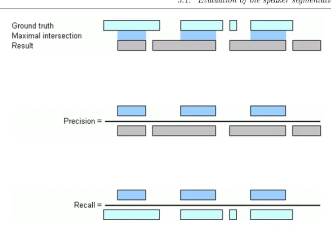
3.1 The Argos precision and recall measures in respect to the ground truth segmen-tation and the system segmensegmen-tation. . . 49

3.2 Comparison between the precision of BIC, GLR-BIC and Iterative system seg-mentation methods on the 20 files of ESTER-2 development set. . . 51

3.3 Comparison between the recall of BIC, GLR-BIC and Iterative system segmen-tation methods on the 20 files of ESTER-2 development set. . . 52

(17)

List of Figures

4.1 Examples of rectangle features: (A) and (B) show two-rectangle feature, (C) shows

a three-rectangle feature, (D) shows a four-rectangle feature [VJ01]. . . 74

4.2 A face image and its corresponding sift features. . . 82

5.1 General architecture of the people indexing system. . . 86

5.2 Multi-face frontal detection on a still image. . . 88

5.3 Extraction of clothing using frontal faces. . . 89

5.4 Extracting and modeling the color of the skin within the face. . . 90

5.5 Examples of skin color extraction within the face: For each face image, the corresponding extracted skin part image appears below it. . . 91

5.6 The backward-forward tracking scheme. . . 92

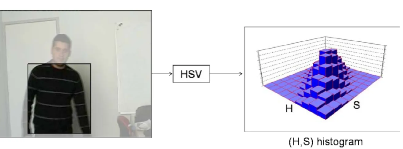
5.7 2D histogram for the H and S components computed on the clothing zone. . . 94

5.8 Choice of the key-face. . . 96

5.9 Example of good matches under some variation in lighting, orientation and scale. 97 5.10 Example of bad matches. . . 97

5.11 Example of 13 faces of the same person that were correctly matched using ANMPD distance: we can notice different facial expressions, lightning conditions, glasses and occlusions. This example is taken from the AR database [MB98]. . . 99

5.12 Two people with two different costume box: the noise is due to the background and to the foreground objects like hands and characters. . . 100

5.13 Extraction of the dominant color. . . 101

5.14 Examples of dominant color areas extracted. . . 102

5.15 First-level hierarchical clustering. . . 105

6.1 Comparison between the four features and the proposed clustering method. . . . 112

6.2 Comparison between applying the Histogram comparison directly on the costume box and applying it on the dominant color area. . . 113

6.3 Example 1 of cluster delivered at the end of the clustering process of “arret sur image” TV debates. . . 113

6.4 Example 1 of cluster delivered at the end of the clustering process of “arret sur image” TV debates. . . 114

6.5 Example of a cluster delivered at the end of the clustering process on the ABC news. . . 116 xiv

(18)

6.6 Example of a cluster delivered at the end of the clustering process on the CNN

news. . . 117

6.7 Example 1 of a cluster delivered at the end of the clustering process on France 2 news. . . 117

6.8 Example 2 of a cluster delivered at the end of the clustering process on the France 2 news. . . 118

6.9 Example of a cluster delivered at the end of the clustering process on the LBC news. . . 118

6.10 Example of a cluster delivered at the end of the clustering process on the CCTV news. . . 119

6.11 Example 1 on “le Grand Journal”. . . 120

6.12 Example 2 on “Le Grand Journal”. . . 121

6.16 Example on “C’est dans l’air”. . . 123

6.17 Example of the movie “Amelie”. . . 123

6.18 Example 1 of the movie “Asterix et Obelix”. . . 124

6.19 Example 2 of the movie “Asterix et Obelix”. . . 124

6.20 Example 1 of the movie “Virgins suicide”. . . 125

6.21 Example 2 of the movie “Virgins suicide”. . . 125

7.1 Different types of fusion defined by Dasarthy [Das94]. . . 137

8.1 Number of frames for each character appearance, on a TV talk show. . . 148

8.2 A list containing the output of the association process. . . 151

8.3 Talking person appearing with the audience in a TV debate. . . 152

8.4 Three faces detected with their corresponding weights. . . 153

8.5 Two faces with different sizes but similar weights. . . 154

8.6 Mouth localization using geometrical constraint. . . 155

8.7 Lips activity curve. . . 156

8.8 Architecture of the audio-visual people indexing system. . . 160

(19)

List of Figures

9.1 Example 1 of the movie “Les Choristes”. . . 168

9.2 Example 2 of the movie “Les Choristes”. . . 168

A.1 Variation of Feature F1 for 3 consecutive programs. . . 182

A.2 Distribution of Feature F1 for 3 consecutive programs. . . 183

A.3 Variation of Feature F3 for the same 3 consecutive programs. . . 184

A.4 Distribution of Feature F3 for the same 3 consecutive programs. . . 185

C.1 The output file in the XML format. . . 190

(20)

General Introduction

You’re resting on your sofa, watching your favorite series on your HQ television. At the same time, you’re reading your electronic version of the New York Times on your laptop, downloading a new song on your smart phone. Suddenly, you remember one of the “Charlie Chaplin” black and white movies. You open the Youtube web page, type few words, and instantly get it and start viewing it... While watching, memories take you back to the past, to the first time you watched color TV, the first time you used mobile phone, the first time you recorded a CD... What? like a zillion years ago?... That is how fast are the advances in data capturing, storage, indexing, and communication technologies!

1 Context

Since many decades, the multimedia technologies have facilitated the way delivering data to customers, and connecting with banks of audio, image, text and video information. Actually, billions of video files are viewed1 and thousands of them are created every day. However, there are still limited tools to index, characterize, organize and manage these data. Thus, there are still limited applications that allow users interacting with them. Manually generating a description of audiovisual content of data is not only very expensive, but sometimes, time consuming, subjective and inaccurate.

It was obvious that many laboratories and scientist started giving the domain of multimedia indexing a special attention, and joining the efforts to propose new algorithms that enable fast and accurate access to the information the consumer is asking for. Since an audiovisual document is basically multimodal, and since the content of those media are generally correlated, recent research activities are focusing on finding ways to combine useful information coming from audio, video, image and text to enhance the content based multimedia indexing.

1

(21)

General Introduction

The SAMOVA2team of the IRIT3laboratory was born in 2002 with the goal of exploiting the audio and video media, and to study the correlation between them. In the audio domain, we may include works carried on speech activity detection [PRAO03], language recognition [RFPAO05], singing detection and music characterization [LAOP09], etc. In the video domain, we may include works carried on human shape analysis [FJ06], person labeling using clothing [Jaf05], etc. In audiovisual domain, we may include works carried on dynamic organization of database using a user-defined similarity [PPJC08], similarity measures between audiovisual documents [HJC06], etc4. During this process, it has been found that person characterization was not paid enough attention except the orphan work on clothing.

In almost every audiovisual document, persons appear, interact and talk. Thus detecting, tracking, classifying and identifying them have very significant impacts on the knowledge of that document, and enable a huge amount of applications.

The work of this thesis is essentially focused on video indexing based on audiovisual charac-terization of persons. To be as generic and training-free as possible, we decide solving this task with an unsupervised manner.

2 Characterization of persons

The characterization of persons within an audiovisual document is one of the challenging prob-lems in current research activities. Many of them have addressed this problem with only one modality.

From the audio point of view, the characterization of persons is generally known as speaker diarization: it aims to segment the audio stream into turns of speakers and then cluster all turns that belong to the same speaker. In other meanings, its goal is to answer the questions “who talk? and when?”.

From the video point of view, the characterization of persons is generally known as people detection, tracking and recognition. In other words, it aims to answer the questions “who appear? and when?”.

2_{Structuration, Analyse et Modelisation des documents Video et Audio.} 3

Institut de Recherche en Informatique de Toulouse: http://www.irit.fr

4

http://www.irit.fr/recherches/SAMOVA/

(22)

3. Our Contribution

A few other research activities have addressed the problem of persons characterization from a multimodal point of view. However their applications are generally limited and constrained. Thus, we may define this task by trying to answer the following questions:

- “Who talk and appear? and when?”

- “Who talk without appearing? and when?” - “Who appear without talking? and when?”

3 Our Contribution

Our main contribution in this Ph.D, financed by the French Ministry of Education, can be divided into three parts:

• Propose an efficient audio indexing system that aims to split the audio channel into homogeneous segments, discard the non-speech segments, and group the segments into clusters, that each corresponds ideally to one speaker. This system must process without a priori knowledge (unsupervised learning) and must be suitable to any kind of data: TV/radio broadcast news, TV/radio debates, movies, etc.

• Propose an efficient video indexing system that aims to split the video channel into shots, detect and track people in every shot, and group all faces into clusters, that each corresponds ideally to one person. This video system must process without a priori knowledge and may be suitable to any kind of data.

• Propose an efficient audiovisual indexing system that aims to combine audio and video indexing systems in order to deliver an audiovisual characterization of each person talking and/or appearing in the audiovisual document, and a robustified audio indexing output (respectively video indexing output) using the help of video (respectively the aid of audio).

4 Organization of this report

This report is composed of three main parts:

1. Part I considers the audio channel: state-of-the-art methods for speaker diarization are reviewed in chapter 1, our proposed audio indexing system is described in chapter 2, and the experiments and the results are detailed in chapter 3.

(23)

General Introduction

2. Part II considers the video channel: existing methods for people detection, tracking and recognition are reviewed in chapter 4, our proposed face-and-clothing based people index-ing system is presented in chapter 5, and the experiments and the results are described in chapter 6.

3. Part III considers the fusion between audio and video descriptors: existing works on audiovisual fusion are detailed in chapter 7, our proposed audiovisual association system is described in chapter 8, and the experiments and the results are shown in chapter 9.

(24)

Part I

(25)

(26)

Introduction

Most of works in audio indexing are leading to annotate an input audio signal with information that attributes temporal regions of signal to their specific sources/classes and then to give a special ID to each class. These IDs may identify particular speakers, music, background noise or other signal sources like animal voices, applause, etc. Even though we are only interested in the issue of speaker indexing, it is very important to have a good processing way to get rid of the non speech segments.

The audio speaker indexing aims to detect speaker identity changes in a multi-speaker audio recording and classifies each detected segment according to the identity of the speaker. It is sometimes confused with speaker diarization that consists in answering the question “Who spoke when?”. In another meaning, its purpose is to locate each speaker turn and to assign it to the appropriate speaker cluster. The output of the corresponding system is a set of segments with a unique ID assigned to each person. Another definition of speaker diarization is speaker segmentation and clustering. On one hand, the speaker segmentation aims to detect speaker changes in an audio recording. On the second hand, the speaker clustering aims to group segments corresponding to the same speaker into homogeneous clusters.

The general architecture of the speaker indexing system is illustrated in Fig.1.

Domains that receive special research attention are telephone speech, broadcast news (radio, TV) and meetings (lectures, conferences and debates). The corresponding speaker diarization systems have been evaluated by organizations like NIST (National Institute for Standards and Technology) and AFCP (Association Francophone de la Communication Parl´ee).

Hypotheses

In this work, many hypotheses were taken in order to make the problem of speaker diarization the most general and the most useful.

(27)

Introduction

Figure 1: The general architecture of a speaker indexing system.

• Unknown number of speakers. Unlike telephone conversations where almost two people talk, a more realistic case considers that the number of speakers is unknown and one of the final goals is to determine this number.

• No a priori knowledge about speakers and language. We consider that the identity of the speakers in the documents is unknown and that there are no trained models for each 8

(28)

speaker and each language. However, a knowledge about the background is allowed i.e. a universal model separating “studio clean” recording from “outdoor noisy” recording can be trained.

• Not only speech. Recording speech data contain generally in addition to speech, music and other non-speech sources. Thus, the realistic choice is to build a system that first detects the speech and non speech regions in order to enable processing on the speech regions on later stages.

• People may talk simultaneously. In many existing systems, this hypothesis was ne-glected or at least not paid a special attention. Effectively, this is not very important if the data processed are broadcast news: in this case, the speech is even prepared previously and then read, or at least “speakers are polite”. But in some meeting or translation conditions, it is obvious that we should take care of this assumption.

Applications

Audio speaker indexing is very useful in many types of applications because it provides extra information according to the speakers. By adding this knowledge to speech transcripts, it becomes easier for humans to localize relevant information and for speech translation systems to process it. Some of those applications may be:

• Indexing audio recording databases. Effectively, this is its first goal because it may be used as a preliminary step in every task of Information Retrieval. Typical automatic uses of such system output might be speech summarization and translation. Coupled with the speaker identification process, it allows, for example, retrieving all speeches of a certain political leader. It may be useful to know the speech duration of each candidate during a presidential campaign. Also, it may be used to retrieve the speech of a journalist in order to identify the topics addressed in a broadcast news recording.

• Automatic Speech Recognition. Speaker segmentation algorithms are used to split the audio recording into small homogeneous segments. Speaker clustering algorithms are also used to cluster the input data into speakers towards model adaptation that is successfully used to improve ASR systems performance.

(29)

Introduction

• Speaker tracking, speaker recognition. Speaker diarization can be used as a pre-processing low-cost module for speaker-based algorithms by splitting the whole data into individual speakers. Thus, the decision is more reliable because it is taken on relatively long segments and huge clusters instead of only some tens of milliseconds.

This part is organized as follows: Chapter 1 presents the state-of-the-art works on speaker diarization. In chapter 2, we detail our proposed methods for speaker segmentation and speaker clustering. Chapter 3 describes the experiments and the results.

(30)

Chapter 1 State-of-the-art of Speaker

Diarization

Contents

1.1 Acoustic Features . . . 12

1.2 Audio event segmentation . . . 13

1.3 Audio speaker segmentation . . . 14

1.3.1 Segmentation by silence detection . . . 15

1.3.2 Segmentation by speaker change detection . . . 15

1.4 Audio speaker clustering . . . 21

1.4.1 BIC based approaches . . . 23

1.4.2 Eigen Vector Space Model approach . . . 23

1.4.3 Cross Likelihood Ratio clustering . . . 24

1.4.4 Hidden Markov Model approach . . . 25

1.4.5 Other clustering techniques . . . 26

1.5 Examples of state-of-the-art speaker diarization systems . . . . 26

1.5.1 The LIMSI speaker diarization system . . . 26

1.5.2 The IBM speaker diarization system . . . 27

1.5.3 The LIA speaker diarization system . . . 28

1.6 Databases . . . 30

1.6.1 ESTER-1 Corpus . . . 30

(31)

Chapter 1. State-of-the-art of Speaker Diarization

1.6.3 EPAC-ESTER Corpus . . . 30

In this chapter, the main existing techniques for speaker diarization are reviewed. First, the acoustic features that have been found useful for speaker diarization are listed in section 1.1. In section 1.2, a brief look on the audio event segmentation is presented. Then, the different approaches used for speaker segmentation and speaker clustering are respectively described in sections 1.3 and 1.4. Some of the famous existing systems are presented in section 1.5. The databases used in our work are described in section 1.6.

1.1 Acoustic Features

Acoustic features extracted from the audio recording provide information on the speakers during their conversation. This information allow the system to separate them correctly.

As for many speaker-based processing techniques, the cepstral features are the mostly used in speaker diarization systems. These parametrization features are: the Mel Frequency Cepstrum Coefficients (MFCC), the Linear Frequency Cepstrum Coefficients (LFCC), the Linear Predictive Coding (LPC), etc.

Moreover, in the area of audio event segmentation (speech, music, noise and silence), features like the energy or the 4 Hertz modulation energy were shown to be useful for speech detection. Other features like the number and the duration of the stationary segments obtained from a forward/backward segmentation [AO88] are used for example for music detection.

In addition, some frequential information like the pitch frequency and the harmonical fre-quencies are used to separate for example males from females in the speech part.

In the following subsections, the acoustic features used in our work are detailed:

• Mel Frequency Cepstrum Coefficients. The ceptral information of an audio signal allows to separate the glottal excitation and the resonance of the vocal tract. By filtering the signal, only the contribution of the vocal tract is kept. MFCCs were introduced in [Mer76]. They are generally derived as seen in Fig.1.1. After windowing the signal using Hamming approximation, the Fourier transform is computed on every window, then the powers of the spectrum are mapped onto the MEL scale using triangular overlapping windows. After that, the logs of the powers of each of the MEL frequencies are taken. Finally the inverse of the fast Fourier transform of the list of Mel log powers are computed. 12

(32)

1.2. Audio event segmentation

Thus, the MFCCs are the amplitudes of the resulting spectrum. Practically, a MFCC vector is extracted every 10 milliseconds on a shifted Hamming window of 20 milliseconds.

Figure 1.1: Creating the MFCC features of a signal x.

• 4 hertz modulation energy. Unlike the music signal, the speech signal has an energy modulation peak around the 4 Hz syllabic rate (4 syllables per second). This property was used in [PRAO03] to separate speech from music, but also can be used to distinguish clean speech from noisy speech, or mono-speaker speech from interaction zones where two or more people talk simultaneously. Typically, a value of the 4 Hz modulation energy is computed every 16 milliseconds.

• Pitch frequency. This feature characterizes the gender of the speaker. The pitch fre-quency of the voice is generally around 150 Hertz for a man. In opposite, it is around 250 hertz for a woman and around 350 hertz for children. This property can be used to help the clustering process. Moreover, algorithms used to estimate this pitch can help the speech detection and music detection because unlike instrumental voices, a normal human voice cannot be less than 60 Hz and higher than 400 Hz. In this work, we used the pitch estimators of The Snack Sound Toolkit5.

• Number and duration of segments provided by the forward/backward segmentation method [AO88]. This segmentation method estimates the boundaries of every phonetic unit present in the acoustic signal. Unlike speech signal, music signal is characterized by a relative lower number of those units and a higher value of their duration.

1.2 Audio event segmentation

Known as “Segmentation en Ev´enements Sonores”(SES) by the french community, the output of such a segmentation is a list containing the starting and the ending times of all the audio

5

(33)

events that occur in the audio recording. Those events are: speech, speech, music, non-music and (speech + non-music). Typically, a SES system is used as a preprocessing step for the speaker diarization system and, to the best of our knowledge, all existing methods build those two systems completely separatly. That is why the results of the second system are directly related to the output of the first one: if the turns of speaker X were not detected as speech by the SES system, X will be missed and there is no possibility to find it again. As seen in section 2.3, we describe a framework to handle this weakness by proposing an iterative system that enables both audio event segmentation and speaker diarization.

The task of audio event segmentation can be divided into two main issues:

On one hand, algorithms used for speech activity detection are often based on Gaussian Mixtures Models (GMMs) for both Speech and Non-Speech components [GL94] using the MFCC vectors. Those models need learning and depend on the training data. However, unsupervised methods use robust features like the 4Hz modulation energy described in the previous section that practically is affected by the database variation.

On the other hand, algorithms used for music detection are also based on both supervised methods using GMMs on MFCCs and unsupervised methods using the number and the duration of segments as explained previously.

The fusion of supervised and unsupervised methods was developed at the IRIT Laboratory and gave results among the best on ESTER-1 database (cf. section 1.6.1 [GGM+_{05]. For more}

details about those methods, please refer to [PRAO03]. Recently, methods bases on Support Vector Machine (SVM) are shown to provide a slightly better performance [TMN07].

1.3 Audio speaker segmentation

Speaker segmentation consists in segmenting the audio recording into homogeneous segments. Each segment must be as long as possible and must contain the speech of one speaker. This segmentation is closely related to acoustic change detection as it will be pointed out later on (cf. section 2.3).

Two main categories of speaker segmentation can be found in the literature: the segmentation by silence detection and the segmentation by speaker change detection. Those two techniques are explained in the following subsections.

(34)

1.3. Audio speaker segmentation

1.3.1 Segmentation by silence detection

It is the intuitive and trivial solution to separate turns of speaker in the audio recording. It assumes that changes between speakers happen through a silence segment. A silence is characterized by a low energy level. For some types of data like telephone conversations where the noise is strongly present, this hypothesis is not realistic. Most existing methods for silence detection use:

- the mean power of the signal. This is the simplest way to detect silence [NA99]. This method encounters two main problems. First, the choice of the threshold used to isolate silence is not very stable because it depends on the processed data. Then, the boundaries are not well detected because the mean average of the power is computed every 0.5 or 1 second.

- the histogram of the energy. This method [MC98] splits the audio recording into segments of 15 seconds. The histogram of each segment is approximated by a Gaussian distribution. If the segment is shown to be homogeneous in terms of the probability density function, it is indexed as silence or non-silence. If it is not the case, the segment is splitted by using the k-means algorithms that computes the average mean and the standard deviation of both silence and non-silence parts.

- the variability of the energy. This method [GSR91] consists in computing the vari-ability of the energy for a signal portion. If the varivari-ability is low, then this portion is considered as silence. If this variability is high, it is considered as speech.

- the zero-crossing rate. The silence, besides being characterized by a low-level energy, has a high zero-crossing rate [TP99]. This rate represents the number of times the signal has zero amplitude by temporal unit.

All approaches for speaker segmentation by silence detection need a threshold that depends on the audio document. Furthermore, there is no efficient method to determine optimally this threshold.

1.3.2 Segmentation by speaker change detection

The speaker change detection (SCD) is the most common method used for speaker segmentation. It aims to detect boundaries for each speaker turn within the audio recording even if there is

(35)

no silence between two consecutive speakers. That explains the numerous existing methods for SCD and why speaker segmentation has sometimes been referred to as SCD.

Technically, two main types of SCD systems can be found in the bibliography. The first kind are systems that perform a single processing pass of the audio recording. The second kind are systems that perform two-pass algorithms: in the first pass, many points of change are suggested with a high false alarm rate. Then, in the second pass, those points are re-evaluated and some are discarded in order to converge into an optimum speaker segmentation output.

In the following sections are presented some existing methods that were successfully used for SCD. Those methods were applied for either a single processing pass or multiple processing passes. Moreover, they can be classified into three categories: metric-based approaches like the symmetric Kullbach-Leibler (KL2) distance, model-based approaches like the Generalized Likelihood Ratio (GLR) and the Bayesian Information Criterion (BIC), and mixed approaches like the Hotelling T2-Statistics and BIC.

1.3.2.1 Symmetric Kullbach-Leibler divergence

The Kullbach-Leibler [KL51] measures the difference between the probability distributions of two continuous random variables. It is given by:

D(p1, p2) = Z +∞ −∞ p1(x)ln( p1(x) p2(x) )dx (1.1)

Because this expression is not symmetric in respect to the two variables, the symmetric KL (KL2) is proposed:

∆ = D(p1, p2) + D(p2, p1)

2 (1.2)

When the distributions are Gaussian N1(µ1,σ1) and N2(µ2,σ2), it becomes:

∆ = 1 2[ σ₁2 σ₂2 + σ₂2 σ₁2 + (µ1− µ2) 2₍ 1 σ2₁ + 1 σ₂2)] (1.3)

where µi represent the mean average and σi the covariance of a Gaussian distribution Ni.

In [SJRS97], the KL2 is used as follows: for every point of the audio recording, the two adjacent windows from both sides are considered. The duration of each window is fixed to 2 seconds. The mean and the covariance are estimated on each window. Thus, the KL2 distance can be easily computed. This process is repeated for every point so a distance curve is drawn and the local maxima are detected. Those local maxima correspond ideally to points of speaker changes.

(36)

1.3.2.2 Generalized Likelihood Ratio

For genericity reasons that will be addressed later in this chapter, we will describe this method using an unknown signal that may be an acoustic signal, a video signal or an audiovisual signal. Let X = x1, . . . , xNx be the sequence of observation vectors of dimension d to be modeled and

M the estimated parametrical model and L(X, M ) the likelihood function. The GLR introduced by Gish et al. [GSR91] considers the two following Hypotheses:

- H0: This hypothesis assumes that the sequence X corresponds to only one homogeneous

segment (in the case of audio signal, it corresponds to only one audio source). Thus, the sequence is modeled by only one multi-Gaussian distribution.

(x1, . . . , xNx) v N (µX, σX) (1.4)

- H1: This hypothesis assumes that the sequence X corresponds to two different homogeneous

segments X1 = x1, . . . , xi and X2 = xi+1, . . . , xNx (in the case of audio signal, it

corre-sponds to two different audio sources or more particularly to two different speakers). Thus, the sequence is modelled by two multi-Gaussian distributions.

(x1, . . . , xi) v N (µX1, σX1) (1.5)

and

(xi+1, . . . , xN) v N (µX2, σX2) (1.6)

The generalized likelihood ratio between the hypothesis H0 and the hypothesis H1 is given by:

GLR = P (H0) P (H1)

(1.7) In terms of likelihood, this expression becomes:

GLR = L(X, M )

L(X1, M1)L(X2, M2)

(1.8) If this ratio is lower than a certain threshold T hr, we can say that H1 is more probable, so

a point of change in the signal is detected. By passing through the log:

(37)

and by considering that the models are Gaussian, we obtain:

R(i) = NX 2 log |ΣX| − NX1 2 log |ΣX1| − NX2 2 log |ΣX2| (1.10)

where ΣX, ΣX1 and ΣX2 are the covariance matrices of X, X1 and X2 and NX, NX1 and

NX2, are respectively the number of the acoustic vectors of X, X1 and X2.

Thus, the estimated value of the point of change by maximum likelihood is given by:

bi = arg max

i R(i) (1.11)

If bi is higher than the threshold T = −logT hr, a point of speaker change is detected. The major disadvantage resides in the presence of the threshold T that depends on the data. That is why, Rissanen [Ris89] introduced the Bayesian Information Criterion (BIC).

1.3.2.3 Bayesian Information Criterion For a given model M, the BIC is expressed by:

BIC(M ) = log L(X, M ) −λ

2n log NX (1.12)

where n denotes the number of the observation vectors of the model. The first term reflects the adjustment of the model to the data, and the second term corresponds to the complexity of the data. λ is a penalty coefficient theoretically equal to 1. [Ris89].

The hypotheses test of Equ.1.7 can be viewed as the comparison between two models: a model of data with two Gaussian distributions (H1) and a model of data with only one Gaussian

distribution (H0). The subtraction of BIC expressions related to those two models is:

∆BIC(i) = R(i) − λP (1.13)

where the log-likelihood ratio R(i) is already defined in Equ.1.10, and the complexity term P is given by:

P = 1 2(d +

1

2d(d + 1)) log NX (1.14)

d being the dimension of the feature vectors.

The BIC can be also viewed as the thresholding of the log-likelihood distance with an automatic threshold equal to λP .

(38)

Thus if ∆BIC(i) is positif, the hypothesis H1 is privileged (two different speakers). There

is a change if:

{max

i ∆BIC(i) ≥ 0} (1.15)

The estimated value of the point of change can also be expressed by:

bi = arg max

i ∆BIC(i) (1.16)

Chen et al [CG98] used this criterion to segment the data of the DARPA evaluation campaign. They said that the BIC procedure has the advantage of not using a threshold, because at that time, the existing methods used thresholds and the retrieving of the optimal thresholds was so complicated. But they forgot the penalty coefficient λ that is practically not necessarily equal to 1.

Many multi-points detection algorithms based on BIC were then developed. In [TG99], Tritschler used a shifted variable size window to detect the points of speaker change in a broadcast news audio recording. Then, the authors of [Cet00], [DW00], [SFA01] and [CV03] proposed improvements in order to obtain either more accurate detection or faster computational time. Fig.1.2 illustrates the segmentation process used in [SFA01] and [CV03]: it shows that there are 8 parameters that should be carefully tuned and that depend from the processed data. This weakness motivated us to propose a parameters-free method as seen later in section 2.1.

1.3.2.4 Hotteling T2_{-Statistics with BIC}

It can be easily shown that the segmentation algorithms based only on BIC have a quadratic complexity. Even if we can improve the time machine by sampling the audio signal, the com-putational cost stays relatively high because we should compute two full covariance matrices in each shifted variable size window.

Moreover, when estimating the mean and the covariance, the segmentation error is relatively high if the acoustic events have short durations. That is why, Zhou et al. [ZH05] used an approach for SCD using the T2_{−statistics and BIC.}

(39)

Figure 1.2: The multiple change detection algorithm used by [SFA01] and [CV03].

The T2−statistics expression is given by:

T2 = i(NX − i) NX

(µX1 + µX2)

0_Σ−1_(µ

X1 − µX2) (1.17)

where i corresponds to the point of change, Σ the common covariance matrix, µX1 and µX2 the

estimated mean average of the Gaussian models of the two sub-windows separated by the point i. For more details about the combination between the T2−statistics and the BIC, please refer to [ZH05].

In addition to the above techniques, there are few works that use the dynamic program-ming to find the speaker change points [VCR03], the Maximum Likelihood (ML) coupled with BIC [ZN05], or genetic algorithm [SSGALMBC06] where the number of segments is estimated via the Walsh basis function and the location of change points is found using a multi-population genetic procedure.

(40)

1.4. Audio speaker clustering

1.4 Audio speaker clustering

At the end of the speaker segmentation process, segments that contain the speech of only one speaker are provided. The next step aims to agglutinate together all segments that belong to the same speaker. This step of clustering can be used in many applications: for example, Automatic Speech Recognition (ASR) systems use homogeneous clusters to adapt the acoustic models using MAP (Maximum A Posteriori ) to the speaker and so increase recognition performance.

This blind speaker clustering with no a priori information about the number of people and their identities, can be viewed as an unsupervised classification problem. In general, unsupervised classification methods use a hierarchical clustering.

Hierarchical clustering

The goal of the hierarchical clustering is to gather iteratively a set of elements. There are two approaches illustrated in Fig.1.3: the bottom-up clustering and the top-down clustering. The first one considers at the beginning every element as a cluster and merge after each iteration the two most similar clusters in terms of a merging criterion. This process is repeated until a defined stopping criterion is verified. Contrarily, the top-down clustering considers at the beginning the whole set of elements as only one cluster and then, after each iteration, splits the cluster in terms of a splitting criterion. This process is repeated until the stopping criterion is verified.

(41)

The Bottom-up clustering known also as agglomerative clustering is by far the mostly used in the literature because it uses the output speaker segmentation techniques to define a clustering starting point.

In the design of such systems for speaker clustering, the merging/splitting criterion C corresponds to the distance/similarity between clusters. And sometimes, instead of defining an individual value pair, a distance/similarity matrix is described, which is created with the distance/similarity from any possible pair.

More precisely, the criterion C between two clusters of elements G1 and G2 can be expressed

in different possibilities:

• single linkage: also known as minimum pair, the clustering criterion C is defined as the minimum criterion separating two elements, each belonging to one cluster.

C(G1, G2) = min i∈G1,j∈G2

C(i, j) (1.18)

• complete linkage: also known as maximum pair, the clustering criterion C is defined as the maximum criterion separating two elements, each belonging to one cluster.

C(G1, G2) = max i∈G1,j∈G2

C(i, j) (1.19)

• average linkage: also known as average pair, the clustering criterion C is defined as the mean average criterion of all pairs of elements, each belonging to one cluster. N1 and N2

denote the number of elements respectively of G1 and G2 in the following formula.

C(G1, G2) =

Σi∈G1,j∈G2C(i, j)

N1N2

(1.20)

• full linkage: unlike the above linkage methods, this method considers a class of elements as only one element ( in our case, a cluster of segments is considered as only one segment obtained by the concatenation of all the segments in the cluster). The characteristics of each class are re-computed at the end of every iteration. That involves a huge computa-tional cost of the clustering process unlike previous methods.

The following subsections review the main systems existing in the literature for speaker clus-tering. Even though some of them may be suitable for online configuration where no information on the complete recording is available, the systems listed below were initially developed for an offline configuration where they have access to the whole recording file before processing it. 22

(42)

1.4.1 BIC based approaches

The Bayesian Information Criterion that was well explained for speaker segmentation is by far the most commonly used distance and merging criterion for speaker clustering. It was initially proposed for clustering by Chen et al. in [CG98]. The pair-wise distance matrix is computed for each iteration and the pair with the lowest ∆BIC value is merged. The process finishes when all pairs have a ∆BIC > 0. Considering two clusters G1 and G2, each of those clusters is

modeled by a multi-Gaussian distribution. The ∆BIC distance is given by:

∆BIC(G1, G2) = (n1+n2) log |Σ|−n1log |Σ1|−n2log |Σ2|−

λ 2(d+

d(d + 1)

2 )log(n1+n2) (1.21) where n1, n2 are the sizes of G1 and G2. Σ1, Σ2 and Σ are respectively the covariance matrices

of G1, G2 and G1S G2. d is the dimension of the feature vectors.

1.4.2 Eigen Vector Space Model approach

This method proposed by Tsai [TCCW05] uses the vector space model, which was originally developed in document-retrieval research, to characterize each utterance as a tf-idf -based vector of acoustic terms, thereby deriving a reliable measurement of similarity between utterances. Fig.1.4 describes the EVSM algorithm.

Figure 1.4: The EVSM-based algorithm.

To begin, a “universal GMM” is created using all the segments to be clustered. The training method is based on the k-means clustering initialization followed by Expectation-Maximization (EM). An adaptation of universal GMM is then performed for each of the utterances using max-imum a posteriori (MAP) estimation. This gives N utterance-dependent GMMs λ1, λ2, ..., λN.

(43)

The use of such a model adaptation instead of a direct EM-based training of GMM has two-fold advantages. One is to produce a more reliable estimate of the GMM parameters for short utterances than it can be done with direct EM-based training. The other is to force the mixtures of all the utterance-dependent GMMs to be of the same order.

Next, all the mean vectors of each utterance-dependent GMM are concatenated in the order of mixture index to form a super-vector, with dimension of D. Then, Principal Component Analysis (PCA) is applied to the set of N super-vectors, V1, V2, ..., VN, obtained from N

utterance-dependent GMMs. This yields D eigenvectors, e1, e2, ..., eD, ordered by the magnitude of their

contribution to the between-utterance covariance matrix:

B = 1 N N X i=1 (Vi− V )(Vi− V )0 (1.22)

where V is the mean vector of all Vi for 1 < i < N . The D eigenvectors constitute an

eigenspace, and each of the supervectors can be represented by a point on the eigenspace:

Vi= V + D

X

d=1

φi,ded (1.23)

where φi,d, 1 ≤ d ≤ D, is the coordinate of Vi on the eigenspace. Then, the authors

use the cosine formula for each pair of vectors in order to quantify the similarity between the corresponding pair of segments/clusters.

Si,j(Vi, Vj) =

Wi· Wj

kWik kWjk

(1.24)

where Wi and Wj are the vector Vi and Vj obtained after the reduction of the dimension.

1.4.3 Cross Likelihood Ratio clustering

The Cross Likelihood Ratio (CLR) clustering was used as a final step of a posteriori clustering in many speaker diarization systems as in [RSC+98] and [ZBMG05]. After a first step of clustering (using for example the BIC clustering), the background environment contribution in the cluster models must be reduced and normalized in order to allow additional clustering for speakers whose environmental conditions change during their speech. Moreover, the size of the clusters is good enough to allow building a more complex and robust speaker model, such as Gaussian Mixture Model (GMM), for each cluster. Thus, a universal background model (UBM) should 24

(44)

be learned and then adapted for each cluster, providing the initial speaker model. After each iteration, the clusters that maximize the Cross Likelihood Ratio (CLR) are merged:

CLR(G1, G2) = L(G1/M2) L(G1/U BM ) × L(G2/M1) L(G2/U BM ) (1.25)

Where M1, M2are the models associated to the clusters G1and G2, and UBM is the universal

background model and L(.) is the likelihood. When the CLR(G1, G2) is greater than an a priori

threshold thr, the clustering step stops to merge.

The UBM results from the fusion of four models which are gender (male/female) and band-width (narrow/wide bands) dependent models with 128 diagonal covariance components. Then, the cluster model is derived from the UBM by MAP adaptation (means only).

Although the UBM model could be learned once, the evaluation of CLR clustering done in [BZMG06] shows that the threshold may depend on the corpus.

1.4.4 Hidden Markov Model approach

The Hidden Markov Model (HMM) was also used for speaker clustering. Every state in the model represents a cluster and the transitions between states characterize the changes between speakers.

In [ALM02], the clustering is composed of several sub-states to impose the minimum duration constraints considering that the HMM is ergodic in nature. The probability density function (PDF) of each state is represented by a GMM. The process starts by over-clustering the data (larger number of clusters than the expected number of speakers). The parameters of the HMM are then trained using the EM algorithm. The merging between two clusters is done using log likelihood ratio (LLR) distance.

In [MBI01], the clustering does not belong to the hierarchical category as all the methods described above. The speaker diarization is done with only one path unlike most of the existing systems that generally separate the segmentation step from the clustering step. The HMM is generated using an iterative process, which detects and adds a new state (i.e. a new speaker) at each iteration. The speaker detection process is composed of four steps:

(45)

2. Adding a new speaker: a new speaker model is trained using 3 seconds of the recording that maximizes the sum of likelihood ratios of model S0. A new state S1 related to that new model is added to the HMM configuration.

3. Adaptation speaker model: the models are adapted after each iteration where new state are created.

4. Assessing the stopping criterion: This criterion is based on the comparison of the proba-bility along the Viterbi path between two iterations of the process.

1.4.5 Other clustering techniques

Unlike the systems described above, there are some clustering methods that define metrics to determine the optimum number of clusters and then to find the optimum clustering given that number.

In [TW07], the optimum amount of speakers is computed using BIC and the optimum clus-tering that optimizes the overall model likelihood is obtained by a genetic algorithm. In [Roy97], a speaker indexing algorithm is proposed to dynamically generate and train a neural network to model each postulated speaker found within a recording. Each neural network is trained to differentiate the vowel spectra of one specific speaker from all other speakers. In [Lap03], self-organizing maps are proposed for speaker clustering using a Vector Quantization (VQ) algorithm for training the code-books representing each of the speakers.

1.5 Examples of state-of-the-art speaker diarization systems

Many systems exist in the literature and were evaluated in international/national competitions. In the following subsections, we choose to review three of those famous systems.

1.5.1 The LIMSI speaker diarization system

The Speaker Diarization (SD) system described here was used by the LIMSI6 in the Rich Transcription (RT) evaluation conducted by NIST in 2007 on meeting and lecture recordings. This system [ZBLG08] is built upon the baseline diarization system designed for broadcast news data and it combines an agglomerative clustering based on BIC with a second clustering using

6

http://www.limsi.fr/

(46)

1.5. Examples of state-of-the-art speaker diarization systems

state-of-the-art speaker identification (SID) techniques. This system is similar to the LIUM7 system that gives the best results in the last ESTER competition.

Speech is extracted from the signal by using a Log-Likelihood Ratio (LLR) based speech activity detector (SAD). The LLR of each frame is computed between the speech and non-speech models with some predefined prior probabilities. To smooth LLR values, two adjacent windows with a same duration are located at the left and right sides of each frame and the average LLR is computed over each window. Thus, a frame is considered as a possible change point when a sign change is found between the left and right average LLR values.

Initial segmentation of the signal is performed by a local divergence measure between two adjacent sliding windows. A Viterbi re-segmentation is applied to adjust segments boundaries. A first agglomerative clustering is processed using BIC. Then, speaker recognition methods are used: feature warping normalization is performed on each segment in order to map the cepstral feature distribution to a normal distribution and reduce the non-stationary effects of the acoustic environment. The GMM of each remaining cluster is obtained by maximum a posteriori (MAP) adaptation of the means of a universal background model (UBM) composed of 128 diagonal Gaussians. The second stage of agglomerative clustering is carried out on the segments according to the cross log-likelihood ratio.

1.5.2 The IBM speaker diarization system

The SD system described here was used by the IBM8 in the RT07. In summary, the sys-tem [HMVP08] has the 3 following characteristics:

• the use of an SAD algorithm based on a speech/non-speech HMM decoder, set to an optimal operating point for “missed speech / false alarm speech” on development data.

• the use of word information generated from Speech to Text (STT) decoding by means of a speaker-independent acoustic model. Such information is useful for two reasons: it filters out short silence, background noise, and vocal noise that do not discriminate speakers and it provides more accurate speech segments to the speaker clustering step.

• the use of the GMM-based speaker models that are built from the SAD segmentation. The labels of each frame are refined using these GMM models, followed by smoothing

7

http://www-lium.univ-lemans.fr/

8

(47)

the labeling decision with its neighbors. This method was used to detect change points accurately within the speech segments.

1.5.3 The LIA speaker diarization system

The SD system described here was also used by the LIA9 in the RT07. This system [FE08] is structured of 4 main steps:

1. a speech/non-speech detection using the Linear Frequency Cepstrum Coefficients (LFCC) is based on a two state HMM. Those two states represent speech and non-speech events. Each of those states is initialized with a 32-component GMM model trained using Expectation-Maximization (EM) and Maximum Likelihood (ML) algorithms.

2. a pre-segmentation based on the GLR criterion is used in order to initialize and speed-up the later segmentation and clustering stages.

3. a unique algorithm for both speaker segmentation and clustering is performed using an evolutive hidden Markov model (E-HMM) where each E-HMM state characterizes a single speaker and the transitions represent the speaker turns.

4. a post-normalization and re-segmentation is applied to facilitate the estimation of the mean and variance on speaker-homogeneous segments.

Table 1.1 illustrates the main difference between the three above systems.

Even though the robustness of those system shown by their performance, there are still some points that can be improved:

- preprocessing by removing all non-speech parts using thresholding methods. First, it will be better to split the stream into homogenous zones, and then make the decision on those zones: this decision will be more confident. Second, the use of diarization information (i.e. audio clusters) is helpful to make decision on regions of doubt where the values are on borders (i.e. close to the threshold).

- there is generally reverse connections between the different steps of the system: it will be better to use, for example, not only the segments in order to create the clusters, but also the clusters in order to rectify the segments (by splitting or changing borders).

9

http://www.lia.univ-avignon.fr/

(48)

1.5. Examples of state-of-the-art speaker diarization systems

Table 1.1: Comparison between three state-of-the-art systems.

LIMSI IBM LIA

Acoustic features MFCC + (their 1st and 2nd derivatives) + (1st and 2nd derivatives of the energy) MFCC LFCC Speech Acoustic Detection LLR using 256-components GMM for speech and non-speech HMM decoder using 3-components GMM

for speech and non-speech HMM decoder using 32-components GMM for speech and non-speech Speaker segmentation Gaussian divergence measure + Viterbi re-segmentation using 8-components GMM Speech to Text decoding for segments purification GLR with fixed threshold

Speaker clustering BIC clustering + SID clustering using

128-components GMM Estimation of the initial number of clusters + BIC clustering + refinement using 10-components GMM

E-HMM where every state characterizes a speaker (128-components GMM) Performance at RT’07 on lecture sessions 26% 31% 31%

We will propose in chapter 2 some solutions to overcome those weaknesses without any adaptation on any kind of data (e.g. news, debates and movies).

(49)

1.6 Databases

In order to test our proposed methods and compare them to the state-of-the-art ones, we use three audio recording databases.

1.6.1 ESTER-1 Corpus

ESTER10 which is the French acronym for “Evaluation des Syst`emes de Transcription Enrichie d’´emissions Radiophonique is an evaluation campaign of French broadcast news transcription systems”. The ESTER-1 Corpus (years 2003-2005) includes 100 hours of manually annotated recordings and 1,677 hours of non transcribed data. The manual annotations include the detailed verbatim orthographic transcription, the speaker turns and identities, information about acoustic conditions, and name entities.

The acoustic resources come from six different radio sources, namely: France Inter, France Info, Radio France International (RFI), Radio T´el´evision Marocaine (RTM), France Culture and Radio Classique. For more details on that corpus please refer to [GGM+05].

1.6.2 ESTER-2 Corpus

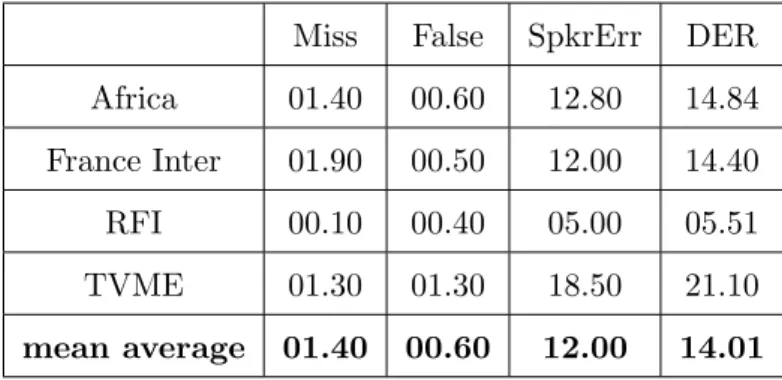
The ESTER-2 Corpus (years 2008-2009) was recorded with the same conditions than the ESTER-1 corpus. It includes 100 hours of manually annotated recordings that come from 5 different radio sources, namely: France Inter, France Info, TVME, Radio Africa 1 and 45 of EPAC-ESTER corpus. Table 1.2 indicates the amount in hours of the annotated data for training, development and test tasks.

1.6.3 EPAC-ESTER Corpus

EPAC11 is the French acronym of “Exploration de masse de documents audio pour l’extraction et le traitement de la parole conversationnelle”. It is a french ANRMDCA project (years 2006 -2009) that gathers four laboratories (IRIT12 , LIA13, LIUM14, LI15) in order to investigate new techniques for automatic speech processing specially in the context of mono-channel meeting

10_{http://www.afcp-parole.org/ester} 11_{http://epac.univ-lemans.fr/} 12_{http://www.irit.fr} 13_{http://www.lia.univ-avignon.fr/} 14 http://www-lium.univ-lemans.fr/ 15 http://www.li.univ-tours.fr/ 30

(50)

1.6. Databases

Table 1.2: Amount of transcribed and non transcribed recordings of ESTER-2.

Source Training Set Development Set Test Set

France Inter 26 h 2 h 3h40 RFI 69 h 40 min 1h10 Africa 1 10 h 2h20 1h TVME - 1 h 1h30 EPAC-ESTER 45 h - -Total 150 h 6 h 7h20

recordings. The EPAC corpus includes 100 hours of manually annotated data. These conver-sational data were selected from the 1,677 hours of the non-transcribed broadcast recording of ESTER-1 Corpus.

(51)

(52)

Chapter 2 Proposed System for speaker

diarization

Contents

2.1 Proposed Generic GLR-BIC segmentation . . . 34

2.1.1 Proposed Method . . . 34

2.1.2 Bidirectional segmentation . . . 36

2.1.3 Penalty coefficient decreasing technique . . . 36

2.1.4 Other applications of the method . . . 38

2.2 Proposed clustering . . . 39

2.2.1 Improved EVSM clustering . . . 39

2.2.2 BIC clustering . . . 40

2.2.3 CLR Post-Clustering . . . 42

2.3 System architecture . . . 44

In this thesis, we investigate new techniques and propose improvements for speaker segmen-tation and speaker clustering. We try to make those techniques the most robust and the most portable for all kind of database (broadcast News, meetings, films, series, TV games).

On one hand, we present a new technique for speaker segmentation. This technique combines the generalized likelihood ratio (GLR) and the Bayesian information criterion (BIC). Although this method is firstly proposed for speaker segmentation within the audio recording, we show during our work, that it can be used for other modalities (video, images). That is why, this method is described in a generic segmentation framework.