arXiv:hep-ph/9206237v1 19 Jun 1992
McGill/92–24 June 1992
PERTURBATIVE QCD CORRECTIONS TO THE
SOFT POMERON
∗J.R. Cudell†
and B. Margolis
Physics Department, McGill University, Montr´eal, P.Q. H3A 2T8, Canada
Abstract
We study the interface between soft and hard QCD at high energy and small momentum transfer. At LHC and SSC energies, we find that a cutoff BFKL equation leads one to expect a measurable perturbative component in tradi-tionally soft processes. We show that the total cross section could become as large as 175 mb (122 mb) and the ρ parameter 0.40 (0.25) at the SSC (LHC).
∗Talk presented at the SSC Physics Symposium, Madison, Wisconsin, 13-15 April 1992
and at the MRST XIV, 7-8 May 1992, Toronto
1
Introduction
As energy increases, protons look more and more like clouds of soft partons, so that small-x and soft physics are going to give us the typical event of fu-ture hadron-hadron colliders. Many events will contain “minijet” strucfu-tures, scattering of soft partons will have to be modeled in background estimates, and can be used for the detection of very heavy particles [1, 2]. A detailed understanding of the total cross section will normalize these processes.
Soft interactions are already rather well described by several models [3, 4, 5]. However, their properties cannot be reproduced by QCD, and perturbative attempts, although infrared finite, have totally failed so far [6]. So, one is lead to the conclusion that the problem is mostly non-perturbative, and that one should consider the perturbative calculation only after cutting it off for small gluon momenta kT: the non-perturbative models then serve
as a small kT term which we then evolve using perturbative QCD.
We limit ourselves to the most general features that one can expect from such an evolution, and do not attempt to make an explicit model. As the QCD equations are simpler at zero momentum transfer, we consider only the total cross section and the ratio of real to imaginary part of the forward scattering amplitude, the ρ parameter. Even then, as the exchange will involve at least two gluons, it is possible to demand that both have large transverse momenta, which add up to zero. The perturbative evolution then can lead to a “gluon bomb” which remains dormant in the data up to present energies, but which can bring large observable corrections at future colliders. In the next section, we give a simple model for soft physics at t = 0, which we call the soft pomeron. We then briefly outline the BFKL equation [7] and mention its solutions, which are very far from reproducing the data. We then show how one can make a very general model evolving soft physics to higher values of log s and constrain it using existing data for σtot and ρ. We then
show that soft physics at the SSC and the LHC could have a substantial perturbative component.
2
Data: the soft pomeron
As explained above, we shall concentrate on the hadronic amplitude A(s, t = 0) describing the elastic scattering of pp and p¯p with center-of-mass energy
√s and squared momentum transfer t = 0. This amplitude is known ex-perimentally, as its imaginary part is proportional to s times the total cross section, and the ratio of its real and imaginary parts is by definition ρ.
The most economical fit, inspired by Regge theory, is a sum of two simple Regge poles:
Im A
s = (a ± ib)s
ǫm + C
0sǫ0 (1)
with a, b, C0 constants independent of s. The phase of the amplitude is
obtained by the imposition of crossing symmetry. The first term has a uni-versal part (a) representing f and a2 exchange, and a part (b) changing sign
between p and ¯p scattering, which comes from ρ and ω exchange. The sec-ond term (C0) is responsible for the rise in σtot and is referred to as the “soft
pomeron”. This parametrization successfully reproduces all available data [8], from√s = 10 Gev to 1800 GeV. The only failure is the UA4 value for ρ, which is not reproduced by most models, and for which further confirmation seems to be needed. The curves shown in Figure 1 result from a fit to the data of reference [8]. The best fit is for the values ǫm = −0.46 and ǫ0 = 0.084.
It predicts σtot = 125 mb (107 mb), ρ = 0.13 at the SSC (LHC).
Other parametrizations are possible, e.g. [4, 5], and as shown by the pro-ponents of this one [3], multiple Regge exchanges are essential to describe the data at nonzero t. However, as we limit ourselves here to the zero momentum transfer case for which the corrections are small, and as this simple form is particularly well suited for our purpose, we shall adopt it in the following as a starting point for the QCD evolution.
3
Theory: the hard pomeron
In order to describe total cross sections within the context of perturbative QCD, one can try, for s → ∞, to isolate the leading contributions and to resum them. This is made possible by the fact that perturbative QCD is infrared finite in the leading log s approximation and in the colour-singlet channel. This suggests that very small momenta might not matter, and that one could use perturbation theory.
Such a program has been developed by BFKL [7]. In a nutshell, one can show that, when considering gluon diagrams only, the amplitude is a sum of terms Tn of order (log s)n and that terms of order (log s)n are related to
terms of order (log s)n−1 by an integral operator that does not depend on n,
and that we shall write ˆK:
Tn+1(s, k2T) = ˆKTn(s′, kT′2) = 3αS π k 2 T Z s s0 ds′ s′ Z dk′2 T k′2 T [Tn(s′, k′2T) − Tn(s′, k2T) |k2 T − k′2T| + Tn(s′, k 2 T) q k2 T + 4kT′2 ] (2) this leads to:
T∞=X
n
Tn= T0+ ˆKT∞ (3)
This is the BFKL equation at t = 0. Its extension to nonzero t is known, but too complicated to handle analytically. We limit ourselves here to the zero momentum transfer case.
In this regime, the BFKL equation (3) possesses two classes of solutions. First of all, at fixed αS, the resummed amplitude is a Regge cut instead of a
simple pole: T∞≈R
dνsN(ν), with a leading behaviour given by
Nmax= 1 +
12 log 2
π αS (4)
Even for a small αS, say of order of 0.2, this leads to a big intercept Nmax≈
1.5. As this is much too big to accomodate the data, and as a cut rather than a pole leads to problems with quark counting, subleading terms were added via the running of the coupling constant. It was first claimed that such terms would discretize the cut and turn it into a series of poles [9], but further work has shown that the cut structure remains [6, 10]. However, the leading singularity is slightly reduced, and one can derive the bound [11]
Nmax > 1 +
3.6
π αS (5)
Again, for values of αS of the order of 0.2, this leads to an intercept of the
order of 1.23.
We thus reach a contradiction: on the one hand, the data demands that the amplitude rises more slowly than s1+ǫ0
, with ǫ0 < 0.1; on the other
hand, perturbative resummation leads to a power s1+ǫp, with ǫ
p > 1.23.
The difference between the two is a factor 3 in the total cross section at the Tevatron. The resolution of this problem is far from clear, and one can envisage the implementation of some non-perturbative effects within the
BFKL equation [6]. Rather than trying to understand ǫ0, we shall here take
a much simpler approach, i.e. assume a low-kT, low-s behaviour consistent
with the data, and see what general features its perturbative evolution might exhibit.
The idea is thus to cut off equation (3) by imposing k2
T > Q20, with Q0 big
enough for perturbation theory to apply, so that one uses the perturbative resummation only at short distances. Furthermore, one takes T0 ∼ s1+ǫ0 as
the non-perturbative driving term, valid for k2
T < Q20. This cutoff equation
has been recently solved by Collins and Landshoff [12] in the case of deep inelastic scattering. Most of their results and approximations can be carried over to the hadron-hadron scattering case, and we shall give here the basic features of the solution in this case.
First of all, the hadronic amplitude can be thought of as the convolution of two form factors times a resummed QCD gluonic amplitude obeying a cutoff BFKL equation. A(s, t) = Z √s Q0 dk1 V (k1) k4 1 Z √s Q0 dk2 V (k2) k4 2 T (k1, k2; s) (6)
k1 and k2 are the momenta entering the gluon ladder from either hadron,√s
is the total energy, the two form factors V (ki), i=1,2, represent the coupling
of the proton to the perturbative ladder via a non-perturbative exchange, and the 1/k4
i come from the propagators of the external legs. T (k1, k2; s)
will obey the BFKL equation both for k1 and k2, and the two independent
evolutions will be related by the driving term T0 representing the 2-gluon
exchange contribution and thus proportional to δ(k1 − k2)s1+ǫ0
. The next terms Tn will be given by equation (2) but cut off at small k:
Tn(kT, k2; s) = θ(√s > kT > Q0) ˆKTn−1(kT′ , k2; s′) (7)
Under these assumptions, and working at fixed αs, one can show that the
amplitude (6) conserves the structure found in [12]: A s = C0s ǫ0 + ∞ X n=1 Cn(s)sǫn(s) (8)
This solution reduces to the usual solution of the BFKL equation when s → ∞ and Q0 → 0. The coefficients Cn depend on the model assumed for the
coupling V (k) between the non-perturbative and the perturbative physics and their s dependence is a threshold effect coming from the integration in (6). Their only general property is that they are positive. On the other hand, the powers ǫn(s) are universal functions that depend only on αS and √s/Q0.
4
Interplay between soft and hard QCD: a
model
As the coefficients of the series (8) are model-dependent, we do not attempt to calculate them, but rather try to assess the constraints that present data place on them. We shall then be able to decide whether such perturbative effects could show up in soft physics at future colliders. As all the Cn are
positive, the behaviour of the series (8) will not be very different from that of its leading term, and so we truncate it. We also make an educated guess for the threshold function contained in C1(s). This does not affect our results
for the values of Q0 shown here. We finally impose crossing symmetry to get
the real part of the amplitude. This gives ˜ A s = C0s ǫ0 + [c1(1 − Q0 √s)2 θ(√s − Q0)] sǫ1(s) (9)
A(s) = A(s) + ˜˜ A(se−iπ) (10)
with c1 a positive constant. To calculate ǫ1(s) we assume that Q0 is the scale
of αS and take ΛQCD = 200 MeV. Using the results of reference [12], we
calculate the curves of Figure 2(a), for various values of the cutoff Q0 and
thus of αS. One sees that the effective power is much smaller than its purely
perturbative counterpart (4), e.g. for Q0=2 GeV, the usual estimate (4)
gives ǫ=0.8, whereas a cutoff equation gives values half as big at accessible energies.
As the amplitude (9) in principle violates unitarity, we also consider its eikonalized version to see whether unitarization can make a difference. Note that the use of such an eikonal formalism [13] is not derived from QCD. In fact, the BFKL equation in principle sums multi-gluon ladders in the s and t channels, so that in the purely perturbative case the eikonal formalism is probably too na¨ıve. However, in this case, it can be thought of as an expansion in the number of form factors V (k1)V (k2). This is definitely not
included in the BFKL equation. To the amplitude (9), we further add the meson trajectories of (1), and proceed to fit the data.
The first obvious observation is that the extra perturbative terms do not help the fit: due to the positivity of the Cn, they cannot produce a bump in ρ
that would explain the UA4 measurement. So, one gets the best fit when the new QCD terms are actually turned off. There are two ways of turning them off: either taking the infrared cutoff Q0 to infinity, or setting the coefficient
c1 to zero. So one can plot the allowed regions in the
q
c1/C0, Q0 plane. We
show the 2σ allowed region in figure 2(b), which comes almost entirely from the measured value of σtot at the Tevatron.
One can understand the general trend of this figure as follows: the non-perturbative term at the Tevatron is about 1 mb below the 2σ limit, so one can “fill” about 1 mb at the Tevatron with a perturbative contribution. This gives an upper bound on c1. If this upper bound is realized, then the cross
section at the SSC (LHC) will roughly be 500ǫ1
mb (79ǫ1
mb). This would give about 22 mb at the SSC, for ǫ1 ≈ 0.5. However, one picks up an extra
contribution from the evolution of ǫ1 between the two energies, which doubles
this estimate. As this reasoning shows, the bigger ǫ1, i.e. the smaller Q0, the
more dramatic the effect. As we want to choose a Q0 so that the evolution
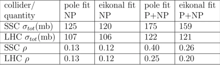
is comfortably perturbative, we pick a value of 2 GeV, and we show the resulting curves in Figure 3 and their eikonalized version in Figure 4. The predictions for the LHC and the SSC are given in table 1.
collider/ pole fit eikonal fit pole fit eikonal fit
quantity NP NP P+NP P+NP
SSC σtot(mb) 125 120 175 159
LHC σtot(mb) 107 106 122 121
SSC ρ 0.13 0.12 0.40 0.26
LHC ρ 0.13 0.12 0.25 0.20
Table 1: Allowed values of the cross section and the ρ parameter. The first two columns result from the purely non-perturbative (NP) ansatz (1), and the two last columns (P+NP) from its perturbative evolution, with Q0 = 2
GeV, see equation (9).
Clearly, unitarization is not going to make a big difference even at SSC energies. Its main effect will be to bring down the ρ parameter at ultra high
energy √s ≈ 105 GeV. One sees from these curves that the perturbative
component could contribute 50 mb (15 mb) at the SSC (LHC). We emphasize that this is a conservative estimate, based on an infrared cutoff of 2 GeV. Cutting off the evolution when αS ≈ 1 would give a total cross section of at
least 3 b at the SSC, and be consistent with all available collider and fixed target data!
5
Conclusion
We have shown that the BFKL equation can be used to evolve the soft pomeron to higher s, and that perturbative effects could become measur-able at the SSC/LHC. These effects are cutoff dependent, and perturbative physics seems to couple very weakly to the proton in the diffractive region, its coupling strength being a few percent of that of the soft pomeron. However, even a very weak coupling turning on at an energy of a few GeV can lead to measurable effects at sufficiently large energy. It is known that the pomeron couples to quarks, and quarks to gluons. The coupling to the BFKL ladder thus cannot be zero, and specific models can be built for it [14].
This contribution is genuinely new and comes entirely from a QCD anal-ysis. One should not be mislead by previous parton models [5] which, while using a partonic picture, keep it mostly non-perturbative, replacing the small power sǫ0 of (1) by a small power x−ǫ0 in the gluon structure function xg(x). In the present model, xg(x) will contain the same powers ǫi(Q0/x) as the
to-tal cross section, but their coefficients will in general be different from those entering the total cross section, and the relation between them will be model dependent.
The existence of such possibilities, and the fact that very large total cross sections are expected from the same kind of arguments that lead one to predict a rising cross section [13, 15], shows that small momentum physics contains a wealth of open possibilities worth exploring experimentally.
Acknowledgments
This work was supported in part by NSERC (Canada) and les fonds FCAR (Qu´ebec).
References
[1] A. Bialas and P.V. Landshoff, Phys. Lett. B256, 540 (1991)
[2] J.D. Bjorken, preprint SLAC-PUB-5545 (May 1991), SLAC-PUB-5616 (March 1992)
[3] A. Donnachie and P.V. Landshoff, Nucl. Phys. B267, 690 (1986); Nucl. Phys. B231, 189 (1984)
[4] C. Bourelly, J. Soffer and T.T. Wu, Mod. Phys. Lett. A6, 2973 (1991) [5] M.M. Block, F. Halzen and B. Margolis, Phys. Rev. D45, 839 (1992) [6] R.E. Hancock and D.A. Ross, preprint SHEP 91/92-14 (1992)
[7] E.A. Kuraev, L.N. Lipatov and V.S. Fadin, Sov. Phys. JETP 44, 443 (1976) and 45, 199 (1977); Ya Ya Balitskii and L.N. Lipatov, Sov. J. Nucl. Phys. 28, 822 (1978)
[8] E-710 Collab., presented at the International Conference on Elastic and Diffractive Scattering (4th Blois Workshop), Elba, Italy, May 22, 1991, to be published in Nucl. Phys. B (Proc. Suppl.) B25 (1992); CDF Col-lab., same proceedings; M. Bozzo et al., Phys. Lett. 147B, 392; M. Ambrosio et al., Phys. Lett. 115B, 495 (1982); N. Amos et al., Phys. Lett. 120B, 460 (1983); 128B, 343 (1984); U. Amaldi and K.R. Schu-bert, Nucl. Phys. B166, 301 (1980)
[9] L.N. Lipatov, Sov. Phys. JETP 63, 904 (1986); R. Kirschner and L.N. Lipatov, Zeit. Phys. C45, 477 (1990)
[10] G.J. Daniell and D.A. Ross, Phys. Lett. 224B, 166 (1989) [11] J.C. Collins and J. Kwiecinski, Nucl. Phys. B316, 307 (1989) [12] J.C. Collins and P.V. Landshoff, Phys. Lett. 276B, 196 (1992) [13] S. Frautschi and B. Margolis, Nuov. Cim. 57A, 427 (1968) [14] J.R. Cudell, work in progress.
[15] W. Heisenberg, in Kosmiche Strahlung (Springer-Verlag, Berlin:1953), p. 148; V. Gribov and A. Migdal, Sov. J. Nucl. Phys. 8, 583 (1969); N. W. Dean, Phys. Rev. 182, 1695 (1969); H. Cheng and T.T. Wu, Phys. Rev. Lett. 24, 1456 (1970); S.T. Sukhorukov and K.A. Ter-Martirosyan, Phys. Lett. 41B, 618 (1972)
Figure Captions
Figure 1: Simple pole fit (1) at zero momentum transfer, for pp and p¯p scattering, as indicated. (a) shows the total cross section and (b) the ratio of the real-to-imaginary parts of the amplitude. The data are from reference [8].
Figure 2: (a) shows the effective power of s of equation (9) that results from a cutoff BFKL equation, for various values of the infrared cutoff Q0, as
indicated next to the curves. (b) gives the 2σ allowed regions for an amplitude given by equation (9) (hatched region) or eikonalized (cross hatched). The abscissa is the infrared cutoff Q0 and the ordinate the ratio of the coupling
strength of the perturbative ladder to that of the soft pomeron.
Figure 3: same as figure 1. The upper curve shows the maximum values of the cross-section (a) and of ρ (b) that might result from a perturbative evolution consistent with all present data.