The Transparent Dead Leaves Model
Texte intégral
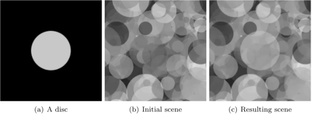
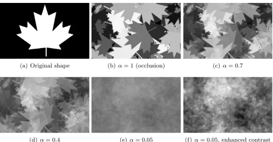
Figure

Documents relatifs
From the empirical results and the simulation experiments, we draw the conclusion that the proposed portmanteau test based on squared residuals of an APGARCH(p, q) (when the power
Abstract: This paper presents a digital holographic method to visualize and measure refractive index variations, convection currents, or thermal gradients,
This evolution between the standard Gaussian models to non-Gaussian ones is not a surprise since an ever- growing number of experimental measures has highlighted
When applied to the man- agement of the data used and produced by applications, this principle means that the grid infrastructure should automatically handle data storage and
That view proved to lack accuracy, and our color representation now tries to estimate both a global color model, that separates leaf pixels from background pixels, and a local
DEFORMABLE COMPOUND LEAF MODELS Similarly to what we have done in the case of simple leaves [11], the segmentation method we propose relies on the prior evaluation of a flexible
Data management (persistent storage, transfer, consistent replication) is totally delegated to the service, whereas the applications simply access shared data via global
Data management (persistent storage, transfer, consistent replication) is totally delegated to the service, whereas the applications simply access shared data via global
