Université de Neuchâtel Institut de Géologie
Formation and transport of CH
4
and CO
2
in deep peatlands
Isotope geochemical analysis and numerical modelling
based on field research at the
Etang de la Gruère Bog in Switzerland
Thèse
Présentée à la Faculté des Sciences de l’Université de Neuchâtel (Suisse)
pour l’obtention du grade de
Docteur ès Sciences
par
B
ERNDE
ILRICH2002
Jury:
PROF. KARL B. FÖLLMI (Neuchâtel) directeur de thèse
DR. PHILIPP STEINMANN (Neuchâtel) co-directeur de thèse
PROF. STEPHEN J. BURNS (Amherst, Massachusetts)
PROF. JEAN-MICHEL GOBAT (Neuchâtel)
TABLE OF CONTENTS
1 FOREWORD ... 7
1.1 STRUCTURE OF THIS MANUSCRIPT... 7
1.2 CONTEXT OF THIS WORK... 7
1.3 FINANCIAL SUPPORT... 7
2 INTRODUCTION ... 9
2.1 OMBROTROPHIC AND MINEROTROPHIC MIRES... 9
2.2 OCCURRENCE OF PEATLANDS IN GENERAL … ... 10
2.3 ACROTELM AND CATOTELM... 12
2.4 GEOCHEMISTRY OF OMBROTROPHIC MIRES... 12
2.5 PRINCIPAL PHYSICAL TRANSPORT PROCESSES OF CHEMICAL SPECIES IN BOG PORE WATER... 14
2.5.1 Pore water advection ... 14
2.5.2 Molecular diffusion ... 14
2.5.3 Ebullition... 15
2.6 PEATLANDS AND GREENHOUSE GAS EMISSION... 16
2.7 METHANE EMISSIONS FROM PEATLANDS... 18
2.8 HOW DOES METHANE FORM IN PEATLANDS? ... 19
3 THE STUDY SITES... 21
3.1 ETANG DE LA GRUÈRE (EGR) ... 21
3.1.1 Physiographical setting... 22
3.1.2 Geological setting ... 23
3.1.3 Climate ... 24
3.1.4 Peat characteristics... 24
3.2 Other field sites ... 26
4 METHODS... 27
4.1 SAMPLING OF BOG PORE WATERS... 27
4.2 MEASUREMENTS OF THE PHYSICAL PROPERTIES OF THE EGR PORE WATER... 31
4.2.1 Temperature ... 31
4.2.1.1 Manual temperature measurements ... 31
4.2.1.2 Automatic temperature recording... 33
4.2.2 Water level and vertical hydraulic gradient ... 33
4.3 CHEMICAL ANALYSIS OF BOG PORE WATERS... 34
4.3.1 Determination of pH... 34
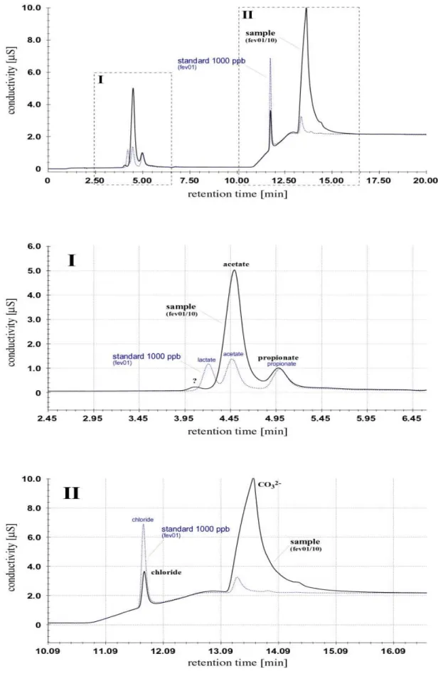
4.3.2 Ion chromatography of organic-rich waters from peatlands... 34
4.3.2.1 Anions... 35
4.3.2.2 Cations ... 38
4.3.3 Gas chromatography and headspace gas analysis ... 41
4.3.3.1 Method... 41
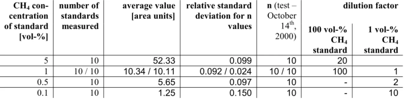
4.3.3.2 Calibration ... 41
4.3.3.3 Blanks ... 43
4.3.3.4 Duplicates ... 43
4.3.3.6 Calculation of the CH4 concentration from headspace gas analysis ... 45
4.3.4 Dissolved organic carbon ... 46
4.4 MASS-SPECTROMETRY OF CARBON STABLE ISOTOPES... 47
4.4.1 Sample preparation and storage (Pore water methane and DIC) ... 48
4.4.2 Pore water CH4 carbon stable isotope analysis... 48
4.4.3 DIC carbon stable isotope analysis ... 49
4.4.4 Pore water DOC carbon stable isotope - sample preparation and storage ... 49
4.4.5 Separation of humic and fulvic acids ... 50
4.4.6 Carbon stable isotope analysis of separated humic and fulvic acids ... 50
4.4.7 CO2 and CH4 carbon stable isotope analysis of gas emissions ... 50
4.4.8 Peat matrix carbon stable isotope analysis... 50
4.5 SAMPLING OF GAS ON THE BOG SITE... 51
4.5.1 Preparation of the field site... 51
4.5.1.1 Receptacles ... 52
4.5.1.2 Purging of the receptacles... 52
4.5.2 Gas sampling... 53 4.6 GAS FLUX MEASUREMENTS... 53 4.6.1 CO2... 53 4.6.2 CH4... 54 4.6.2.1 Method... 55 4.6.2.2 Calibration ... 55 4.6.2.3 Blanks ... 56 4.6.2.4 Corrections... 56
5 HYDROLOGY AND MAJOR ELEMENTS ... 59
5.1 MAJOR ELEMENT CONCENTRATIONS AND THEIR SEASONAL VARIATIONS... 59
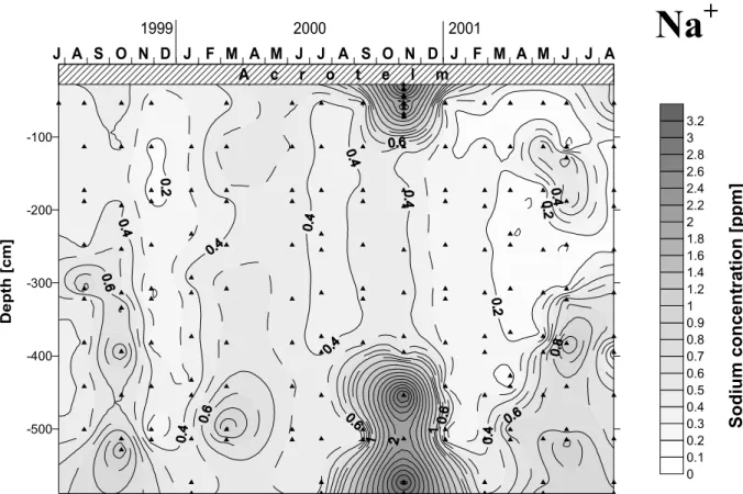
5.1.1 Sodium (Na+)... 60
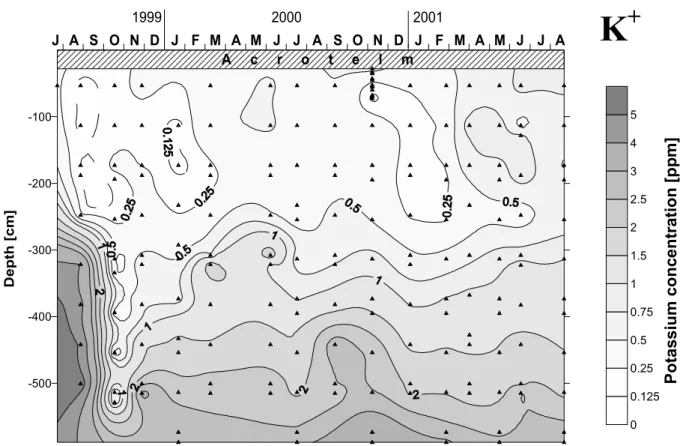
5.1.2 Potassium (K+) ... 60
5.1.3 Magnesium (Mg2+) ... 62
5.1.4 Calcium (Ca2+)... 62
5.1.5 Early phase of sampling - potassium, magnesium, calcium ... 63
5.1.6 Ammonium (NH4+) ... 63
5.1.7 Chloride (Cl-) ... 64
5.1.8 Dissolved inorganic carbon (H2CO3*, HCO3-, CO32-)... 65
5.1.9 November 2000 data from a different peeper (Type A) ... 67
5.2 PHYSIOCHEMICAL, PHYSICAL, AND HYDROLOGICAL CHARACTERISTICS... 68
5.2.1 pH ... 68
5.2.2 Precipitation and temperature ... 70
5.2.3 Water table ... 72
5.2.4 Piezometer data... 73
5.2.5 Other hydrological observations at EGr... 74
5.2.6 Pore water temperature ... 75
6 METHANE AND CO2 IN PEATLANDS - IMPLICATIONS FROM EGR DATA 77 6.1 ACETATE IN DEEP PEAT BOG ENVIRONMENTS - SEASONAL VARIATION AND IMPLICATIONS FOR METHANOGENESIS: INVESTIGATION OF AN OMBROTROPHIC PEAT BOG IN THE JURA MOUNTAINS, SWITZERLAND (PAPER IN PREPARATION) ... 77
6.1.1 Abstract ... 77
6.1.2 Introduction... 77
6.1.4 Methods ... 79
6.1.5 Results ... 80
6.1.6 Discussion ... 82
6.1.7 Conclusions ... 85
6.2 PATHWAYS OF METHANOGENESIS IN PEATLANDS: ACETATE SPLITTING VS. CO2 REDUCTION - IMPLICATIONS FROM CARBON STABLE ISOTOPE DATA (PAPER IN PREPARATION).. ... 86
6.2.1 Abstract ... 86
6.2.2 Introduction... 86
6.2.3 Methods ... 88
6.2.3.1 Pore water sampling ... 88
6.2.3.2 Methane carbon stable isotope analysis... 88
6.2.3.3 DIC carbon stable isotope analysis... 88
6.2.3.4 Methane concentration analysis... 88
6.2.4 Results ... 88
6.2.4.1 d 13C-CH 4... 88
6.2.4.2 d 13C-DIC... 89
6.2.4.3 d 13C-DOC ... 90
6.2.4.4 d 13C of humic and fulvic acids... 90
6.2.5 Discussion ... 91
6.2.5.1 Depth dependent “static” patterns ... 94
6.2.5.2 Seasonal “dynamic” patterns ... 95
6.2.5.3 d 13C-DIC... 96
6.2.5.4 Isotope fractionation and organic matter ... 97
6.2.6 Conclusions ... 98
6.3 OBSERVATIONS ON THE INFLUENCE OF OTHER SPECIES... 98
6.4 A MODEL OF METHANE AND CO2 PRODUCTION AND TRANSPORT IN DEEP PEATLANDS - IMPLICATIONS FOR GREENHOUSE GAS EMISSIONS (PAPER IN PREPARATION)... 101
6.4.1 Abstract ... 101
6.4.2 Introduction... 101
6.4.2.1 The model: Purpose and concept... 102
6.4.2.2 Realisation ... 103
6.4.2.3 Model parameters ... 104
6.4.2.4 Diffusive species transport ... 104
6.4.2.5 Bubble formation and ebullition... 105
6.4.2.6 Gas over-saturation of the pore water... 105
6.4.2.7 Methane and CO2 production in the catotelm ... 105
6.4.2.8 DIC vs. CO2... 106
6.4.2.9 pH gradient ... 106
6.4.2.10 Calculation time interval ... 106
6.4.2.11 Methane carbon stable isotopes... 107
6.4.3 Results ... 107
6.4.3.1 Modelled methane, DIC, and N2 concentrations ... 107
6.4.3.2 Diffusion vs. bubble formation... 108
6.4.3.3 Diffusion vs. advection... 108
6.4.3.4 Bubble composition... 108
6.4.3.5 Carbon stable isotope characteristics for pore water methane ... 110
6.4.4 Discussion ... 110
6.4.4.1 Methane and DIC concentrations ... 110
6.4.4.3 Influence of pore water over-saturation... 111
6.4.4.4 Influence of pH... 112
6.4.4.5 Calculated methane emissions... 112
6.4.4.6 Agreement of the model results... 112
6.4.5 Conclusions ... 113
7 GENERAL CONCLUSIONS ... 115
8 SUMMARY... 117
8.1 ENGLISH VERSION... 117
8.2 RÉSUMÉ EN FRANÇAIS (FRENCH VERSION)... 118
8.3 ZUSAMMENFASSUNG AUF DEUTSCH (GERMAN VERSION) ... 119
9 ACKNOWLEDGEMENTS ... 121
10 REFERENCES ... 125
11 APPENDICES ... 135
© B. Eilrich, 2002 All rights reserved.
1 FOREWORD
1.1 Structure of this manuscript
The main results of research are presented in three papers, which constitute the body of this thesis. They focus on the pore water geochemistry of the Etang de la Gruère Bog and on its implications for microbial methanogenic pathways and gas transport in peatlands.
An introductory chapter (2) states the objective of this study and explains the significance of peatland carbon mineralisation and methanogenesis. Current developments in this field of research are briefly reviewed to address the open questions. The following chapters reflect the course of the investigation with fieldwork, laboratory analysis, modelling and interpretation. The field site with its geological and climatological characteristics is presented in chapter 3.
Chapter 4 describes the methods applied in the field and in the laboratory. Particular
emphasis is put on those methods and instruments, which have especially been designed or adapted for deep peat pore water research and have been used by the author of this study. Results, which have not been included in the papers, are presented in chapter 5.
The three papers bear the most important outcome of this study. They are incorporated in
chapter 6 and appear in a non-finalised version. Some information may occur more than one
time, especially in the introductions and discussions. Some general conclusions (chapter 7) are intended to bring the various implications of these three studies together and indicate, where further research is needed. The summary of this thesis, given in chapter 8 in English, French and German language, is followed by the acknowledgements and references (chapters
9 and 10). Tables containing analytical data and additional information are provided in the
appendices.
1.2 Context of this work
A wide range of biological, geochemical and hydrological issues have already been studied at the Etang de la Gruère, one of Switzerland’s largest remaining peat bogs. Among other scientists, the main applicant for this research project (P. Steinmann, Neuchâtel University) investigated the Etang de la Gruère for his PhD thesis. Dr. Steinmann’s studies focussed on the geochemistry of peat and pore water. The here presented research can be seen as a continuation of his work, broadening certain aspects of peat pore water chemistry and addressing new questions, while inevitably neglecting others. It represents a pluridisciplinary approach involving partners from the Geochemical and Environmental Analysis Group at the Geological Institute and the Microbiology Laboratory at the Botanical Institute of Neuchâtel University as well as the Stable Isotope Laboratories of the Geological Institute and of the Division of Climate and Environmental Physics at the Physics Institute of Bern University.
1.3 Financial support
This research project has been funded by the Swiss National Sciences Foundation (SNF), grants nos. 21-55630.98 and 20-63841.00. A 12.5 % assistant position within the Institute of Geology has been made available to the author since February 2000. The IGBP poster award on the occasion of the “First Swiss Global Change Day” helped financing the author’s participation at the Goldschmidt 2000 Conference in Oxford, UK.
2 INTRODUCTION
This study deals with peatland geochemistry. It is based on field research at the Etang de la Gruère Bog (EGr) in Switzerland and focuses on methane (CH4) and carbon dioxide (CO2)
formation and transport in the lower peat layers, the so-called catotelm. Both CO2 and
methane are important greenhouse gases.
2.1 Ombrotrophic and minerotrophic mires
Bogs such as EGr receive their water and nutrient supply solely from the atmosphere
(precipitation, dust). They are also referred to as “ombrotrophic” or “ombrogenous” mires (gr. ombros = rain). Fen peats, by contrast, are predominantly fed by mineral-rich water, e.g. ground water or river water, and are therefore sometimes named “minerotrophic” or “minerogenous” mires. Table 2-1 summarises the similarity and differences of these two major peatland types.
Table 2-1: Summary of major bog and fen characteristics according to Maltby and Proctor (1997) and IPCC
(1996).
Bogs can further be subdivided into two different types, blanket bogs and raised bogs (Fig. 2-1). Blanket bogs extend over the landscape like a blanket and consist of relatively thin peat, which follows the underlying topography. Raised bogs such as the EGr are gently domed areas of acid peat, which develop typically over fen peats of filled-in lake basins, over coastal flats or river floodplains (Maltby and Proctor, 1997). It is interesting to note that by weight, a raised bog in its upper fresh part may be up to 98 % water and only 2 % solid peat1 (IPCC, 1996). Blanket bogs are rather more solid with up to 85 % water.2
fen peat (minerotrophic) bog (ombrotrophic)
habitat waterlogged waterlogged
water and solute
supply predominantly ground water atmospheric input
average depth generally <2 m between 2 and 12 m in most cases
mineral content relatively high very low
ash content high (10 % and more) low (ca. 3 %)
pH in near surface pore waters
7 - 8 3 - 4.5
C : N ratio <20 >30
C : P ratio <100 in most cases >1000 in most cases
Fig. 2-1: Schematic illustration of the two major bog types.
Type A corresponds to the investigated convex-shape part of the Etang de la Gruère Bog and may reach a thickness of several meters. Type B is relatively thin (<1 m in most cases) and much more frequent at low altitudes. So-called “Atlantic blanket bogs” below 200 m asl. are distinguished from “mountain blanket bogs” above 200 m asl. (according to IPCC, 1996).
1 A raised peat bog may hence contain fewer solids than, for example, milk.
2 This great volume of water is held within the dead Sphagnum fragments. The ability to retain water is one of
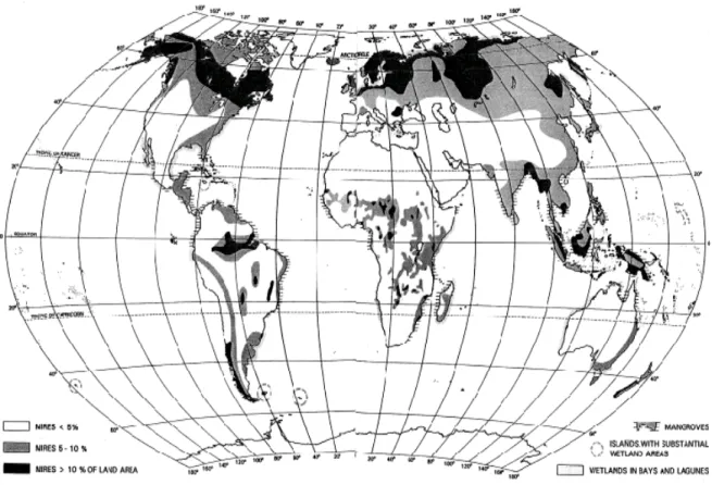
2.2 Occurrence of peatlands
in general …Fig. 2-2: Map showing the global distribution of peatlands (mires with a minimum peat thickness of 30 cm;
according to Lappalainen, 1997). In this figure, however, the percentage of remaining peatlands in northern Central Europe is overestimated (K. Föllmi - pers. comm.).
Fig. 2-2 shows the global distribution of “peatlands” in a wide sense, i.e. including also marshlands, gleysols, tundra soils, fluvisols and other histosols (peat soils), yet, no swamps are included, such as those at the mouths of the rivers Guadalquivir in Spain and Nile in Egypt. A map showing the location of important mires in Switzerland is given in Fig. 2-3. Estimates of the total area of the World’s peatlands (bogs and fens only) vary considerably from about 1.1 (Bülow, 1929; Nikonow and Sluka, 1964) and ca. 5 (Kivinen and Pakarinen, 1981) to 6 million km2 (Maltby, 1988). One reason for this large variation is certainly the age of the estimates and the problems encountered when doing such a global survey (lack of detailed information about remote areas, use and availability of survey methods, e.g. aerial and satellite imagery). Another reason is the still ongoing loss of peatlands, e.g. by transformation in agricultural soils (e.g. Dungan, 1990; Inisheva 2000). The basic problem, however, is to distinguish areas where the peat layer is 30 cm at minimum from areas just covered by wetland vegetation (floodplains, coastal lagoons, mangroves, swamps). On this basis, a detailed and more recent analysis is provided by Lappalainen (1997), who estimated the global peatland area at 3,985,000 km2. This area represents about 3 % of the Earth’s total ice-free land surface. The global peatlands contain some 5 to 6*1012 t of wet peat (Lappalainen, 1997).
Fig. 2-3: Distribution of
mires of national
importance in Switzerland (according to Küttel, 1997). 1 - Vallée de Sagne; 2 - Along the southeastern shore of Lake Neuchâtel; 3 - Franches Montagnes; 4 - Berner Oberland and central Switzerland north of Lake Thun and Lake Brienz.
… and of ombrotrophic mires in particular
As ombrotrophic mires (bogs) are entirely dependent on atmospheric input for their water and nutrient supply, they only develop in humid regions without seasonally too pronounced deficits in precipitation3. Hence they occur predominantly in temperate latitudes (generally between 50 to 70° N, in mountainous regions also further south) in Europe, Asia, western North America and somewhat further south in eastern North America (Maltby and Proctor, 1997; Malterer, 1997; Rubec, 1997). Along with fen peats, these ombrotrophic mires are often referred to as “northern hemisphere peatlands” (e.g. Fung, et al., 1991), because their occurrence is very much restricted in the southern hemisphere due to the absence of landmass in the corresponding latitudes.4 The northern limit for accumulation of deep peat in ombrotrophic mires is probably set by declining primary production and longer frost periods at high latitudes. The extensive subarctic and low-arctic peatlands are generally shallower, more acidic and nutrient-poor (Gore, 1983; Whigham et al., 1993). The southern and eastern limits of northern hemisphere peatlands are probably determined by the maximum tolerable summer water deficit, at which net accumulation of peat can take place (Maltby and Proctor, 1997). An example for huge northern hemisphere peatlands is the west Siberian Great Vasjugan Bog (cf. Fig. 3-7), from which pore water samples have been obtained in the course of this study (cf. chapters 3.2, 11.AI-3, and 11.AII-14). The Great Vasjugan Bog is the world’s largest coherent mire. It covers an area of more than 50,000 km2 (Inisheva et al., 2000).
Ombrotrophic mires do also occur in tropical regions, e.g. in Amazonia, Equatorial Africa and Southeast Asia (Fig. 2-2). Tropical bogs are primarily distinct from northern peatlands by vegetation. Usually, they are tree-covered, their pore water chemistry and ash (non-organic matter) content, however, clearly indicate ombrotrophic origin. Domed bogs, e.g. near Riau on the Indonesian island of Sumatra, may reach 10 m or more of peat thickness (Rieley et al., 1997).
3 In turn, carbon isotopes in bog plants may be used as climatic indicators (Ménot and Burns, 2001).
4 Some smaller peatlands, however, can be found on the South Island of New Zealand (Dobson, 1979), the
2.3 Acrotelm and catotelm
Each bog reveals its individual peat stratigraphy (layering) with specific characteristics for the fibric matrix, the degree of decomposition and compaction, the hydraulic conductivity, the ash (i.e. non-organic matter) content, and so forth. Despite the multitude of individual characteristics, two principal zones are usually common to all bogs. The upper zone is called the acrotelm or the root-zone5. The acrotelm is a thin layer, generally only some 30 cm deep. It consists of fibres of predominantly Sphagnum (e.g. Sphagnum fuscum, Sphagnum magellanicum) mosses, which are largely still alive, often in upright position and colourful with red, yellows and ochre. Rainwater can move relatively rapidly through this layer. The water level and the degree of oxygenation in this zone are subject to seasonal change. The zone below the acrotelm comprising the bulk of the peat and reaching to the ground of the bog is known as the catotelm. The catotelm is generally much thicker than the acrotelm and always water-saturated. It consists of often significantly decomposed peat, where individual plant stems have collapsed under the weight of mosses above them and have produced an amorphous, dark-coloured fibric mass of plant fragments. Water movement through this amorphous peat is slow - typically much less than 0.1 m per day (IPCC, 1996). In consequence of water saturation and organic matter decomposition, the catotelm is permanently anaerobic.
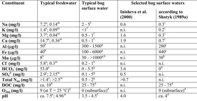
2.4 Geochemistry of ombrotrophic mires
Ombrotrophic mires are extremely low in nutritive elements. This is a direct consequence of the conditions of formation and particularly true for nitrogen (N) and phosphorus (P); cf. Table 2-1. Aerts et al. (1992) showed that in natural remote bogs N is limiting to plant growth, while in bogs closer to areas, which are more influenced by human activity and predominantly by agriculture, the limiting nutritive element is P.
Potassium (K) is another major nutrient for plants and animals and also tightly cycled. Typically, K concentrations are highest in the active vegetation zone at the top of the bog. Absolute concentrations, however, are low (<1 mg*l-1, cf. Table 2-2) and fluctuate more widely during the seasons and from bog to bog than other major elements such as sodium (Na), magnesium (Mg), and calcium (Ca) (Maltby and Proctor, 1997). As can be inferred from Table 2-2, the concentrations of all major elements are very variable from place to place, although the absolute concentrations are small compared to other fresh water systems. Due to low pH as well as abundant dissolved organic matter (and hence increased solubility and complexation), bog waters are enriched in elements like aluminium (Al), manganese (Mn) and iron (Fe) relative to “normal” freshwaters (Ramann, 1895; Shotyk, 1997). The relative abundance of Fe in mire surface waters is often apparent as iridescent, ‘oily’ film of chalybeate (‘containing iron’) waters, which have come in contact with air (cf. Shotyk, 1988). This phenomenon has been reported in numerous publications (e.g. Dachnowski, 1912; Puustjärvi, 1952, Armstrong and Boatman, 1967).
5 The term “root-zone” is misleading, because in strict biological sense Sphagnum mosses, which are the most
important plant species in raised mires, do not have roots. Their stems continue to grow at the surface during peat accumulation and may be as long as 30 - 40 cm below the surface. Alike other typical peatland plants, they have well developed aerenchyma, allowing oxygen to diffuse down from the above ground parts (Crum, 1984). An example for a widespread bog plant with roots is Eriophorum.
In near surface bog waters, chloride, bicarbonate, and sulphate6 are the major inorganic anions (Maltby and Proctor, 1997). Some 10 to 30 %7 of the total anion charge is accounted for by the dissolved organic matter, e.g. humic, fulvic, or carboxylic acids (Maltby and Proctor, 1997). Most investigations show low but relative constant chloride concentrations in the order of 0.2 - 1 mg*l-1 (Steinmann and Shotyk, 1997a, Wind-Mulder and Vitt, 2000). Chloride concentrations in peat bogs can be up to 10 times higher than in rainwater because of mixing of the bog pore water with nearby ground waters (Steinmann and Shotyk, 1994; cf. Table 2-2). Below the acrotelm, nitrate (NO3-), sulphate (SO42-) and phosphate (PO43-) concentrations
are rapidly diminishing to virtually zero, yet may again increase towards the ground (Brown, 1985; Steinmann, 1995). There is no general rule for the concentration change in the peat bog profile. While the Mn concentration is usually decreasing with depth (Shotyk, 1986) due to precipitation at the top under less reducing conditions (“redox recycling”), the Mg and Ca concentrations are generally increasing with depth (e.g. Steinmann, 1995). At EGr, the average concentration increase from pore waters at 0.5 m depth to pore waters at 5 m depth, is about 2 fold for Na, 5 fold for K, 50 fold for Ca, and 100 fold for Mg (cf. chapter 5.1). The main reason for this concentration increase is an increased influence of the substratum (clays and marls at EGr; cf. chapter 3.1.2) on the bog pore water chemistry.
Moreover, at the time when the deeper peat layers formed, these were situated much closer to the substratum and in touch with mineral rich ground waters (“fen peat”, cf. chapter 2.1). Peat layers in the lower bog may therefore still show “fen conditions” (Shotyk et al., 2001) and continue to be an ion source for the peat pore water. The groundwater represents another important source, from which ions may derive by mixing and diffusion (McKenzie et al., 2002).
Table 2-2: Chemical composition of bog surface waters versus typical freshwaters (modified from Shotyk,
1989a).
Selected bog surface waters
Constituent Typical freshwater Typical bog
surface water
Inisheva et al.
(2000) according to Shotyk (1989a)
Na (mg/l) 7.2a; 0.14m 2 - 5f 0.6 0.3i K (mg/l) 1.4a; 0.09m <1f n.i. 0.2i Mg (mg/l) 3.7a; 0.04m 0.5 - 1f 1.6 0.3i Ca (mg/l) 14.7a; 0.36m 0.5 - 1f 1.9 0.7i Al (mg/l) 50b 300 - 1500g n.i. 280j Fe (mg/l) 40b 100 - 6000g n.i. 440j Mn (mg/l) 8b 30 - >1000g,h n.i. 30h Cl- (mg/l) 5.8a; 0.3m 0.2 - 1k n.i. n.i. HCO3- (mg/l) 53.0a 0 - 5.5g 3.6 0d SO42- (mg/l) 2.9c; 2.15m 0.1 - 5g 0.5 n.i. Total Naq (mg/l) >1.4c; >2.5m 0.5 - 2g >0.7 n.i.
DOC (mg/l) ca. 10d 25 - 75d n.i. 25 - 75d
O2aq (mg/l) 9 (at T = 25 °C)d 0 (subsurface)d n.i. 0 (subsurface)d
pH ca. 7.5e; 4.96m 3.5 - 4.5f 4.0 ca. 4d
6 The sulphate concentrations in bog pore waters are however often overestimated as a consequence of organic
sulphide oxidation in the sample. Sulphate concentration analysis carried out directly after sampling for this study showed only minor (<150 ppb) concentrations, which declined rapidly with depth (cf. chapter 11.AII).
7 Oxidation effects during sample taking and storage potentially lead to an overestimation of the sulphate
concentration and may, in turn, cause an underestimation of the dissolved organic matter concentration. The analysis of bog pore water sampled with particular care (e.g. sampling under a nitrogen atmosphere) demonstrated that the share of dissolved organic matter in the total anion charge could be as high as 80 % (Steinmann and Shotyk, 1997a).
a World average river water (Berner and Berner, 1987) b Typical freshwater composition (Drever, 1997) c Likens et al. (1977) in Drever (1982)
d Shotyk (1989) e Calculated from [HCO
3-] assuming pCO2 = 10-3.0 bar f Maltby and Proctor (1987)
g Shotyk (1988) h Shotyk (1987) i Gorham et al. (1985) j Urban et al. (1987)
k Wind-Mulder and Witt (2000)
m Average chemical composition of wet deposition at Payerne, 1985-1991
(EMPA 1985-1991; in Steinmann and Shotyk, 1994) n.i. not indicated
2.5 Principal physical transport processes of chemical
species in bog pore water
2.5.1 Pore water advection
Advection is defined as the bulk movement of a fluid, e.g. due to pressure or density contrasts
(Krauskopf and Bird, 1995). In hydrogeology, advection is often associated with the transport of a non-reactive, conservative contaminant, or tracer, in a porous medium at a velocity equal to the average groundwater velocity (Piteau Associates, 1993). For peatlands, the term advection has a slightly different meaning: When rainwater falls on a bog or when snow and ice melt, the water at the surface increases the hydrostatic pressure in the pore water column and the water will start to flow downwards (and to a certain degree also sidewards) through the permeable pore space until a new hydrostatic equilibrium is attained. The flow field is determined by the hydraulic gradients and the hydraulic conductivities. The downward flow of water through the pores is called pore water advection. Advective species transport in peat bogs is usually unidirectional from up to down. There are however important exceptions, where transport is upward directed due to pore water tension (e.g. Siegel et al., 1995). The location in the bog (a central location, for example, or near the margins), the degree of curvature of the raised part of the bog, and hydrological parameters such as the ratio of the vertical and the horizontal hydraulic conductivity, determine how much water will flow downwards and to the sides (cf. chapter 5.2.5 and Fig. 5-16). Individual and very complex flow direction may occur in every bog.
When pore water moves down due to advection, its chemical load (ions, colloids, dissolved gas) is also transported to greater depths. The rate of pore water advection depends primarily on the amount of precipitation, the peat’s hydraulic conductivity, permeability, thickness, as well as the bog’s lateral extension and its confinements, which may be more or less watertight. Pore water temperature patterns at EGr (cf. chapter 5.2.2 and Fig. 5-17) indicate pore water advection rates of about 1 to 3 cm per day.
2.5.2 Molecular diffusion
Diffusion is defined as the intermixing of atoms and/or molecules of solids, liquids and gases,
where the atoms or molecules of a certain type move from an area of high concentration to an area of low concentration (Vogt and Wargo, 1993). Fick’s first law describes the rate of
diffusion of a substance across a surface element, as given by a formula expressing the proportionality between diffusion flux J [mol*m*s-1] and concentration gradient dC/dx. In this equation, J = -D dC/dx, where D [m2*s-1] is the diffusion coefficient (Harcourt, 2002). Fick’s first law is often used to quantify the diffusive flux of molecules in liquid systems (e.g. Makhov and Bazhin, 1999). Most dissolved gases such as sulphur hexafluoride (SF6) and
methane, are transported by molecular diffusion (Van Bodegom et al., 2001; Van Bodegom and Scholten, 2001), while for other gases, such as CO2 (“carbonate equilibrium”), ion
diffusion plays an important or, as for instance in the case of hydrochloric acid gas (HCl), virtually the only role. For ion diffusion, the charge balance should also be considered (cf. chapter 4.3.2). In a technical sense, peatlands can be regarded as a suspension of solid matter (the peat matrix) in water. In contrast to advection, which is restricted to relatively large interconnected pore space, diffusion also occurs in fine pore space. It is hence much more influenced by molecule-scale electrostatic effects as in “open” media. For a more exact estimate of diffusive transport in porous media, again, the charge balance should also be taken into account (cf. Steinmann, 1995).
2.5.3 Ebullition
Gas species in peatlands may also be transported in the gas phase by bubbles. In theory, bubbles form, when the pressure of all gas species dissolved in the pore water (i.e. the sum of their partial pressures) exceeds the confining hydrostatic pressure. In practice, this is not always the case (see below). The relationship between the concentration of a dissolved gas species and its corresponding partial pressure is given by Henry’s law, which states that the pressure in a co-existing gas phase is directly proportional to the concentration of the gas in the solution (Harcourt, 2002). The equilibrium constant (“Henry’s law constant”) KH [M*bar -1) = C(gas)/p(gas), where C(gas) is the concentration of this gas in solution and p(gas) is the
partial pressure of an ideal gas. Sander (1999) provides a comprehensive list of Henry constants for numerous chemical compounds. Bubble formation and transport are commonly described as ebullition. As it is generally the case for advection, ebullitive species transport is unidirectional. Yet in contrast to the latter, it is upward directed due to the buoyancy of gas bubbles in water.
Often, a considerable over-saturation of the pore water with gas species occurs (Abegg and Anderson, 1997; Siegel et al., 1997). This means that the total partial pressure of the dissolved gas species exceeds the confining hydrostatic pressure without bubble formation. Gas over-saturation is particularly pronounced in porous media (e.g. in the lower catotelm of EGr up to 1.8 times; cf. chapter 6.4.4.3 and chapter 11.AIII-Goldschmidt’00-Fig.2a), where the pore walls impede bubble growth. The bubble formation in porous media is very complex and many factors (e.g. the maximum possible bubble size, effects of surface tension, replacement of the liquid by gas, re-equilibration of the gas content during bubble movement) need to be taken into account (cf. Chanton et al., 1989b). In laboratory experiments (incubation of peat soils) carried out by Lansdown et al. (1992), the ebullitive flux of methane was more than 15 times larger than the diffusive flux.
2.6 Peatlands and greenhouse gas emission
Greenhouse gas emissions to the atmosphere and concentration variations are often seen in relation to human activity (Table 2-3). For the global greenhouse gas budget however, natural emissions, in particular of CO2 and CH4, are very important. In case of CH4, peatlands
represent the largest single natural source (Fig. 2-4) - cf. chapters 2.6 and 2.7.
Table 2-3: Examples of greenhouse gases that are affected by human activities (according to IPCC, 2001). Global warming potential Pre-industrial conc. Concen-tration in 1998 Rate of concentration change (calculated over the period 1990 - 1999) Atmos-pheric lifetime Radiative forcing due to change in abundance [W*m-2] Time horizon 20 yrs Time horizon 100 yrs CO2 (Carbon dioxide) ca. 280 ppm 365 ppm 1.5 a ppm/yr 5 - 200c yr 1.46 1 1 CH4 (Methane) ca. 700 ppb 1745 ppb 7.0b ppb/yr 12d yr 0.48 62 23 N2O (Nitrous Oxide) ca. 270 ppb 314 ppb 0.8 ppb/yr 114 d yr 0.15 275 296 CFC-11 (Chlorofluor o-carbon-11) zero 268 ppt -1.4 ppt/yr 45 yr 0.07 6300 4600 HCF-23 (Hydrofluoro -carbon-23) zero 14 ppt 0.55 ppt/yr 260 yr 0.002 9400 12000 CF4 (Perfluoro-methane) ca. 40 ppt 80 ppt 1 ppt/yr >50,000 yr 0.003 3900 5700 a Rate has fluctuated between 0.9 and 2.8 ppm/yr over the period 1990 - 1999
b Rate has fluctuated between 0 and 13 ppb/yr over the period 1990 - 1999
c No single lifetime can be defined for CO2 because of different rates of uptake by different removal
processes.
d The lifetime has been defined as an “adjustment time” that takes into account the indirect effect of the gas on its own residence time.
Fig. 2-4: Contributions
of different sources to the global methane emissions to the atmosphere. Natural sources are represented on light grey,
anthropogenic sources on dark grey background; estimates according to Houghton et al. (1995).
Peatlands not only produce but also consume large quantities of greenhouse gases. 300 - 455 Pg (109 t) of carbon have accumulated since the last glacial period (Sjörs, 1981; Gorham, 1991), corresponding to 20 - 30 % of the global soil carbon pool and 40 - 60 % of the carbon stored in atmospheric CO2. The average long-term carbon accumulation rate is 20 - 30 g C*m -2*y-1 (Turunen and Tolonen, 1997). This number differs mainly with respect to the geographic
location. Generally, it is smaller (12.1 - 23.7 g C*m-2*y-1) in northern Siberian mires with long frost periods (e.g. Turunen et al., 2001). The average carbon accumulation rate is about 10 % of the average annual net primary production (307 g C*m-2*y-1; Gorham, 1991). Despite the carbon dioxide emissions, peatlands therefore represent a major sink for atmospheric CO2
in the long term.
According to a study conducted by Alm et al. (1999), daily winter CO2 fluxes for different
peat lands ranged from 0.16 to 0.49 g C*m-2*d-1, whereas summer fluxes could be 5 times as high. With respect to CH4 methane emissions to the atmosphere (cf. Fig. 2-4), peatlands are a
major source8 (e.g. Bartlett and Harriss, 1993; Lelieveld et al., 1998; IPCC, 2001).Other, yet relatively modest, greenhouse gas emissions from peatlands include nitrogen oxides (NOx)
and in particular dinitrogen oxide (N2O; “laughing gas”), as well as halomethanes (C(HX)4)
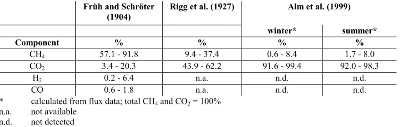
(cf. Davidson, 1991). An analysis of gases emitted from peatlands is given in Table 2-4.
8 “Wetlands”, a more general term, which includes also mires with less than 30 cm peat thickness (Lappalainen,
1997) and other waterlogged soils as for example floodplains, coastal lagoons, mangroves, swamps, rice paddies, represent the major source of methane to the atmosphere. This is even the case, when both natural and anthropogenic sources are considered (e.g. Hein et al., 1997; Houwelling et al., 1999; cf. Fig. 2-4).
Table 2-4: Composition of “marsh gas” for different European and North American mires. The high discrepancy
between early and recent study may not only be attributed to the different mires investigated but also to the technical development of chemical analysis.
Früh and Schröter
(1904) Rigg et al. (1927) Alm et al. (1999)
winter* summer* Component % % % % CH4 57.1 - 91.8 9.4 - 37.4 0.6 - 8.4 1.7 - 8.0 CO2 3.4 - 20.3 43.9 - 62.2 91.6 - 99.4 92.0 - 98.3 H2 0.2 - 6.4 n.a. n.d. n.d. CO 0.6 - 1.8 n.a. n.d. n.d. * calculated from flux data; total CH4 and CO2 = 100%
n.a. not available n.d. not detected
At present, northern hemisphere peatlands indirectly have a negative radiative forcing effect, i.e. they ‘cool the atmosphere’, because CO2 uptake by plant growth and organic matter
accumulation compensates for the warming effect of peatland CH4 emissions (Martikainen,
1997). The level of the water table in the peatland is of outstanding importance for the actual greenhouse gas emissions from mires and, in turn, for the potential feedback of peatlands to global and regional climatic change. A possible lowering of the water level as a consequence of reduced rainfall or higher evapotranspiration, for instance, would, within a few months and years already, increase the CO2 and N2O emissions (Kettunen et al., 1996; Nykanen et al.,
1998), but reduce the CH4 release (Moore and Knowles, 1989, 1990; Freeman et al., 1993;
Martikainen et al., 1993). According to Nykanen et al. (1997), lowering the water table in a boreal mire by only 1 cm, would increase the CO2-C release by 10 g*m-2*y-1. A fundamental,
yet very recent object of research is the question, how peatland gas production will change in response to global warming. Incubation experiments carried out so far show for most peatland types increasing methane (and CO2) production at higher temperatures (Updegraff et al.,
1998).
2.7 Methane emissions from peatlands
Recent estimates for the global methane release from peatlands to the atmosphere range from 145 Tg/a (Houwelling et al., 1999) to 237 Tg/a (Hein et al., 1997) and make up for more than 80 % of all natural and about 25 to 40 % of the total, i.e. natural and anthropogenic, emissions (cf. Fig. 2-4; IPCC, 2001). The total amount of methane emitted from northern hemisphere peatlands is estimated at 35 or 38 Tg (1012 g) per year (Fung et al., 1991; Bartlett and Harriss, 1993, respectively). Northern peatlands contribute hence to about one third to the total natural wetland source.
Most of the pioneering studies (e.g. Panikov et al., 1993) concerned with methane emission from peatlands try to explain the methane emission only in respect to the bulk area of the peat. There is now an increasing number of very specific investigations, for example concerned with the seasonal methane fluxes: According to Alm et al. (1999), for instance, summer fluxes of methane from the bog surface may be up to 15 times higher than winter fluxes. Other studies are concerned with the contribution of single peatland plants to CH4 emissions (e.g.
inorganic ions (e.g. Dise and Verry, 2001) on peatland methane production. Methane emissions may vary very much from peatland to peatland. The reported fluxes range from <1 to 3200 mg CH4 m-2*d-1 (Shotyk, 1989b; Bubier et al., 1993; Glenn et al., 1993; Roulet et al.,
1994; Shannon and White, 1994; Martikainen et al., 1995; Alm et al., 1999). The actual methane production in the peat is however higher, as important quantities of methane are oxidised in the acrotelm (e.g. Sundh et al., 1995) or in plant stems (Frenzel and Rudolph, 1998) and hence not emitted into the atmosphere. During the last years, scientists were able to isolate a range of acidophilic methane-oxidising bacteria from northern peatlands (Dedysh et al., 1998). Oxidation rates may range from ca. 30 to 50 % of the methane produced (Holgate 1990; Frenzel and Karofeld, 2000). In some rare cases and depending very much on the watertable, up to 100 % and more of the methane are oxidised. Methane concentrations in the uppermost part of the acrotelm may then fall below atmospheric levels (ca. 2 ppm) leading to CH4 flow from the atmosphere into the peat (Martikainen et al., 1995; Roulet and Moore,
1995).
2.8 How does methane form in peatlands?
Fig. 2-5: Successive
reductions during the aerobic-anaerobic transition. After aerobic respiration (1) has exhausted available oxygen, anaerobic denitrifying bacteria (2), facultative and iron-reducing bacteria (3) reduce nitrate and iron, with a concomitant lowering of the redox potential of the medium. Fermentation reactions can take place, giving rise to metabolites (alcohols, organic acids) that can be utilised by obligate anaerobic bacteria. The sulphate and sulfur-reducers occur first (4). The ‘climax’ stage of methanogenic syntrophy (5 and 6) produces marsh gas, a mixture of methane and carbon dioxide. It is produced only at the end of the process, if oxidisable substrates are still available (according to Gobat et al., 1998).
- CO2 reduction and acetate splitting -
While the actual emission calculations are widely acknowledged, the occurrence and relative importance of biochemical pathways that lead to methane formation (“methanogenesis”) in wetlands are still vividly debated (e.g. Hornibrook et al., 1997; Waldron et al., 1998).
Methane is an end product of anaerobic decomposition processes in peatlands. Methanogenesis only becomes a competitive microbial metabolic process in the absence of oxidation processes with molecular oxygen and other potential electron acceptors (e.g. NO3-;
Fe3+; SO42-), which yield more energy (“reduction séquentielle”, Gobat et al., 1998; cf. Fig.
2-5).
Two major methanogenic pathways are distinguished: CO2 reduction and methylotrophism. CO2 reduction is a microbial metabolic process, where CO2 (or HCO3-) is converted into
methane. The necessary electrons predominantly derive from oxidation of H2. Methylotrophic
bacteria by contrast catabolise organic compounds that contain methyl groups (e.g. methanol, ethanol, dimethyl sulphide, methylated amines). The methyl groups are reduced to CH4 using
electrons from oxidation of other methyl groups or from hydrogen. Acetoclastic
methanogenesis is a special case of methylotrophism, as the electrons used for reduction of
the acetate’s methyl group derive from its carboxyl group, which is oxidised to CO2 (Boone et
al., 1993). The study of concentration patterns and the carbon stable isotope composition of CH4 (and co-existing CO2) is not only a powerful tool to identify and to evaluate the various
sources of methane in the environment (cf. Cicerone and Oremland, 1988), but also to characterise the microbial methanogenic processes (e.g. Whiticar et al., 1986). This is the major objective of this thesis.
The following questions are therefore addressed:
- What are the concentrations of acetate and other volatile fatty acids (VFA) such as formate
and propionate in the catotelm of the Etang de la Gruère Bog? How and why are these concentrations changing during the seasons? Are these changes reflected in the methane concentration patterns? Confer chapter 6.1.
- Given the isotopic evidence, is there a significant shift in the methanogenic pathway with
time or with depth? To our knowledge, this is the first investigation of peat methanogenic processes up to 6 m below ground surface. How do the results correlate to studies at other bogs and what are the possible reasons for the discrepancies? Confer chapter 6.2.
- What are agreements and disagreements, when the observed concentration patterns and
3 THE STUDY SITES
3.1 Etang de la Gruère (EGr)
The principal site of field research for this study is the Etang de la Gruère peat bog (EGr) in NW Switzerland. It has been chosen for the following reasons:
- Availability of background information: The EGr field site had already been very well
studied and considerable information on biological, hydrological and geochemical aspects are available. In the following, some examples of earlier research work at EGr with focus on different fields of research are given: Paleobotany and palynology (Joray, 1942), conservation (Büttigkofer, 1942), peatland ecology (Feldmeyer-Christe, 1990), peat pore water geochemistry (e.g. Steinmann, 1995; Steinmann and Shotyk, 1997a, Steinmann et al., 1998) and peat chemistry (Steinmann and Shotyk, 1997b), age dating of peat and atmospheric lead deposition (Shotyk et al., 1998; Shotyk et al., 2001), peat pore water carbon stable isotopes (Steinmann et al., 2000), peat pore water hydrology (McKenzie et al., 2002), and lithogenic trace metals (Shotyk et al., 2001). In addition, F. Roos from Bern University currently carries out a research project about heavy metal, especially Hg, deposition in the peat record (scientific direction by W. Shotyk from Heidelberg University), which allowed the use of similar field instrumentation and the exchange of data, samples, and information.
- Thickness of the peat layer: Since it has been the aim to study also the pore water
chemistry of the deeper acrotelm, a bog with sufficiently thick peat was indispensable. At the EGr study site, the peat thickness exceeds 6 m. This thickness of peat deposition exceeds that of most boreal bogs (3 - 4 m; Maltby and Proctor, 1997). In addition, the selected site is characteristic for the EGr Bog as well as for other boreal peat bogs with respect to surface vegetation and peat matrix.
- Location and accessibility: The EGr can easily be reached by car. The distance from
Neuchâtel and hence from the laboratory facilities is just about 50 km. This proved to be particularly important for determining instable organic acid concentrations as quickly as possible.
In general understanding, the term “Etang de la Gruère” denotes by far more the artificial lake (fr. étang = pond, small lake) than the peat complex around it (Fig. 3-1). Therefore, the usage of “Etang de la Gruère Bog” is a viable alternative to address exclusively the raised mire, i.e. not the lake nor the relatively small swamp, fen, and transitional zones being present at the Etang de la Gruère as well. For simplification,
however, the mere topographic name (or “EGr” in abbreviation) will also be used in this study to designate the bog.
Fig. 3-1: Photograph
showing a part of the Etang de la Gruère The Etang de la Gruère has been included in
several Swiss Federal Inventories of Mires of National Importance: Inventory of Raised and Transitional Mires, 1991 (Mire no. 2; cf. Grünig et al., 1984); Inventory of Fen-Mires, 1994 (Mire no. 1312; cf. OFEP, 2000); Inventory of Particularly Beautiful Mires, 1996 (Mire no. 7; cf. OFEP 2000).
While in older literature (especially in documents written between the 16th and the 19th century; cf. Mulhauser, 1996) “Etang de la Gruère” is mostly written with a “y” (“Gruyère”), this soft-sounding, unaspirated letter often drops out in more recent writing to avoid confusion with the Gruyère Region in the Swiss Canton of Fribourg.
Etymologically, two different explanations are given for the name of the site: “Gruère” (or “Gruyère”) has been the historic term for a woodland domain under the patronage of a local lordship (Mulhauser, 1996). The second explanation (Wermeille, 1998) relates “Gruère” to the German word “Grütze” (groats), a rather general name for several products ground in a mill. The Etang de la Gruère Lake has first been dammed in middle of the 17th century to supply waterpower for a mill, which was in use for more than 300 years (from about 1650 to 1952; cf. Mulhauser, 1996).
3.1.1 Physiographical setting
The Federal-Reserve EGr lies in the Franches Montagnes, which is a karstic plateau within the Folded Jura in NW Switzerland (Fig. 3-2). The EGr lake and peat bog is located 4 km SE of Saignelégier around 100 m N of the Road Saignelégier-Tramelan (Fig. 3-3).
Fig. 3-2: Location of the
Etang de la Gruère in Northwest Switzerland’s Jura Mountains.
500 m
Saignelégier
Tramelan
sampling site on peninsula Fig. 3-3: Swiss topographic map 50 (scale 1 : 50,000): Detail of the Etang de la Gruère region.The bog covers a total area of 22.5 ha on a remarkably domed peninsula and the lake margins (Fig. 3-4). The elevation of the bog is approximately 1000 m asl. (994 to 1002 m). The surrounding hillocks are 20 to 50 m higher (cf. Fig. 3-3). The elevation above sea level of the Franches Montagnes ranges between ca. 500 m (banks of the river Doubs) and ca. 1100 m (“Sur le Peu”) with wide peneplain sections at about 1000 m asl.. The plateau is open towards N and W, whereas towards SE, it is flanked by two consecutive mountain chains, the Montagne du Droit (1263 m) and the Chasseral (1607 m).
Fig. 3-4: Vertical cross-section of the Etang
de la Gruère peat bog. The arrows indicate the assumed water flow regime (cf. chapter 5.2.5). The “S” marks the location of the main sampling site. The shaded area in the middle of the peninsula refers to a zone with increased peat decomposition (after
Steinmann and Shotyk, 1997a).
Most of the EGr Bog is covered by a loose spruce and pine tree forest with Pinus unicata prevailing. The sampling site lies in an open part (“Oeil de l’Etang de la Gruère”) almost in the middle of the domed peninsula (cf. Fig. 3-3). The open part shows faint development of hummocks and hollows. Its surface vegetation is dominated by Sphagnum magellanicum in the hollows and Sphagnum rubellum on the hummocks (Feldmeyer-Christe, 1990).
3.1.2 Geological setting
The EGr peat complex formed in a local depression, where organic matter has accumulated since the end of the Pleistocene and throughout the entire Holocene. Radiocarbon age dating indicates first peat formation at ca. 12,370 14C years (about 14,500 years BP, Shotyk et al., 1998). The substrate is clay derived from Oxfordian (lowest Upper Jurassic) clays and marls. As pollen-based dating of the clays did not yield ages older than 12,000 years (Joray, 1942), reworking of the clays and marls is assumed (Steinmann, 1995). Reworking of clays and marls may occur as a result of the movements of local ice-sheets or by flowing water over a frozen karstic ground during and at the end of times of glaciation. The Oxfordian clays occur in the core of the “Les Bois-Paturatte” anticline and are confined by more resistant “Argovian” (lower Upper Jurassic, yet, strictly speaking not a chronostratigraphic unit) marly limestones (Forkert, 1932). The underlying “Dalle nacrée” (massive slab-shaped limestone) is exposed in a culmination of the anticline (Gros Bois Derrière) about one kilometre to the WNW (Steinmann, 1995).
The local depression in which the EGr is situated has an ellipsoidal shape and a length of ca. 900 m, a width of 200 - 300 m, and an average depth of about 30 m (cf. Fig. 3-3). Its long axis strikes almost 60° (i.e. ENE) and thus parallels the major folding of the Jura Mountains. Secondary overprinting by local glaciation during the last ice age, however, cannot be excluded. Yet so far, no direct evidence for glaciation (e.g. local, kar-like glacier deposits) has been found (Mulhauser, 1996). There is, however, indirect evidence that peat formation followed a period of glaciation at the EGr: Basal clays still contain carbonate and hence had probably not been subject to intense weathering (Joray, 1942) as would be the case for substratum marls exposed to moderately warm climate. The age dating indicates that the accumulation of organic matter could have started directly upon melting of the glacier ice and formation of the periglacial, non-artificial, EGr lake.
3.1.3 Climate
The EGr region is characterised by a humid, temperate zone mountain climate. Long-term climatological data (Fig. 3-5) refer to the international standardised 30 years’ average (MeteoSwiss Costumer Service, Zürich) of values measured for the time period from 1961 to 1990 at Saignelégier (ca. 4 km WNW’ of EGr - precipitation) and La Chaux-de-Fonds (ca. 20 km SW’ of EGr - temperature) meteorological stations (MeteoSwiss Costumer Service, Zürich): Temperature variation (annual mean 5.8 °C) shows continental influence, with a daily mean temperature of 15 °C in the warmest (July) and of -5 °C in the coldest month (January). Precipitation, however, is high (annual mean 1511 mm) due to the elevation above sea level and the Franche Montagne’s exposition in the luff of predominant northwesterly winds. Typically, a snow-cover is present for a period of 80 to 120 days per year.
Fig. 3-5: Mean monthly
precipitation and temperature for the time period from 1961 to 1990 measured at the MeteoSwiss meteorological stations (precipitation: Saignelégier; temperature: La Chaux-de-Fonds) in the Franches Montagnes region. For the Saignelégier
meteorological station, which is closer to the field site (cf. text), the 30 year temperature average was not available (data from MeteoSwiss Costumer Service, Zürich).
3.1.4 Peat characteristics
An account on the history of peat deposition at the EGr and the biological diversity of the different peat-forming plants is given by Steinmann (1995).
Fig. 3-6 schematically shows the peat stratigraphy at the sampling site along with the pH profile and ash contents. Low pH values of 4.5 and below near the bog’s surface for both, the pore waters and the solid matrix are typical for raised ombrogenic peat lands. Similar values are, for example, reported for a large number of peat bogs in North America, northern Europe (Shotyk, 1988), and Siberia (Inisheva et al., 2000). At the Etang de la Gruère, pore water pH values increase steadily with depth. After a relative gentle increase to about 3.5 m (ca. pH 5.5) below ground surface, the pH increase is more pronounced in the lower catotelm and the bog pore water’s pH gets close to neutral values at about 6 m (ca. pH 6.5) below ground surface. Steinmann (1995), observed the same trend, yet with even slightly lower pH values in the upper catotelm (above ca. 3 m depth). The strong pH increase in the lower bog can be explained by mixing of pore waters derived from the substratum (carbonate minerals in marly
clays and marls - cf. chapter 3.1.2). In the study presented here, comparable relative pH patterns have been observed for all measurement series (cf. chapter 5.2.1), absolute pH values for the pore water in the lower catotelm were however consistently lower than those reported by Steinmann (1995). A significant seasonal variation of the pH at EGr was not observed (chapter 5.2.1). The pH values for peat suspended in deionised water were lower than those for the pore water. The difference is particularly large for the lower catotelm what again highlights the influence of the substratum on the peat pore water.
Fig. 3-6: Peat stratigraphy at
the coring site (EGr) along with the pH profile and the ash contents. Filled stars in the pH profile refer to pH values of pore waters, open circles refer to pH values of peat suspended in deionised water. S:
Sphagnum peat, Er: Eriophorum peat, C: Carex peat, NL: remains of shrubby plants. The H-values (e.g. “H8”) refer to the “Von Post scale” of humification (from Steinmann, 1995).
The ash content in peat is a measure for the share of the peat’s mineral (i.e. the non-organic matter) content. According to Steinmann (1995), the ash content at EGr generally increases with depth and reaches an average value of almost 9 wt-% at the base of the bog reflecting the early bog forming conditions. On the other hand, this means an organic matter content of over 90 wt-% and even more than 95 wt-% in the first ca. 4 m of the bog. There are in the EGr bog distinct (cm scale) layers with a considerably higher mineral content of up to 30 wt-% (P. Steinmann - pers. comm.).
The degree of humification (cf. Fig. 3-6) is conveniently expressed by descriptive classification according to the “Von Post scale” (Von Post and Granlund, 1925). Changes in peat land vegetation, in climate and / or the accumulation rate of organic matter influence humification. At EGr, a zone of more decomposed peat (H8, according to the Von Post humification scale) is situated between 130 and 370 cm (Steinmann, 1995). Accordingly, the vertical hydraulic conductivity of this zone is much lower than above and below (10-4 cm/s; McKenzie et al., 2002; cf. chapter 5.2.5). The possible implications of the peat structure for the pore water chemistry and turnover of chemical species are discussed in chapters 6.1 and 6.4.4.
3.2 Other field sites
Work on the two further field sites, the “Tourbière de la Chaux-des-Breuleux” in Switzerland and the “Vasjugan Bog” in Russia, is the result of cooperation with scientists from other institutions working on related issues, i.e. the Microbiology Laboratory of the Biological Institute at Neuchâtel University and the Tomsk-based Russian Academy of Agricultural Sciences’ Institute of Peat, respectively.
The Tourbière de la Chaux-des-Breuleux is situated in the Franches Montagne Region about 3 km south of EGr in Switzerland’s northwest Jura Mountains. The average elevation of the bog above sea level is about 990 m. The other physiographical and climatological aspects of that site are also very similar to EGr. For a detailed description of the Tourbière de la Chaux-des-Breuleux, cf. Maeder (2000).
The Vasjugan Bog (Fig. 3-7) is situated in the southern part of West Siberia between the cities of Omsk, Novosibirsk, and Tomsk. It is the world’s largest coherent bog covering 50,000 square kilometres of lowlands between the Ob and Irtysh Rivers. It has an average depth of 3 to 4 meters and contains ca. 19 * 109 t of peat, i.e. 16 % of the total peat reserves in West Siberia (Inisheva et al., 2000). Scientific research conducted with respect to the Vasjugan Bog has mainly concentrated on peat amelioration and potential agricultural use. An enormous effort has been made to regionally classify and characterise the different mire types. A detailed peat stratigraphy is
therefore available for various representative sites.
The Vasjugan Bog’s elevation above sea level ranges from ca. 50 to 95 m. The climate is strongly continental with short, warm summers and long, extremely cold winters. The average annual precipitation varies from 700 to 850 mm. For a detailed description of the Vasjugan Bog, cf. Inisheva et al. (2000).
Fig. 3-7: Aerial
photograph showing an oligotrophic province of the Great Vasjugan Bog, West Siberia (by W. Bleuten in IPS, 2002).
4 METHODS
4.1 Sampling of bog pore waters
Pore water samples were obtained in situ with plexiglass diffusion chambers ("peepers"; cf. Steinmann and Shotyk, 1996), which allow diffusion between the bog pore water and the liquid in the chamber. Figs. 4-1a and 4-1b show the two different types of peepers used for pore water sampling near the surface (Type A) and in the deeper bog (Type B).
top-view side-view Fig. 4-1a (right):
Illustration of peeper Type A.
Peeper Type A consists of a 2 x 15 x 70 cm thick plexiglass body (B) with chambers (C). Membrane filters (M) are held in place by 0.5 cm thick plexiglass lids (L) and nylon screws (S) (from Steinmann and Shotyk, 1996).
Fig. 4-1b (left): Illustration of
peeper Type B.
Peeper Type B is a single chamber (C) cut from a 15 cm long plexiglass bar (4 x 4 cm). Membrane filters (M) are held in place by plexiglass lids (L) fixed with cable binders (B). The polypropylene connecting tubes (T) are sealed against the interior (X) to prevent the introduction of O2 or
near-surface waters, when the peepers are installed (from Steinmann and Shotyk, 1996).
M
side-view top-view assembled
The peepers had been designed for an earlier fieldwork at EGr. A. Steinmann from Schötz (Switzerland) and technicians of the University of Bern (Switzerland) manufactured the peeper sets. They were used by P. Steinmann for his PhD project Steinmann (1995) at the same site and left to the author for this study. Fig. 4-2 shows schematically, how the two peeper types were installed at the EGr field site.
Fig. 4-2: Schematic
illustration of the peeper configuration in the EGr Bog. Peeper Type A was installed as a single piece near the surface, whereas Type B peepers were connected to each other by tubes or special connectors and could be hence also be used for pore water sampling in the deep catotelm. Usually, either 11 or 12 peepers of Type B were installed for each sample series.
Shallow pore water profiles were sampled with a short, flat (2 cm thick) plexiglass body containing 20 parallel chambers (Type A, cf. Fig. 4-1a). The volume of the chambers is approximately 30 ml. Both sides of the peeper are covered with a 0.2 mm polysulfone filter membrane, which is available in rolls (Gelman, U.S.A). A 0.5 mm mesh polypropylene screen (Lanz-Anliker, Switzerland) protects the membrane against damage by wood or roots. Both the membrane and the screen are held in place by lids with a frame, which fits the chambers. The lids are fixed to the peeper chambers by nylon screws. As the total surface of the membranes covering each chamber on both sides is 30 cm2, approximately one square centimetre of membrane per millilitre of sample volume is available for ion and molecule
exchange with the pore water. Peeper A has a total length of 75 cm. The length of the chamber assembly, however, is only 50 cm. Due to the small distance between each chamber milled into the plexiglass body, the depth resolution of this sampling technique is relatively high (ca. 2 cm). The sampling range of Type A peeper is variable and depends on the depth of insertion into the ground. In the study presented here, the sampling range was between 23 and 73 cm.
The deeper bog pore water profiles were sampled using single diffusion chambers (Type B peepers). The chambers were milled from a plexiglass bar with a quadratic 4 x 4 cm cross section (Fig. 4-1b). The chamber volume is also approximately 30 ml. As the total surface of membrane covering the chamber on both sides is ca. 25 cm2, 0.8 cm2 of membrane per millilitre of sample volume are available for exchange with the pore water. Alike Type A, the chambers of peeper Type B are covered by a filter membrane (0.2 µm polysulfone membrane; produced by Schleicher & Schuell, Germany), a polypropylene screen (mesh size 0.5 mm; Lanz-Anliker, Switzerland) to prevent damage of the membrane and a plexiglass lid. Nylon cable binders are used to attach the lids at the two sides of each chamber.
On the field site, the single Type B diffusion chambers were linked to each other with polypropylene tubes (ca. 50 cm long) and connectors (variable length from 5 to 14 cm). Nylon screws were used for fixing the tubes or connectors to the peepers (cf. Fig. 4-1b). The depth resolution of this sampling technique varied between 14 and 60 cm depending on the configuration of chambers, tubes and connectors. Since up to 12 diffusion chambers could be linked at a time, the depth range of the Type B peepers was from ca. 50 to 590 cm below ground surface. Two such sets of Type B peepers (with 12 and 11 diffusion chambers, respectively) were available and were alternately installed in the bog.
Prior to the first use in the field, all plexiglass parts had been leached in 10 % nitric acid and then extensively washed with deionised water. Before each field campaign, all plexiglass parts were leached another time in 10 % nitric acid and then extensively rinsed with deionised water. At the end of each sampling campaign the peepers and lids were thoroughly washed, first with tap water, then with deionised water, before being stored in sealed polyethylene boxes in the laboratory.
In the morning before each sampling campaign, all components used were carefully rinsed with deionised water. The filling procedure was different for the two peeper types and was performed in the laboratory in Neuchâtel: Peeper Type A was first put, the open side up, in a plexiglass box constructed for this purpose. Deionised and degassed water (electrical resistivity >17 Ω/m) was poured into the box, until the peeper chambers were entirely filled. Then, the membrane, screen and lid were mounted on the upper side. Finally, the box was completely filled with deionised and degassed water and sealed for transport.
As for peeper Type B, the diffusion chambers were first provisionally closed on the lower side by pressing a moistened membrane (plus screen and lid) gently against the chamber. Subsequently, the chamber was filled with deionised and degassed water and then carefully covered on the upper side with the membrane to avoid trapping air bubbles in the chamber. Afterwards, the lids were fixed on both sides with cable binders. For transport, the so-prepared peepers were stored in deionised (resistivity >17 Ω/m) and degassed water in a sealed polyethylene container. In order to degas (deaerate) the deionised water nitrogen (99.995 vol-%) was injected for 30 to 40 minutes into a slim receptacle containing deionised water, allowing the bubbles to ascent in a long water column. In particular, this was necessary to remove the potentially remaining dissolved oxygen from the peeper liquid.
Upon arrival on the field site (and usually after sampling and removal of the previous set of peepers), the new peepers were installed. For peeper Type A, a rectangular (ca. 4 x 20 cm) and about 80 cm deep hole was cut into the peat using different knifes and an axe. The peeper set was then installed as shown in Fig. 4-2 and covered with the original sod.
For peeper Type B, no new hole was necessary, as a pre-existent core hole drilled for an earlier research project (cf. Steinmann, 1995) could be used. On the field site, the diffusion chambers were linked to each other using the polyethylene tubes and connectors shown in Fig. 4-2. Set up of the peeper configuration and installation into the ground was done progressively and in vertical position by screwing each time the appropriate part of the configuration to those already installed in the ground hole (Fig. 4-3). The tubes were plugged with silicone-clad rubber stoppers to
prevent introduction of air (O2) or larger
volumes of near surface waters at depth. In addition, a certain degree of buoyancy could hence be maintained. The buoyancy effect slowed the drowning of the assembly down and thus reduced the risk of component loss and of the hole being blocked. Upon completion of the set up, the hole was covered with the original sod.
The peepers usually remained for five to seven weeks in the bog, what is largely sufficient for the chamber liquid to equilibrate with the pore water in the peat
(Steinmann and Shotyk, 1996). The peepers were removed from the peat using a small chain, which was drawn through a hole at the top of the peeper (Type A) or at the top of the uppermost tube (Type B). The peepers were removed from the bog at once (Type A) or, in case of Type B, by progressively, one by one, dismembering the diffusion chambers from the assembly. As the hole narrowed considerably, even within a relatively short time interval of few weeks, due to lateral pressure, pulling out of the peepers sometimes proved to be outright difficult. This was particularly the case for the long, 12 diffusion chambers comprising configuration of peeper Type B.
Fig. 4-3: Installation
of a new set of Type B peepers. Field
assistant: M. Gurk (photograph by U. Helg).
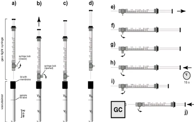
Latex gloves (rinsed with deionised water) were used, whenever the diffusion chambers had to be touched for filling, sealing, fixation and sampling (Fig. 4-4). For sampling, new, sterilised, single use material including standard syringes, needles and vacutainers was used (cf. Fig. 4-4). The needles had a wide orifice to reduce low pressure and potential degassing, when the samples were taken. Vacutainers are evacuated and sealed glass-tubes, widely used for blood sampling. The vacutainers chosen for pore water sampling had a guaranteed evacuated volume of 7 ml (total volume 8.2 ml) and a silicone-clad poly-buthylene rubber seal.
Fig. 4-4: Sampling of a peeper Type B. The
liquid in the peeper chamber is transferred into a vacutainer using a standard plastic syringe (photograph by U. Helg).