HAL Id: hal-00804747
https://hal.inria.fr/hal-00804747
Submitted on 26 Mar 2013
HAL is a multi-disciplinary open access
archive for the deposit and dissemination of
sci-entific research documents, whether they are
pub-lished or not. The documents may come from
teaching and research institutions in France or
abroad, or from public or private research centers.
L’archive ouverte pluridisciplinaire HAL, est
destinée au dépôt et à la diffusion de documents
scientifiques de niveau recherche, publiés ou non,
émanant des établissements d’enseignement et de
recherche français ou étrangers, des laboratoires
publics ou privés.
Failure Analysis and Modeling in Large Multi-Site
Infrastructures
Minh Tran Ngoc, Guillaume Pierre
To cite this version:
Minh Tran Ngoc, Guillaume Pierre. Failure Analysis and Modeling in Large Multi-Site Infrastructures.
13th International IFIP Conference on Distributed Applications and Interoperable Systems, IFIP, Jun
2013, Florence, Italy. �hal-00804747�
Multi-Site Infrastructures
Tran Ngoc Minh and Guillaume Pierre
IRISA / University of Rennes 1, France {minhtn,guillaume.pierre}@irisa.fr
Abstract. Every large multi-site infrastructure such as Grids and Clouds must implement fault-tolerance mechanisms and smart schedulers to en-able continuous operation even when resource failures occur. Evaluating the efficiency of such mechanisms and schedulers requires representative failure models that are able to capture realistic properties of real world failure data. This paper shows that failures in multi-site infrastructures are far from being randomly distributed. We propose a failure model that captures features observed in real failure traces.
1
Introduction
Large computing infrastructures such as Grids and Clouds have become indis-pensable to provide the computing industry with high-quality resources on de-mand. However, failures of computing resources create an important challenge that these infrastructures must address. Failures cause a reduction of the total system capacity, and they also negatively impact the reliability of applications making use of the resources. Understanding failures from a statistical point of view is therefore essential to design efficient mechanisms such as checkpointing and scheduling in Grids and Clouds.
This paper presents a comprehensive analysis of failure traces from five large site infrastructures [10]. We focus on simultaneity, dependence and multi-plication features. Simultaneity measures the extent to which multiple failures or multiple recoveries happen at the same time. Dependence means that times between failures have short- and long-term autocorrelations. Finally, multiplica-tion captures the fact the times between failures are not smoothly distributed but rather occur at multiples of specific durations. Similar features were not present in previous studies of clusters, peer-to-peers and web/dns servers. We therefore believe that they are characteristic of large multi-site systems. This analysis enables us to model failures and generate realistic synthetic failure sce-narios that can be used for further studies of fault-tolerance mechanisms. The advantage of a failure model is that it enables us to tune parameters as we wish, which is not possible when replaying a trace.
This analysis is based on five traces of node-level failures from the Failure Trace Archive [10]. These traces, described in Table 1, can be considered as representative of both Grid and Cloud infrastructures. For example, GRID’5000
which is currently used to serve Cloud users is a good representative of low-level Cloud infrastructures. However, since these traces were collected when serving Grid jobs, obviously virtualization is another source of failures in Clouds that we do not consider.
This paper is organized as follows. Sections 2, 3 and 4 respectively analyse the simultaneity, dependence and multiplication properties in failure traces. Sec-tion 5 proposes a failure model that SecSec-tion 6 validates with real world data. Finally, Section 7 discusses related work and Section 8 concludes the paper.
Table 1. Details of failure traces used in our study.
ID System Nodes Period, Year Res.1 #(Un)availability Events
MSI1 CONDOR-CAE 686 35 days, 2006 300 7,899 MSI2 CONDOR-CS 725 35 days, 2006 300 4,543 MSI3 CONDOR-GLOW 715 35 days, 2006 300 1,001 MSI4 TERAGRID 1,001 8 months, 2006-2007 300 1,999 MSI5 GRID’5000 1,288 11 months, 2006 5 419,808
2
Simultaneity of Failures and Recoveries
Let T be a set of N ordered failures: T = {Fi|i = 1 . . . N and Fi≤ Fj if i < j},
where Fi denotes the time when a failure i occurs. Each failure i is associated
with an unavailability interval Ui, which refers to the continuous period of a
service outage due to the failure, and the time Ri = Fi + Ui indicates the
recovery time of the failure. For a group of failures T0 that is a subset of T , we
consider a failure i as a simultaneous failure (SF) if there exists in T0any failure
j 6= i such that j and i happen at the same time, otherwise we call i a single failure. Similarly, we also consider i as possessing a simultaneous recovery (SR)
if there exists in T0any failure k 6= i such that k and i recover at the same time,
otherwise i possesses a single recovery.
Assigning T0 as a whole failure trace, we calculate the fractions of SFs and
SRs in real multi-site systems, which are shown in the first and second rows of Table 2. As we can see, simultaneous failures and recoveries are dominant in all cases. We do a further analysis to check how many simultaneous failures possess SRs. This is done by determining all groups of SFs, i.e. all failures that occur at the same time are gathered into one group, and calculating the number of SRs for each group. We then average and show the result in the third row of Table 2. We conclude that most of the simultaneous failures recover simultaneously.
Considering each trace separately, failures of MSI1 and MSI2 almost occur and reoperate concurrently, so it is not surprising when most of the simultaneous 1 Res. is the trace resolution. For instance, a node failure at time t with resolution 5
Table 2. Fractions of SFs (R1) and SRs (R2) in real systems, calculated for the whole trace. The third row (R3) shows fractions of SRs, calculated for groups of SFs.
MSI1 MSI2 MSI3 MSI4 MSI5 R1 97% 93% 75% 73% 95% R2 98% 97% 81% 75% 95% R3 97% 98% 94% 93% 69%
recoveries belong to SFs. But this does not apply for MSI5, where only 69% resources with SF become available simultaneously despite of a large number of SFs and SRs (95%). This is due to failures that occur but do not recover at the same time with some failures, instead they recover concurrently with other failures. In contrast with MSI5, MSI3 and MSI4 only exhibit around 70%-80% SFs and SRs but a large number of SRs are from SFs. One can think of the resolution of the traces as the reason that causes SFs and SRs. However, we argue that the resolution is not necessarily a source of the simultaneity feature since the resolution is relatively small and cannot cause such a large number of SFs and SRs. A more plausible reason that causes a group of nodes to fail at the same time is that the nodes share a certain device/software whose failure can disable the nodes. For example, the failure of a network switch will isolate all nodes connected to it. Its recovery will obviously lead to the concurrent availability of the nodes.
We believe that the simultaneity feature is common in data-center-based systems. We therefore argue that fault-tolerant mechanisms or failuaware re-source provisioning strategies should be designed not only to tolerate single node failures, but also massive simultaneous failures of part of the infrastructure.
3
Dependence Structure of Failures
We now deal with a set of times between failures {Ii}, whose definition is based
on the set of ordered failures T = {Fi} in Section 2. We determine a time between
failures (TBF) as Ii= Fi− Fi−1and hence it is easy to represent {Fi} by {Ii} or
convert {Ii} to {Fi}. This section examines the dependence structure of {Ii}2.
The term “dependence” of a stochastic process means that successive samples of the process are not independent of each other, instead they are correlated. A stochastic process can exhibit either short or long range dependence (SRD/LRD) as shown by its autocorrelation function (ACF). A process is called SRD if its ACF decays exponentially fast and is called LRD if the ACF has a much slower decay such as a power law [3]. Alternatively, the Hurst parameter H [7], which takes values from 0.5 to 1, can be used to quantitatively examine the degree of dependence of a stochastic process. A value of 0.5 suggests that the process is either independent [1] or SRD [11]. If H > 0.5, the process is considered as LRD, where the closer H is to 1, the greater the degree of LRD.
2
MSI1 MSI2 MSI3 MSI4 MSI5 0.4 0.5 0.6 0.7 0.8 0.9 1 System Hurst estimate 0 3 6 9 12 15 18 −0.2 0 0.2 0.4 0.6 0.8 1 Lag ACF MSI1 0 3 6 9 12 15 18 −0.2 0 0.2 0.4 0.6 0.8 1 Lag ACF MSI2 0 3 6 9 12 15 18 −0.2 0 0.2 0.4 0.6 0.8 1 Lag ACF MSI3 0 3 6 9 12 15 18 −0.2 0 0.2 0.4 0.6 0.8 1 Lag ACF MSI4 0 3 6 9 12 15 18 −0.2 0 0.2 0.4 0.6 0.8 1 Lag ACF MSI5
Fig. 1. Hurst parameter and autocorrelation functions of TBFs in real traces.
Figure 1 shows the dependence feature. To quantitatively measure how TBFs are autocorrelated, we estimate the Hurst parameter of real TBF processes. The estimation is done with the SELFIS tool [9]. As there are several available heuris-tic estimators that each has its own bias and may produce a different estimated result, we chose five estimators (Aggregate Variance, R/S Statistic, Periodogram, Abry-Veitch and Whittle) and computed the mean and the standard deviation of their estimates. For all cases real TBFs are indeed LRD because all Hurst estimates are larger than 0.5. The most noticable point focuses on MSI2, MSI3 and MSI4, which result in H around 0.7 to 0.8. It shows that the TBFs of these traces are largely autocorrelated. This is confirmed by observing their ACFs in Figure 1, which decay slowly and determine their LRD feature. The LRD of MSI1 and MSI5 are not very strong since their estimated Hurst parameters are larger but not very far from 0.5. In particular, the ACF of MSI1 decays though not exponentially but quickly to 0, thus one can also consider it as SRD or in our case, we call it as exhibiting weak LRD.
It is important to capture the LRD feature in modeling because it may signif-icantly decrease the computing power of a system by the consecutive occurrence of resource failures. In particular, if simultaneous failures happen with LRD, a system will become unstable and it is hard to guarantee quality-of-service re-quirements. Fault-tolerant algorithms should therefore be designed for correlated failures to increase the reliability.
4
Multiplication Feature of Failures
An interesting feature of failure traces is the distribution of times between fail-ures. However, we have seen that the vast majority of failures are simultaneous. This would result in several TBFs with value 0 as shown in Table 3. The oc-curence of a large number of zeroes in a TBF process makes it difficult to fit TBFs to well-known probability distributions. Therefore, instead of finding a best fit for the whole TBF process, we remove zeroes out of the process and only try to fit TBFs that are larger than 0, so-called positive TBFs or PTBFs.
Table 3. The fraction of zero values in TBF processes. MSI1 MSI2 MSI3 MSI4 MSI5
93% 91% 71% 65% 90% 102 104 106 0 0.2 0.4 0.6 0.8 1 CDF
Time between failures
MSI1 MSI2 MSI3 MSI4 MSI5
Fig. 2. Cumulative distribution functions of real PTBFs.
Figure 2 shows cumulative distribution functions (CDFs) of PTBFs of all fail-ure traces. For each trace, the PTBFs are fitted to the following five distributions: Generalized Pareto (GP), Weibull (Wbl), Lognormal (LogN), Gamma (Gam) and Exponential (Exp). The maximum likelihood estimation method [12] is used to estimate parameters for those distributions in the fitting process, which is done with a confidence level γ = 0.95 or a significance level α = 1 − γ = 0.05. For each distribution with the estimated parameters in Table 4, we use a goodness-of-fit test, called Kolmogorov-Smirnov (KS test) [3], to assess the quality of the fitting process. The null hypothesis of the KS test is that the fitted data are actually generated from the fitted distribution. The KS test produces a p-value that is used to reject or confirm the null hypothesis. If the p-value is smaller than the significance level α, the null hypothesis is rejected, i.e. the fitted data are not from the fitted distribution. Otherwise, we can neither reject nor ensure the null hypothesis.
Table 5 shows that PTBFs of MSI1 and MSI5 cannot be fitted well to any dis-tribution candidate since all p-values are equal to 0. The reason lies in Figure 2, where we can easily observe staircase-like CDFs in the two traces. This shape indicates that the data tend to distribute around some specific values. Further analysing PTBFs of MSI1 and MSI5, we find that most of them are multiples of so-called basic values. As shown in Table 6, MSI1 has a basic value of 1200
seconds as 100% of its PTBFs are multiples of 12004. We refer to this property
as the multiplication feature of failures. Other traces show similar behavior. Although MSI2, MSI3 and MSI4 exhibit this feature and their CDFs also have staircase-like shapes, their PTBFs still can be fitted to some distributions. Table 5 indicates that Gam and Exp are suitable for MSI2 where Exp is the best. Though GP is the best for MSI3, its PTBFs can be fitted to any
dis-4
Table 4. Parameters of distributions estimated during the fitting process. a, b, µ, σ indicate shape, scale, mean and standard deviation, respectively.
GP(a, b) Wbl(a, b) LogN(µ, σ) Gam(a, b) Exp(µ) MSI1 0.7 4653 0.8 8548 8.4 1.3 0.7 15415 10490 MSI2 0.2 11546 0.9 13540 9 1.2 1 14596 14034 MSI3 0.3 14028 0.9 17272 9.2 1.2 0.9 21013 18420 MSI4 0.5 72854 0.7 97029 10.6 2 0.5 235811 126615 MSI5 0.7 445 0.7 838 6 1.3 0.6 2112 1227
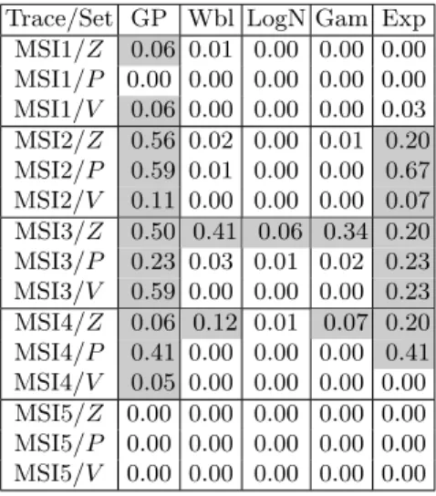
Table 5. P-values of fitting PTBFs, obtained from the KS test. Those larger than the significance level α = 0.05 are in gray boxes.
GP Wbl LogN Gam Exp MSI1 0 0 0 0 0 MSI2 0.03 0.03 0.04 0.07 0.08 MSI3 0.29 0.19 0.17 0.26 0.09 MSI4 0 0.08 0 0.29 0 MSI5 0 0 0 0 0
tribution candidate. Finally, Gam should be the best choice for MSI4 besides Wbl. Different from MSI1 and MSI5, the staircases in the CDFs of MSI2, MSI3 and MSI4 are relatively small, so have the CDFs be possible to fit the distribu-tion candidates. In contrast, MSI1 and MSI5 focus their PTBFs on their basic value (see Figure 2) and hence the PTBFs are hard to fit the tested distribu-tions. As there is a consensus among MSI2, MSI3 and MSI4, we suggest that the Gamma distribution can be used as a marginal distribution-based model for PTBFs, where zeroes can be added to form a complete TBF process. However, this would be a simple model that is able to capture neither the dependence nor the multiplication feature and hence its representativeness is limited.
It is hard to explain why PTBFs exhibit the multiplication feature. One possible cause is that this is an artifact of the trace resolution. For example, MSI4 has a resolution of 300 seconds so all TBFs in the trace are multiples of 5 minutes even if the actual failures did not exhibit this property. However, this explanation does not fully explain the phenomenon in the other four traces since their resolutions are different from their basic values. Therefore in addition to the resolution, there may be other causes that we did not discover due to limited available information in each trace. We argue that this would be an interesting information to be added in the Failure Trace Archive [10]. Since almost PTBFs in all five traces are multiples of a basic value, it is essential to take this feature into account in our failure models.
5
Failure Modeling
This section presents a model for times between failures that is able to capture all the practical features analysed in previous sections, including the simultaneity,
Table 6. Basic values and fractions of PTBFs that are multiples of a basic value. MSI1 MSI2 MSI3 MSI4 MSI5
Basic value (s) 1200 1200 1200 300 100 Fraction 100% 99% 99% 100% 100%
Fig. 3. Illustration of how the model gathers information from its input.
the dependence and the multiplication. The model described in Algorithm 1
receives a TBF process {Ii} as its input and produces a synthetic TBF process
{Si} with those three features, which can be converted into a sequence of failure
events used in performance study.
5.1 General Model
Our failure model in Algorithm 1 consists of three steps. Firstly, we extract
necessary information from the TBF process input {Ii}, where the extraction is
explained in Figure 3. As we indicated in Table 3, the TBF process of a failure trace contains a large number of zeroes due to the simultaneity feature, it is
reasonable to set up a 2-state model: {Ii} goes to state-0 if its value is zero,
otherwise it is with state-1. Once {Ii} falls into a state, we will determine how
long it remains in the state before switching to the other state. For example with a TBF process in Figure 3, we form for state-0 a set Z that contains the lengths of all zero sequences. With respect to state-1, we produce a similar set P with the lengths of all PTBF sequences. We also determine the basis value B of the TBF process that will be used later for the multiplication feature. Furthermore, all PTBFs are collected, divided by B and stored into a set V . With Z, P, V, B, we gather enough information and finish the first step of the model. As the second step, we find the best fitted marginal distribution for Z, P and V , denoted by DistZ, DistP and DistV , respectively. The fitting methodology will be presented later in Section 5.2.
As the last step, we generate {Si} through a main loop. We initialize by
randomly picking a state. Then, we sample a value r, which indicates how many TBFs should be created in this state, by using DistZ or DistP , depending on
the state. With r, the dependence structure of {Si} can be controlled as similar
as that of {Ii}. If the state is state-0, we generate a sequence of r zero values and
Algorithm 1 The failure model.
Input: a TBF process {Ii}.
Output: a synthetic TBF process {Si}.
[Z, P, V, B] = ExtractInf o({Ii}); // Extract necessary information from input
DistZ = F it(Z); DistP = F it(P ); DistV = F it(V ); // Find fitted distributions state = random({0, 1}); N = 0; // Initialize
repeat if state = 0 then r = round(Sampling(DistZ)); SN +1. . . SN +r= 0; else r = round(Sampling(DistP )); for j = 1 to r do SN +j= round(Sampling(DistV )) ∗ B
+[−Res ∗ U niF ]; // Optional end for
end if N = N + r; state = 1 − state;
until N + 1 ≥ desired number of failures;
hence helps to capture the simultaneity feature for {Si}. If the state is state-1,
we generate a sequence of r PTBFs, each is formed by sampling DistV and
multiplying with B to obtain the multiplication feature5. Then, we switch to
state-0 and continue the loop until the desired number of failures is achieved. Indeed, the model operates similarly as a 2-state Markov chain [4], where there is no probability for a state to switch to itself.
5.2 Fitting Methodology
In order to find the best fits for Z, P and V sets, we also apply the maximum likelihood estimation method and the KS test on the five well-known distribution candidates as described in Section 4. Since data are hard to fit any distribution if they contain some specific values that are dominant over other values, as illustrated when we fit PTBFs of MSI1 and MSI5 in Section 4, we carefully check if this happens with the Z, P and V sets. In Table 7, we list top four values that appear in the sets with their frequency. As we can see in most cases, values 1 and 2 are dominant over other values. Therefore, we remove values 1 and 2 out of the fitting process. Furthermore since the applied distribution candidates support a non-negative value domain and we already remove the two 5 Since failures are reported with a resolution, our model also allows to generate
“ac-tual” failure times if one needs by subtracting each generated PTBF an amount of Res ∗ U niF , where Res is the resolution and U niF is the uniform distribution in the range [0, 1].
smallest values out of the sets, which results in 3 as the new smallest value, we decide to shift all remaining values of the sets by 3 units to ease the fitting process. In summary, let X be any from the Z, P and V sets, we will find the best fit for the set Y = {y = x − 3|x ∈ X \ {1, 2}}.
Table 7. Top four values (ordered) appear in the Z, P and V sets. Reading format: a value above and a frequency in percentage below, correspondingly.
Z P V MSI1 (1 2 8 6) (1 2 3 4) (1 2 3 4) (17 8 6 5) (60 21 6 5) (40 11 5 4) MSI2 (1 2 3 25) (1 2 4 3) (1 2 3 4) (30 14 7 5) (37 12 9 7) (15 9 7 7) MSI3 (1 2 9 3) (1 3 10 2) (1 2 5 3) (45 9 9 5) (26 17 13 4) (12 10 6 6) MSI4 (1 2 3 6) (1 2 3 6) (1 2 3 5) (43 13 5 5) (28 15 10 10) (4 3 2 1) MSI5 (1 2 3 4) (1 2 3 4) (1 2 3 4) (24 12 9 6) (63 19 8 4) (26 16 10 6)
Table 8. P-values of fitting Y sets, obtained from the KS test. Those larger than the significance level α = 0.05 are in gray boxes.
Trace/Set GP Wbl LogN Gam Exp MSI1/Z 0.06 0.01 0.00 0.00 0.00 MSI1/P 0.00 0.00 0.00 0.00 0.00 MSI1/V 0.06 0.00 0.00 0.00 0.03 MSI2/Z 0.56 0.02 0.00 0.01 0.20 MSI2/P 0.59 0.01 0.00 0.00 0.67 MSI2/V 0.11 0.00 0.00 0.00 0.07 MSI3/Z 0.50 0.41 0.06 0.34 0.20 MSI3/P 0.23 0.03 0.01 0.02 0.23 MSI3/V 0.59 0.00 0.00 0.00 0.23 MSI4/Z 0.06 0.12 0.01 0.07 0.20 MSI4/P 0.41 0.00 0.00 0.00 0.41 MSI4/V 0.05 0.00 0.00 0.00 0.00 MSI5/Z 0.00 0.00 0.00 0.00 0.00 MSI5/P 0.00 0.00 0.00 0.00 0.00 MSI5/V 0.00 0.00 0.00 0.00 0.00
Table 8 shows the results of fitting Y sets, which indicate that GP seems to be the best fitting candidate. In 11/15 cases, GP results in p-values larger than the significance level α = 0.05. Therefore in these cases, the null hypothesis that Y sets are from the GP distribution cannot be rejected. In addition, though Exp
can also be a good candidate, its p-values are smaller than those of GP in most cases. Hence, we suggest that GP should be the best choice for fitting Y sets. As all distribution candidates result in p-values equal to 0 in the other four cases, we additionally use the KS statistic, also produced by the KS test, to select the best distribution. From Table 9, we again confirm that GP should be a suitable choice for fitting Y sets since its KS statistics are smallest, except for the P set of MSI5. Hence for generality of the model, we propose and use GP as the fitting distribution for Y sets in our study, where the estimated parameters of GP are shown in Table 10.
In conclusion, let X be any from the Z, P and V sets, the fitted distribution DistX of X is determined by the following parameters: percentage of value 1 in
X (p1), percentage of value 2 in X (p2) and GP parameters (a, b). To sample a
value x from DistX, we first sample a value pr from the uniform distribution
over the range [0, 1]. If pr ≤ p1, we assign x = 1, else if p1 < pr ≤ p1+ p2,
x = 2. Otherwise, x = g + 3, where g is sampled from the GP distribution with parameters (a, b).
Table 9. KS statistics of fitting Y sets, obtained from the KS test. Trace/Set GP Wbl LogN Gam Exp
MSI1/P 0.32 0.40 0.41 0.44 0.32 MSI5/Z 0.14 0.27 0.39 0.28 0.22 MSI5/P 0.36 0.33 0.35 0.33 0.44 MSI5/V 0.17 0.32 0.40 0.31 0.28
Table 10. Estimated parameters of GP(a, b), where a and b indicate shape and scale. MSI1 MSI2 MSI3 MSI4 MSI5
Z 0.33 20.82 0.45 46.35 0.45 19.19 -0.75 27.87 0.87 8.04 P -0.17 1.82 -0.08 5.77 0.02 5.31 0.10 3.87 12.54 0.00 V 0.11 12.10 0.23 9.21 0.24 12.53 0.35 302.96 1.07 3.97
6
Validation of the Model
We present in this section our experiments to validate our model. We apply the model to all the traces in Table 1 to generate synthetic failures. The quality of these synthetic failures is evaluated by comparing with the real data. Our evaluation focuses on the simultaneity feature, the dependence structure and the marginal distribution of TBFs. Evaluating the multiplication feature is not necessary because it is guaranteed when we generate PTBFs by sampling the distribution DistV and multiplying with the basic value B (see Algorithm 1).
6.1 Simultaneous Failures
Table 11 describes fractions of simultaneous failures produced by the model. It can be seen that our model controls well this feature since the fractions are close to those of the real data. The quality of generating this feature depends on fitting the Z sets. Successfully fitting the sets, as shown in Tables 8 and 9, helps to control well the number of zeros generated in a TBF process. In case of MSI5, though the p-value of fitting the Z set to GP is 0, its KS statistic is small. Thus, the fitting is acceptable, resulting in a good control of the simultaneity.
Table 11. Fractions of simultaneous failures produced by the model. MSI1 MSI2 MSI3 MSI4 MSI5
Data 97% 93% 75% 73% 95% Model 96% 90% 79% 70% 97%
Table 12. Compare the Hurst parameter between the model and the data, presented as mean ± standard deviation of the five estimators.
MSI1 MSI2 MSI3 MSI4 MSI5 Data 0.60 ± 0.06 0.74 ± 0.14 0.78 ± 0.20 0.70 ± 0.08 0.62 ± 0.08 Model 0.62 ± 0.05 0.76 ± 0.06 0.76 ± 0.18 0.68 ± 0.06 0.54 ± 0.04
6.2 Dependence Structure
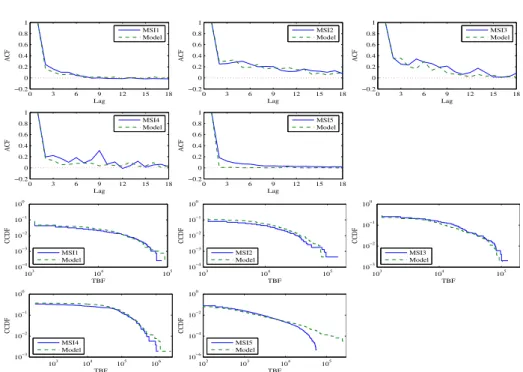
We evaluate the long range dependence feature both via observing an autocor-relation function and estimating the Hurst parameter. The estimation is done similarly as presented in Section 3, i.e. using the SELFIS tool with the five es-timators, namely Aggregate Variance, R/S Statistic, Periodogram, Abry-Veitch and Whittle [9]. As we can see in Figure 4, the autocorrelation of the model fits well to that of the real data, except for the case of MSI5. This is in accordance with the quantitative results of estimating the Hurst parameter in Table 12. It is not strange when the model does not fit MSI5 since we cannot find good fit-ting distributions for the Z, P and V sets of MSI5 as shown in Section 5.2. In contrast for the other cases, the fitting step of the model is well done and thus, the model is able to generate autocorrelated failures.
6.3 Marginal Distribution
One of the first aspects often received the attention of researchers when they analyse or model failures is the marginal distribution. It can be seen that our model is highly representative since it can capture realistic observed features of
0 3 6 9 12 15 18 −0.2 0 0.2 0.4 0.6 0.8 1 Lag ACF MSI1 Model 0 3 6 9 12 15 18 −0.2 0 0.2 0.4 0.6 0.8 1 Lag ACF MSI2 Model 0 3 6 9 12 15 18 −0.2 0 0.2 0.4 0.6 0.8 1 Lag ACF MSI3 Model 0 3 6 9 12 15 18 −0.2 0 0.2 0.4 0.6 0.8 1 Lag ACF MSI4 Model 0 3 6 9 12 15 18 −0.2 0 0.2 0.4 0.6 0.8 1 Lag ACF MSI5 Model 103 104 105 10−4 10−3 10−2 10−1 100 TBF CCDF MSI1 Model 103 104 105 10−4 10−3 10−2 10−1 100 TBF CCDF MSI2 Model 103 104 105 10−3 10−2 10−1 100 TBF CCDF MSI3 Model 103 104 105 106 10−3 10−2 10−1 100 TBF CCDF MSI4 Model 102 103 104 105 10−6 10−4 10−2 100 TBF CCDF MSI5 Model
Fig. 4. Fitting autocorrelation functions and marginal distributions of TBFs.
failures, namely the simultaneity, the dependence and the multiplication. How-ever, its representativeness is even better if it can fit the marginal distributions of real times between failures. Indeed, this is confirmed in Figure 4 where we draw the complementary cumulative distribution functions (CCDFs) of synthetic and real TBFs. The figure shows that our model fits the marginal distribution feature well in four cases. For MSI5, the fitting step does not work finely, which makes the generated TBFs not able to fit the real TBFs well. Nevertheless, the fitting quality of MSI5 is acceptable since the ugly fitting part only occurs when TBFs are larger than 10,000 seconds, which just occupy ∼ 0.2% number of TBFs.
7
Discussion and Related Work
Our study demonstrates that Grid and Cloud infrastructures exhibit proper-ties of simultaneity, dependence and multiplication that must be modeled to accurately capture the characteristics of such systems. Interestingly, the same features are not necessarily present in other types of large-scale systems such as desktop grids and P2P systems. Table 13 measures the occurence of these fea-tures in a number of systems, and highlights systems which clearly exhibit them. Only 2/14 systems exhibit all three features. We so argue that it is essential to develop a specific failure model for systems such as Grids and Clouds.
Many studies have been dedicated to analysing and modeling failures [2, 5, 6, 8, 13–19]. However, most of them focus on servers, high performance clusters,
Table 13. The simultaneity (S), the dependence (D) and the multiplication (M) fea-tures in other systems, expressed by the fraction of simultaneous failures, the Hurst parameter and the basic value, respectively. Grey boxes indicate systems which exhibit the corresponding feature clearly (S <50% and D < 0.6 are not considered).
System Type S D M
UCB Desktop Grid 5% 0.47 No MICROSOFT Desktop Grid 100% 0.52 3600
LRI Desktop Grid 31% 0.56 No DEUG Desktop Grid 5% 0.70 No NOTRE-DAME (host availability) Desktop Grid 90% 0.69 960 NOTRE-DAME (CPU availability) Desktop Grid 99% 0.58 960 PLANETLAB P2P 67% 0.65 900 OVERNET P2P 100% 0.50 1200 SKYPE P2P 100% 0.48 1800 SDSC HPC Cluster 18% 0.53 No LANL HPC Cluster 15% 0.76 60 PNNL HPC Cluster 42% 0.55 100 WEBSITES Web Server 1% 0.63 No LDNS DNS Server 10% 0.56 No
peer-to-peer systems, etc. The few studies dedicated to multi-site systems [6, 8, 18] did not concentrate on modeling the observed features. In [8], a failure model is developed based on fitting real data to distribution candidates, but none of the features observed in this study is captured. Moreover, this model is designed specifically only for GRID’5000 and it is not clear whether it would work for other systems. The model proposed by Yigitbasi et al. [18] studies peaks of failures but not times between failures. Although it studies autocorrelation, it is in terms of failure rates and is not taken into account in their model. Finally, the authors of [6] showed that failures often occur closely in time, in so-called group of failures. The concept of group of failures is close to the simultaneity feature in this paper, and we believe that groups of failures occur due to the vast majority of simultaneous failures as shown in Table 2. Hence, modeling simultaneous failures is more accurate than modeling groups of failures since the information about the times between failures in a group could not be recovered once they are grouped for modeling. Furthermore, the dependence and multiplication features are not taken into account by [6], possibly because it aims at other large-scale systems than multi-site infrastructures.
8
Conclusions and Future Work
This paper demonstrated that failures exhibit simultaneity, dependence and mul-tiplication features, which can have a significant impact on system performance. We proposed a failure model that can capture these features and help research on fault-tolerance mechanisms. The Gamma distribution alone may be used as
a marginal distribution-based model for PTBFs. However, the model from Sec-tion 5 offers much more precision with respect to these three features. It is also flexible as the parameters of GP distributions can easily be tuned. Finally, it ad-dresses the issue of trace resolution and generates “actual” failure times that are not affected by the resolution. Our future work includes adding the unavailabil-ity attribute and using the model to associate failure-awareness for enhancing scheduling performance or resource provisioning in Clouds.
Acknowledgements
This work was partially funded by the Harness project of the Seventh Euro-pean Framework Programme (FP7/2007-2013) under grant agreement number 318521 and by the Netherlands Organization for Scientific Research (NWO) in the context of the Guaranteed Delivery in Grids project.
We would like to acknowledge Lex Wolters for his initial contribution to this work. We regret that he passed away on March 2012.
References
1. J. Beran, “Statistics for Long-Memory Processes”, Chapman & Hall, 1994. 2. J. Chu, K. Labonte, B.N. Levine, “Availability and Locality Measurements of
Peer-to-Peer File Systems”, in ITCom, 2002.
3. D.G. Feitelson, “Workload Modeling for Computer Systems Performance Evalua-tion”, Book Draft, Version 0.32, 2011.
4. W. Feller, “An Introduction to Probability Theory and Its Applications”, 1950. 5. A. Gainaru, F. Cappello, M. Snir, W. Kramer, “Fault Prediction under the
Micro-scope: a Closer Look into HPC Systems”, in SC, 2012.
6. M. Gallet, N. Yigitbasi, B. Javadi, D. Kondo, A. Iosup, D. Epema, “A Model for Space-Correlated Failures in Large-Scale Distributed Systems”, in Euro-Par, 2010. 7. H.E. Hurst, “Long Term Storage Capacity of Reservoirs”, Trans. ASCE, 1951. 8. A. Iosup et al., “On the Dynamic Resource Availability in Grids”, in GRID, 2007. 9. T. Karagiannis et al., “A User-Friendly Self-Similarity Analysis Tool”, 2003. 10. D. Kondo et al., “The Failure Trace Archive: Enabling Comparative Analysis of
Failures in Diverse Distributed Systems”, in CCGRID, 2010.
11. F. Lillo, J. Farmer, “The Long Memory of the Efficient Market”, 2004. 12. J. Myung, “Tutorial on Maximum Likelihood Estimation”, J. Math Psy., 2003. 13. D. Nurmi, J. Brevik, R. Wolski, “Modeling Machine Availability in Enterprise and
Wide-Area Distributed Computing Environments”, in Euro-Par, 2005.
14. D. Oppenheimer, A. Ganapathi, D. A. Patterson, “Why do Internet Services Fail, and What Can Be Done about It?”, in USITS, 2003.
15. A. Pecchia, D. Cotroneo, Z. Kalbarczyk, R.K. Iyer, “Improving Log-Based Field Failure Data Analysis of Multi-Node Computing Systems”, in DSN, 2011. 16. R.K. Sahoo, M.S. Squillante, A. Sivasubramaniam, Y. Zhang, “Failure Data
Anal-ysis of a Large-Scale Heterogeneous Server Environment”, in DSN, 2004.
17. B. Schroeder, G.A. Gibson, “A Large-Scale Study of Failures in High-Performance-Computing Systems”, in DSN, 2006.
18. N. Yigitbasi, M. Gallet, D. Kondo, A. Iosup, D. Epema, “Analysis and Modeling of Time-Correlated Failures in Large-Scale Distributed Systems”, in GRID, 2010. 19. Z. Zheng et al., “3-Dimensional Root Cause Diagnosis via Co-Analysis”, 2012.