Measurement and modelling of solid apparition temperature for the CO2 - H2S - CH4 ternary system

HAL Id: hal-02452603

https://hal.archives-ouvertes.fr/hal-02452603

HAL is a multi-disciplinary open access archive for the deposit and dissemination of sci-entific research documents, whether they are pub-lished or not. The documents may come from teaching and research institutions in France or abroad, or from public or private research centers.

L’archive ouverte pluridisciplinaire HAL, est destinée au dépôt et à la diffusion de documents scientifiques de niveau recherche, publiés ou non, émanant des établissements d’enseignement et de recherche français ou étrangers, des laboratoires publics ou privés.

Measurement and modelling of solid apparition

temperature for the CO2 - H2S - CH4 ternary system

Pascal Théveneau, Rémi Fauve, Christophe Coquelet, Pascal Mougin

To cite this version:

Pascal Théveneau, Rémi Fauve, Christophe Coquelet, Pascal Mougin. Measurement and modelling of solid apparition temperature for the CO2 - H2S - CH4 ternary system. Fluid Phase Equilibria, Elsevier, 2020, 509, pp.112465. �10.1016/j.fluid.2020.112465�. �hal-02452603�

Measurement and modelling of solid apparition temperature for the CO

–

H

S – CH

ternary system

Pascal Théveneau1, Rémi Fauve1, Christophe Coquelet1*, Pascal Mougin2

1 Mines ParisTech, PSL University, CTP – Centre of Thermodynamics of Processes 35, rue Saint Honoré 77305 Fontainebleau Cedex France

2 : IFP Energies nouvelles, 1 et 4 avenue de Bois-Préau, 92852 Rueil-Malmaison, France

Abstract:

In order to develop a new process to eliminate acid gases from natural gas, it is important to consider phase

equilibrium properties. New solid-liquid equilibrium data were determined concerning the ternary system

CO2 + H2S + CH4. The experimental technique is based on visual synthetic method. The new experimental

data were compared to predictions given by the Predictive Peng-Robinson equation of state (PPR78),

PSRK UNIFAC, Peng-Robinson with Huron-Vidal mixing rules and GERG 2008 models coupling with

classical approach or Jager and Span for solid phase. The results have shown that the model selected for the

fluid phase has more impact that the model considered for the solid phase. New binary interaction

parameters of Peng-Robinson equation of state were fitted only on our experimental data and it was found

that the obtained values are very different from the value used for Vapor Liquid Equilibrium computation.

Key words: Solid formation; Ternary mixture; CO2; H2S; CH4,Data treatment

2

1. Introduction

In the past three decades the share of natural gas in the world panorama has been appreciably growing,

to almost one quarter of the energy used worldwide. This trend is expected to increase in the future since a

number of natural gases and gas condensates fields have been discovered around the world. In addition,

natural gas is an energy carrier with a lower carbon footprint than coal or oil. However, this development

will depend on the progress made in technologies allowing access to sour gases contaminated reserves (40%

of the world’s gas reserves). In some cases, the amount of hydrogen sulfide in natural gas can be greater than 30%, and natural gas should be clear of this compound and other acid gases (mercaptan, carbon

dioxide, carbon disulfide, carbonyl sulfide) before its transport.

The technologies currently employed in most industrial plant to remove acid gases are based on

chemical or physical absorption with solvents [1]. Since these solvents need heat to be regenerated between

each absorption, the higher the concentration of acid gases is, the lower the profit. In other hand, some

cryogenic process for bulk hydrogen sulfide (H2S) or carbon dioxide (CO2) removal from very sour gases

has been developed. The kind of process, involving treating the raw gas by cryogenic distillation, has the

advantage of producing sweetened gas. This process has high energetic efficiency and allows the

minimisation of hydrocarbons losses. However, at low temperature, solid phase should appear. As an

example, hydrates were found to develop under some operating conditions in the Lacq pilot unit [2]. Such

solid phase formations are highly undesirable as they decrease the efficiency of the plant, but mainly they

can plug the pipes and eventually damage the installations. In other hand, the crystallization of a compound

may be desirable; for example, there are CO2 capture processes that use fluid-solid equilibrium. Petroleum

industry needs reliable and accurate vapor-liquid and liquid-solid equilibrium data for mixtures of

hydrocarbons and acid gases in order to develop accurate models for calculating thermodynamic properties

of natural gas requested for plants design.

MINES ParisTech fluid thermodynamic laboratory has previously developed specific apparatus and

protocols in order to carry on phase equilibrium for systems with high level of H2S. We can cite the work

published by Dicko et al. [3] on the study of phase behaviour on binary systems composed with H2S and

propane, n-butane and pentane, and the work published by Coquelet et al. [4] on the phase diagram of the

binary system CH4 + H2S from 186 to 313 K.

composed with CO2 + H2S + CH4 and their modelling with classical equations of state (EoS). The

knowledge of this temperature is very important for the determination of optimal operating condition of

pilot plants. The experimental principle is presented in section 2 and the results are presented and analysed

in section 3.1. An attempt at modelling the data with different EoS was carried out with and without fitted

binary interaction parameters (BIP). The method and analysis are presented in section 3.2.

2 Experimental principle

For the experiments in the present study, visual synthetic method was considered. Five compositions

of the ternary mixture CO2 + H2S + CH4 were considered. The measurements were performed using an

in-house specially designed apparatus allowing the visual detection of a solid phase formation.

2.1 Materials

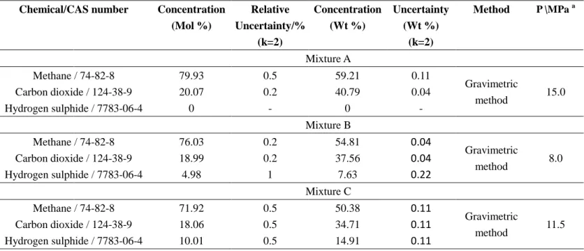
The considered mixtures, presented in Table 1, were purchased from AIR PRODUCTS. In the Table 1,

uncertainties given by the supplier concerning the preparation of the mixtures are presented.

[Table 1]

Table 1. Chemical sample (Air Product certified values, standard

ISO9001:2000

Chemical/CAS number Concentration (Mol %) Relative Uncertainty/% (k=2) Concentration (Wt %) Uncertainty (Wt %) (k=2) Method P \MPa a Mixture A Methane / 74-82-8 79.93 0.5 59.21 0.11 Gravimetric method 15.0 Carbon dioxide / 124-38-9 20.07 0.2 40.79 0.04 Hydrogen sulphide / 7783-06-4 0 - 0 - Mixture B Methane / 74-82-8 76.03 0.2 54.81 0.04 Gravimetric method 8.0 Carbon dioxide / 124-38-9 18.99 0.2 37.56 0.04 Hydrogen sulphide / 7783-06-4 4.98 1 7.63 0.22 Mixture C Methane / 74-82-8 71.92 0.5 50.38 0.11 Gravimetric method 11.5 Carbon dioxide / 124-38-9 18.06 0.5 34.71 0.11 Hydrogen sulphide / 7783-06-4 10.01 0.5 14.91 0.11

4 Mixture D Methane / 74-82-8 68.02 0.5 46.42 0.12 Gravimetric method 6.1 Carbon dioxide / 124-38-9 17.01 0.5 31.85 0.12 Hydrogen sulphide / 7783-06-4 14.97 0.5 21.72 0.12 Mixture E Methane / 74-82-8 63.95 0.5 42.49 0.12 Gravimetric method 4.9 Carbon dioxide / 124-38-9 16.04 0.5 29.24 0.12 Hydrogen sulphide / 7783-06-4 20.01 0.5 28.27 0.12 a

Pressure of the mixture at 288.15 K

2.2 Apparatus description

An in-house developed apparatus based on a visual static-synthetic method is used in this work to

perform the solid phase formation’s temperature measurement (Figure 1). The equilibrium cell (length

around 19mm, internal diameter around 12.7 mm and internal volume around 2.4 cm3) is comprised of a

horizontal sapphire tube, which contains the mixture and a few agitation glass beads, sealed by two

titanium flanges respectively on the left and the right. The left flange is connected to a platinum resistance

thermometer probe (Pt100, 100 Ω). The right flange is connected a pressure transducer and a loading valve.

The connected loading tube is linked, through a three-way valve, with the mixture storage bottle and a

vacuum pump used for discharging, degassing and evacuation operations of the residual substance in the

circuit. The equilibrium cell is immersed into a water thermoregulated liquid bath that provides and keeps

the desired operating temperature within ± 0.01 K.

The temperature is measured by a platinum probe (100 Ω). The temperature probe was calibrated

against a standard probe (25 Ω, TINSLEY, U.K., Model 5187 SA) connected to a precision Ohmmeter

(AGILENT, Model 34420A). Temperature calibration uncertainty is estimated to be , in the temperature scale 188.48 K to 223.55 K.

The pressure is measured by a pressure transducer (SEDEME, Model MD200) connected to a display

data acquisition unit (AGILENT, Model 34970A). During the experiments, the pressure transducer is

thermoregulated at 308.15 K. The pressure transducer was calibrated using a deadweight tester

(DESGRANGES & HUOT, Model 5202S CP). Pressure calibration uncertainties are estimated to be

. Thermometers and pressure transducers are connected to a digital data display unit (Agilent, model 34420A) connected to a computer.

[Figure 1]

Figure 1: Picture of the equilibrium cell.

2.3 Experimental procedure

The cell and loading circuit are placed under vacuum at ambient temperature, then the cell is

immersed in a thermostat liquid bath at 208.15 K. With the cell’s loading valve closed, the mixture is

allowed in the circuit by opening the safety valve on the mixture storage bottle and the valve connected to

the loading tube. The cell’s loading valve is then carefully opened to let the mixture fill the cell. The loading valve is closed when the cell is completely filled with the mixture.

When thermodynamic equilibrium is reached in the cell, the mixture is agitated by gently swinging the

cell from left to right to move the glass beads inside the cell. The cell is maintained immersed in the

thermostat liquid bath during the agitation process. Then the cell is extracted from the thermostat liquid

bath for observation. If no solid phase is detected, the temperature of the thermostat liquid bath is lowered,

or raised otherwise. The observation is done following an increase and a decrease of temperature to better

identify the temperature of solid phase formation in the mixture. During the experiment, aside from the

formation of the solid phase, a single phase was visually identified in the cell. Following our experimental

Platinum probe Loading

valve Loading circuit To pressure transducer Sapphire tube Glass beads

6

procedure, we have defined an uncertainty of temperature measurement which takes into account the

variation of temperature between the moment where a solid phase is observed and the moment where there

is no solid phase. The maximum “experimental procedure “uncertainty is less than u(T)=1.2 K.

Only for mixture E the detection of solid phase was not very clear, this is why we have repeated the

measurement of solid formation only for this mixture. Repeatability measurement consists of removing the

mixture in the equilibrium cell and loading a new one.

3. Results and discussion

3.1 Experimental results

The experimental temperature and pressure of solid phase formation for five compositions of the CO2 +

H2S + CH4 ternary system are reported in Table 2 and plotted in Figure 2. A second measurement was done

with mixture E, as a repeatability test. The results are very similar, when taking into account the

experimental uncertainties. Hereinafter, mixture E will refer to the average of these two measurements.

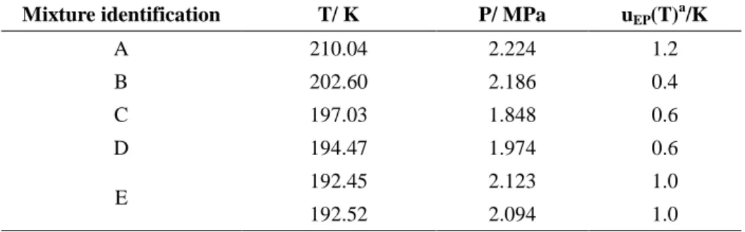
Table 2: Experimental Temperature of solid phase formation for the different mixtures studied, ucal(T)=0.02K, ucal(P)=0.005 MPa.

Mixture identification T/ K P/ MPa uEP(T)a/K

A 210.04 2.224 1.2 B 202.60 2.186 0.4 C 197.03 1.848 0.6 D 194.47 1.974 0.6 E 192.45 2.123 1.0 192.52 2.094 1.0 a

Uncertainty due to our experimental procedure

[Figure 2]

Figure 2 : Variation of acid gas composition as a function of the temperature of solid phase formation (: CO₂, ◇: H2S) in the CO2 + H2S + CH4 ternary mixture. Solid lines: second degree polynomials fitted

on the data. Error bar: values from Table 2.

In Figure 2, the temperature of solid phase formation for the mixture B ( ) looks a bit out of trend, although the measurement for this mixture has not presented any particular problem.

This lack of precision can be explained by a higher uncertainty on H2S mole fraction in mixture B, as

provided by AIR PRODUCTS (see Table 1).

This behaviour can be reproduced by correlating the temperature of solid phase formation with a ratio

of the different mole fractions of the components of the system. In Table 3 are presented the composition

and the ratios between each component. The ratios

can be averaged over the different mixtures at

0.00 0.05 0.10 0.15 0.20 0.25 190 195 200 205 210 215 M ol e fr ac ti on Temperature /K

8

, with a relative deviation of

, so the ratio can be considered constant for the different mixtures. The Figure 3 shows that the temperature of solid phase

formation can be well correlated ( and ) with the ratio by an exponential function (Eq. 1).

(1)

With , and . The authors think that for other values of , the same behavior will occur. This assertion could be tested with additional measurements.

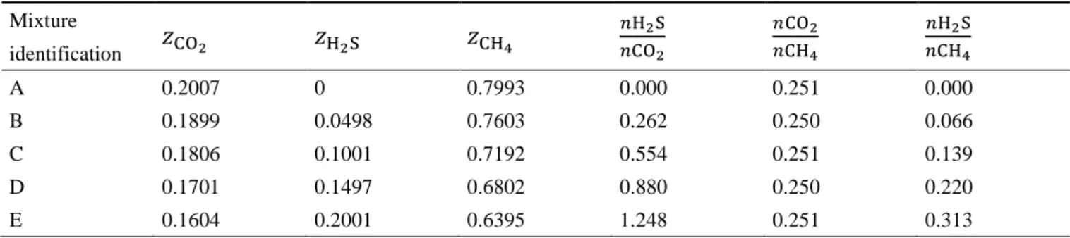
[Table 3]

Table 3: Mixture compositions and mole fractions ratios

Mixture identification

Figure 3 : Temperature of solid phase formation for different values of

.

3.2 Thermodynamic modelling

Model for solid-liquid equilibrium calculation

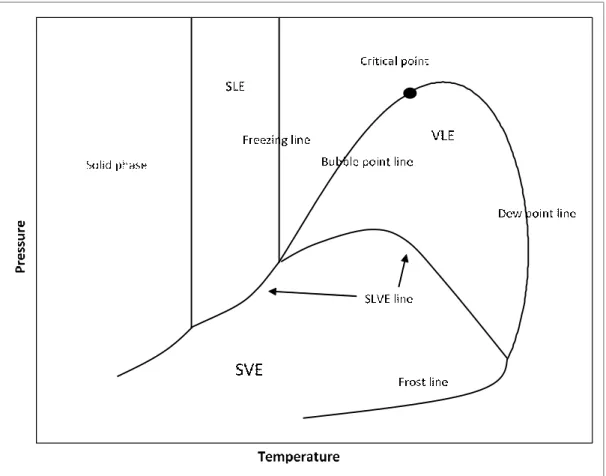
The Figure 4 represents the classical PT envelop of a system including solid phase. The chosen

approach for modelling the temperature of the solid phase formation is the equilibrium condition for a

solid-liquid system written in terms of the fugacities of the solid-forming component, which can be

assumed as pure CO2 (Eq. 2). For the other chemical species, we assume that they are in a fluid state.

(2)

where is the temperature, is the pressure, is the fluid phase concentration. The fugacity of the solid phase can be calculated (Eq. 3) from the model developed for the fluid-solid equilibrium described by

Prausnitz et al. [5], page 635.

₍₃₎

Where the suffix is the reference state, is the molar fusion enthalpy of pure CO2 in its reference state given by Gas Encyclopedia [6] and is the fusion temperature of pure CO2.

10

Figure 4: Classical PT envelop of a mixture including solid phase. VLE: Vapor-liquid Equilibrium, SLE: Solid-liquid equilibrium, SVE: Solid-vapor equilibrium, SLVE:

Solid-liquid-vapor equilibrium.

It has been chosen to compute the fugacity of the fluid phase with different predictive EoS: Predictive

Peng-Robinson EoS (PPR78) [7], Predictive Soave-Redlich-Kwong EoS UNIFAC (PSRK UNIFAC) [8],

implemented in Simulis® Thermodynamics Software from Prosim (France), Peng-Robinson with

Huron-Vidal mixing rules (PR-HV) [9] and GERG 2008 EoS [10] implemented in REFPROP (version 10.0)

from NIST. The PR-HV EoS used Huron-Vidal mixing rules with the NRTL-V activity model for the Gibbs

free energy; the parameters of this activity approach have been obtained using both VLE and VLLE data

(binary and ternary subsystems). The details of the model have been given in [11] in the form of application

case 1.

One objective of this work is to compare the performance of these four predictive models to correlate

the experimental data presented in this paper. For each system composition and an initial temperature, the

calculated using one of the chosen EoS, i.e. PPR78, PSRK, PR-HV and GERG 2008 EoS. The solid CO2

fugacity is calculated using the fluid-solid equilibrium model (Eq 2). Then, for each system composition,

the temperature that satisfies the isofugacity condition is obtained through the minimization of the

difference between the fluid phase fugacity and the solid CO2 fugacity, using the non-linear Generalized

Reduced Gradient (GRG) algorithm.

Results are presented on Table 4 and plotted in Figure 5. Mean Absolute Deviation (MAD) and Mean

Relative Deviation (MRD), applied on temperatures, are defined by Eqs. (4) and (5) respectively.

(4)

(5)

As we can see, the PR-HV EoS gives the best results in comparison with the prediction obtained using

the two cubic EoS, PPR78 and PRSK, and the GERG approach. The binary parameters of the Huron-Vidal

mixing rules have been obtained previously from regression work on binary systems: CH4 + CO2, CH4 +

H2S, CO2 + H2S [12]. Among the other three models, the GERG approach is the one that gives the lowest

deviations (mean deviation close to 4.1 K), the PSRK EoS shows a deviation about 10 K and PPR78 gives

the larger deviation (21 K). The two later show also the larger deviations when the H2S content increases.

To confirm the impact of the fluid model on these phase equilibria, we also verified the ability of the

PR-HV equation to reproduce the fluid phase diagrams of the different binary as well as the ternary. The

figures 6, 7 and 8 below illustrate this ability. In the case of the ternary system, the PR-HV model makes it

possible to predict the classical liquid-vapor behavior as well as the liquid-liquid situation, which is not the

case with a classical PR model.

12

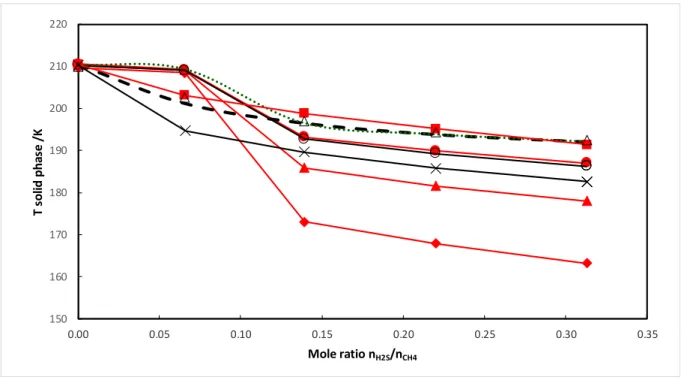
Figure 5 : Temperature of solid phase formation for different values of

.

Δ

×



calculated using GERG 2008 EoS with Eq. 3 for the calculation of solid CO2 fugacity. o: calculated using

GERG 2008 EoS with Jager and Span model [17] for the calculation of solid CO2 fugacity. Green dotted

line: calculation using Peng Robinson EoS with adjusted BIP. Black dashed line: calculation using Peng Robinson EoS with adjusted BIP and new composition of mixture B.

150 160 170 180 190 200 210 220 0.00 0.05 0.10 0.15 0.20 0.25 0.30 0.35 T so lid p h as e / K Mole ratio nH2S/nCH4

Figure 6 : Fluid phase diagrams of CH4 + CO2 system at low temperature [13]

.

experimental data and lines are PR-HV model.

[Figure 6]

Figure 7 : Fluid phase diagrams of CH4 + H2S system at low temperature

.

14

[Figure 7]

Figure 8 : Fluid phase diagrams of CO2 + H2S system at low temperature

.

data [14] and lines are PR-HV model.

[Figure 8]

Figure 9 : Fluid phase diagrams of CH4 + CO2 + H2S system at low temperature

.

experimental data [15], solid lines are PR-HV model and dot line are PR model with conventional binary parameters [16].

[Figure 9]

We can also observe that the prediction of the temperature of solid formation for the mixture without

H2S is not very good. Consequently, we have decided to change the model for the calculation of fugacity of

the CO2 at its solid state. Jäger and Span [17] has proposed in 2012 an EoS to compute directly the Gibbs

energy of the CO2 for temperature below its triple point temperature. The advantage is that we do not have

to extrapolate the prediction of CO2 liquid fugacity below CO2 triple point temperature. Eq. (6) gives the

expression of the solid CO2 fugacity.

(6)

The reference state for the Gibbs Energy model considered here is the ideal gas at and . It is calculated using GERG 2008 EoS. The results are presented in Table 4 and Figure 5. We can conclude that it does not improve the prediction of the temperature of solid formation.

Consequently, in order to improve the data treatment, we have decided to use the PR EoS for the liquid

phase and to adjust the BIP using our experimental data. PR-HV model was consider to define the fluid

state for each experimental data.

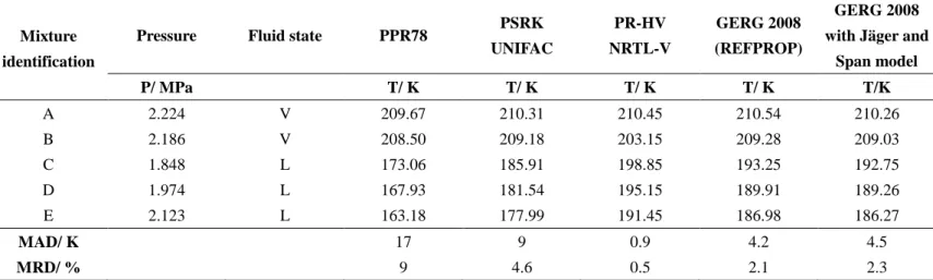
[Table 4]

Table 4: Prediction of temperature of solid formation by the four predictive models using Eq. 2 for the calculation of CO2 fugacity at its solid state.

Mixture identification

Pressure Fluid state PPR78 PSRK UNIFAC PR-HV NRTL-V GERG 2008 (REFPROP) GERG 2008 with Jäger and

Span model P/ MPa T/ K T/ K T/ K T/ K T/K A 2.224 V 209.67 210.31 210.45 210.54 210.26 B 2.186 V 208.50 209.18 203.15 209.28 209.03 C 1.848 L 173.06 185.91 198.85 193.25 192.75 D 1.974 L 167.93 181.54 195.15 189.91 189.26 E 2.123 L 163.18 177.99 191.45 186.98 186.27 MAD/ K 17 9 0.9 4.2 4.5 MRD/ % 9 4.6 0.5 2.1 2.3

In conclusion, we can consider that there is no impact of the model considered for the solid phase but the

selection of the equation of state for the fluid phase has a non-negligible impact.

16

In this section we will use our new experimental data and adjust parameters of a cubic EoS used to

calculate the fugacity of fluid phase. BIP were considered in the Peng Robinson EoS [18] used to compute

the fugacity of the fluid phase and were optimized to minimize the deviation between experimental and

calculated temperatures, using an algorithm based on simulated annealing methods (Salamon et al. [19] and

van Laarhoven et al. [20]), which flowchart is presented in Figure 6. This algorithm was selected because

of its ability to avoid getting stuck in local optima, thus to better explore the solutions space. Eq. (7)

presents the selected objective function.

(7)

The optimal values of the three BIP are presented in Table 5 and the resulting temperatures are presented in

Table 6 and plotted in Figure 5.

[Table 5]

Table 5: Optimal BIP values

BIP New value Sandler [16]

0.1781 0.097

0.1212 0.09

[Table 6]

Table 6: Results for EoS with optimal BIP

Mixture identification PR EoS T /K A 210.45 B 209.38 C 196.57 D 193.89 E 192.12 MAD/ K 1.7 MRD/ % 0.85

As expected the results are better after adjustment of BIP using our experimental data and close to the

results obtained using the PR-HV EoS. We observe a strange calculation for the mixture B. Regarding the

certificate given by AIR PRODUCTS concerning this chemical, we can see that the relative uncertainty on

H2S mole fraction is the most important. So we try to repeat the calculation by considering a new

composition of the mixture. If we consider the mixture B with a new molar composition , and if we consider that the fluid phase is a liquid phase, we calculate a temperature close to the temperature measured (201.21 K, see Figure 3). The deviation from original H2S

mole fraction is around 20% which seems to be very important. One reason of such deviation can be the

inability of the PR EoS to generate accurate PT envelop for such mixture composition and consequently

calculates temperature of solid formation with some deviation. This may explain why there is a

non-negligible deviation between our experimental data and the model calculation also after adjustment of

BIP. It is important to notice that the PR HV model predict very well the temperature of solid apparition.

Certainly one reason is that the PR HV is more accurate to predict the phase diagram of the fluid phase (i.e.

VLE) as it is composed with Huron Vidal mixing rules involving NRTL activity coefficient model. This

point is confirmed by analysis of BIP values after their adjustment. In effect, as can be seen on Table 5, the

values of the BIP are different to the values available in the literature (Sandler [16], values from

DECHEMA) and one can notice their high values. It is due to the fact that classical mixing rule is not

adapted for such condition of phase equilibrium. Also, we have presented in Figure 5 the results obtained

using Sandler’s parameters and they are very close to the values calculated using PSRK model. It confirms that PPR78 model prediction and the temperature dependency of the BIP of this model is not adapted for

18

such phase equilibrium calculation. Consequently, if classical mixing rule is selected, it may be wise to use

BIP adjusted from vapor-liquid equilibrium data and to adjust BIP with a mixing rule on molar co-volume

if users wants to remain constant the value of BIP for attractive parameter.

[Figure 10]

4. Conclusion

New temperatures of solid formation were measured for 5 mixtures composed with

CO

, H

S and

CH

solid phase formation and the ratio for a constant ratio , and vice-versa. Two EoS based on Group Contribution approach (PPR78, PSRK) were tested to predicted the CO2 freezing temperature and

the results reveals that deviations are important when the mixture contains H2S. We have also used a

semi-empirical EoS developed for natural gas (GERG-2008 EoS) and the results are improved. The best

results have been obtained with the PR-HV EoS which has been developed to well suit the behaviour of

CH4/ CO2/H2S fluid phase equilibrium.

We have examined the influence of the solid fugacity model of the CO2 with the Jäger and Span

mode however the impact is negligible.

Adjustment of cubic EoS BIP leads to a better representation of the data but not for mixture B

(calculations are strongly dependent on the mixture composition) but the values of BIP adjusted are very

different from the one obtained by considering the VLE data. Strategy for SLE computation using cubic

20

5. REFERENCES

[1] A.L. Kohl, R. Nielsen, (1997) Gas Purification, 5th edition, gulf professional publishing, ISBN : 9780884152200

[2] F. Lallemand, F. Lecomte, C. Sreicher (2005) Highly sour gas processing: H2S bulk removal with the SPREX process, IPTC 10581.

[3 . ic o , C. Coquelet, P. Theveneau, P. Mougin (2012) Phase equilibria of H2S-Hydrocarbons (propane, n-butane and n-pentane) binary system at low temperature, J. Chem. Eng. Data, 57, 1534-1543

[4] C. Coquelet, A. Valtz, P. Stringari, M. Popovic, D. Richon, P. Mougin (2014) Vapour – Liquid Equilibrium Data for the Hydrogen Sulphide + Methane System at Temperatures from 186 to 313 K and Pressures up to about 14 MPa, Fluid Phase Equilibria, 383, 94-99.

[5] J.M. Prausnitz, R.N. Lichtenthaler, E.G. De Azevedo (1998) Molecular Thermodynamics of Fluid-Phase Equilibria, Prentice Hall; 3rd edition.

[6] Air Liquide: Gas Encyclopedia, 1976

[7] J.N. Jaubert, R. Privat & F. Mutelet (2010). Predicting the phase equilibria of synthetic petroleum fluids with the PPR78 approach. AIChE journal, 56(12), 3225-3235.

[8] T. Holderbaum & J. Gmehling (1991). PSRK: A group contribution equation of state based on UNIFAC. Fluid Phase Equilibria, 70(2-3), 251-265.

[9] M.J. Huron & J. Vidal (1978). New mixing rules in simple equations of state for representing vapour-liquid equilibria of strongly non ideal mixtures. Fluid Phase Equilibria 3, 255-271

[10] O. Kunz, W. Wagner (20012) The GERG-2008 Wide-Range Equation of State for Natural Gases and Other Mixtures: An Expansion of GERG-2004, J. Chem. Eng. Data, 57, 3032-3091.

[11] J.C. de Hemptinne, J.M. Ledanois, P. Mougin, A. Barreau, (2011) Select thermodynamic models for process simulation- A Practical Guide to a Three Steps Methodology, Technip Edition,

https://books.ifpenergiesnouvelles.fr/ebooks/thermodynamics/studies/06_Liquefin_2009_August.html

[12] C. Coquelet, A. Valtz, P. Stringari, M. Popovic, D. Richon, P. Mougin. (2014) Phase equilibrium data

for the hydrogen sulphide + methane system at temperatures from 186 to 313 K and pressures up to about

[13] S. Mraw, S. Hwang, R. Kobayashi. (1978) Vapor-Liquid Equilibrium of the CH4 - CO2 System at Low Temperatures, J. Chem. Eng. Data, 23(2), 135-139.

[14] D. Sobocinski, F. Kurata. (1959) Heterogeneous Phase Equilibria of the Hydrogen Sulfide - Carbon Dioxide System, AIChE J., 5(4), 545-551.

[15] H.-J. Ng, D. Robinson and A.-H. Leu (1985). Critical phenomena in a mixture of methane, carbon dioxide and hydrogen sulfide, Fluid Phase Equilbrium, 19, 273-286

[16] S. Sandler (2006) Chemical, Biochemical, and Engineering Thermodynamics, 4th edition, John Wiley & Sons, ISBN: 0471661740

[17] A. ger & R. Span (2012). Equation of state for solid carbon dioxide based on the Gibbs free energy. Journal of Chemical & Engineering Data, 57(2), 590-597.

[18] D. Y. Peng & D. B. Robinson (1976). A new two-constant equation of state. Industrial & Engineering Chemistry Fundamentals, 15(1), 59-64.

[19] P. Salamon, P. Sibani & R. Frost (2002). Facts, conjectures, and improvements for simulated annealing (Vol. 7). Siam.

[20] P. J. Van Laarhoven & E.H. Aarts (1987). Simulated annealing. In Simulated annealing: Theory and applications (pp. 7-15). Springer, Dordrecht.

22

List of Tables

Table 1. Chemical sample (Air Product certified values, standard

ISO9001:2000

Table 2: Experimental Temperature of solid phase formation for the different mixtures studied, ucal(T)=0.02K, ucal(P)=0.005 MPa.

Table 3: Mixture compositions and mole fractions ratios

Table 4: Prediction of temperature of solid formation by the four predictive models using Eq. 2 for the

calculation of CO2 fugacity at its solid state.

Table 5: Optimal BIP values

Table 6: Results for EoS with optimal BIP

List of Figures

Figure 1: Picture of the equilibrium cell.

Figure 2 : Variation of acid gas composition as a function of the temperature of solid phase formation (: CO2, ◇: H2S) in the CO2 + H2S + CH4 ternary mixture. Solid lines: second degree polynomials fitted on the data. Error bar: values from Table 2.

Figure 3 : Temperature of solid phase formation for different values of . △: our data. Solid line: our

correlation.

Figure 4: Classical PT envelop of a mixture including solid phase. VLE: Vapor-liquid Equilibrium, SLE:

Solid-liquid equilibrium, SVE: Solid-vapor equilibrium, SLVE: Solid-liquid-vapor equilibrium.

Figure 5: Temperature of solid phase formation for different values of .

Δ: our experimental data. ×: Calculated using PR EoS with Sandler [16] parameters. : calculated data using PPR78 EoS. ▲: calculated data using PSRK UNIFAC EoS. ■: calculated data using PR-HV EoS. : calculated using GERG 2008 EoS with Eq. 3 for the calculation of solid CO2 fugacity. o: calculated using GERG 2008 EoS with Jager and Span model [17] for the calculation of solid CO2 fugacity. Green dotted line: calculation using Peng Robinson EoS with adjusted BIP. Black dashed line: calculation using Peng Robinson EoS with adjusted BIP and new composition of mixture B.

[13] and lines are PR-HV model.

Figure 7: Fluid phase diagrams of CH4 + H2S system at low temperature. Symbols are experimental data

[12] and lines are PR-HV model.

Figure 8 : Fluid phase diagrams of CO2 + H2S system at low temperature. Symbols are experimental data

[14] and lines are PR-HV model.

Figure 9 : Fluid phase diagrams of CH4 + CO2 + H2S system at low temperature. Symbols are

experimental data [15], solid lines are PR-HV model and dot line are PR model with conventional binary

parameters [16].