A Volatility-Driven Asset Allocation (VDAA)

CAHIER DE RECHERCHE DE DRM

N° 2010-13

A Volatility-Driven Asset Allocation (VDAA) Laurent Michel, Thierry Michel and Christophe Morel

Abstract

This article advocates a systematic rebalancing process –Volatility-Driven Asset Allocation or VDAA – for dynamically managing the strategic asset allocation. The goal of the suggested algorithm is to adjust the asset exposures so as to reflect the assumptions investors used when determining their strategic allocation, in terms of balance between risk contributions and expected returns. Such an idea makes sense from the economic point of view of a risk-adverse investor who wishes to achieve a smooth long-run performance. The stable risk contribution is determined by a long-run target, with short-term deviations from this target driving the rebalancing of the portfolio exposure. Rebalancing between asset classes allows smoothing the global volatility of the portfolio by decreasing exposure in asset classes yielding temporarily higher risk contributions and by increasing weight in asset classes with temporarily lower risk contributions. Both our backtests and robustness study demonstrate that this risk rebalancing strategy is superior in terms of information ratio to traditional rebalancing rules.

A Volatility-Driven Asset Allocation

(VDAA)

L

M

,

T

M

,

C

M

Laurent Michel is senior portfolio manager in the Tactical Asset Allocation department at

Lombard Odier Investment Managers, in Geneva, Switzerland. l.michel@lombardodier.com

Thierry Michel is senior portfolio manager in the Tactical Asset Allocation department at

Lombard Odier Investment Managers, in Geneva, Switzerland, and associate professor at ESCP-EAP, France. t.michel@lombardodier.com.

Christophe Morel is head of Tactical Asset Allocation at Lombard Odier Investment

Managers, in Geneva, Switzerland, and research associate at Paris-Dauphine University, France. ca.morel@lombardodier.com

Abstract

This article advocates a systematic rebalancing process –Volatility-Driven Asset Allocation or VDAA – for dynamically managing the strategic asset allocation. The goal of the suggested algorithm is to adjust the asset exposures so as to reflect the assumptions investors used when determining their strategic allocation, in terms of balance between risk contributions and expected returns. Such an idea makes sense from the economic point of view of a risk-adverse investor who wishes to achieve a smooth long-run performance. The stable risk contribution is determined by a long-run target, with short-term deviations from this target driving the rebalancing of the portfolio exposure. Rebalancing between asset classes allows smoothing the global volatility of the portfolio by decreasing exposure in asset classes yielding temporarily higher risk contributions and by increasing weight in asset classes with temporarily lower risk contributions. Both our backtests and robustness study demonstrate that this risk rebalancing strategy is superior in terms of information ratio to traditional rebalancing rules.

The recent financial turmoil has underlined the challenges investors face when implementing an asset allocation policy, reminding them that asset weights is misleading about the global risk of a portfolio. When comparing asset classes, the relevant metric is obviously not weight but risk. An asset allocation based on exposure might give the impression that a portfolio is fairly balanced, which might be true in a low volatility regime. As soon as asset volatility spikes, however, the global risk borne by the portfolio is mostly determined by its riskier assets. So the portfolio risk may become largely stronger than the risk budget defined in its strategic asset allocation and far from consistent with the risk the investor’s governance agreed when deciding the long-term investment policy.

The frontier between strategic asset allocation (SAA hereafter) and tactical asset allocation (TAA) is narrow. TAA is supposed to add value compared to the strategic benchmark. But it is also the role of TAA to dynamically adjust exposure in risky assets in order to maintain the ex ante drawdown in consistency with the SAA risk budget. Our risk-driven approach (Volatility-Driven Asset Allocation or VDAA) consists in keeping constant the portfolio volatility – whenever possible – by adjusting weights by de-leveraging in periods of high volatility and leveraging in periods of low volatility. From a theoretical point of view, this volatility-driven strategy is based on the portfolio separation theorem suggesting that a benign-neglect behavior is not justified as the optimal asset allocation depends on the investor tolerance of risk. As soon as there is a change in the risk environment, the efficient frontier is subject to modification, and the optimal asset allocation is supposed to be realigned with the investor’s risk aversion. This adjustment is all the more relevant as volatility is persistent and exhibits memory, meaning that periods of high (respectively low) volatility tend to be followed by periods of high (respectively. low) volatility. This is the reason why even after a jump in volatility it might still be optimal for an investor to reduce significantly his exposure to risky assets.

This paper is at the crossroads of two topics in academic literature: the economic value of volatility-timing and the optimal rebalancing strategy.

Merton [1973] was the first to argue that, investors should alter their portfolio holdings to take advantage of time-varying investment opportunities. More recently, some academic studies (Fleming and al. [2001, 2003], Gomes [2003], Liu and al. [2003], Marquering and Verbeek [2004]) have focused the economic value of volatility timing, evaluating the advantage of a volatility-timing strategy where the portfolio weights vary with changes in the conditional variance-covariance (VCV) matrix estimation. Based on the investor’s utility function, it appears that a switch from a static to a dynamic portfolio can lead to performance gains, making a volatility-controlled portfolio a viable proposition.

Alternatively, the VDAA can be also interpreted as an alternative to the classical rebalancing strategies. Instead of a benign-neglect approach (buy-and-hold) or an active fixed mix strategy (with rebalancing based on a calendar/bandwidths/CPPI rule), the VDAA methodology consists in rebalancing a dynamic (or temporary) benchmark. It is a rebalancing strategy based on risk in contrast with rebalancing in terms of asset weights. The rebalancing issue has been addressed in many papers published in the Journal of Portfolio Management (see for instance Sun and al. [2006] or Masters [2003]), which have focused on the trade-off between return and risk. But neither of those traditional rebalancing rules insures to maintain the initial SAA risk level. Even if there is a risk budget dedicated to a rebalancing strategy (usually expressed in terms of relative risk, e.g. tracking error) the absolute risk of the portfolio might become disproportionate compared to its initial target. Furthermore, whether the prospective market environment will be trending or mean-reverting is rarely clear in advance. The benefits of a risk-controlled strategy, however, are a certainty especially as the latter permits to take advantage from a trend when realized volatility is low (indeed lower than the SAA volatility assumption) and urges to take profits when volatility is increasing.

The remainder of this paper is organized as follows. The fist section restates the rationale for a dynamic measurement of risk. The second section describes our VDAA algorithm. We then present the results of our backtests. In the last section, the robustness of our empirical findings is tested through simulations.

RATIONALE FOR DYNAMIC MEASUREMENT OF RISK

A strategic asset allocation reflects the investor’s needs and preferences over a long period of time and is typically the result of some ALM optimization. In a Markowitz framework, the inputs of such optimization are long-term (i.e. structural) expected returns and variances for each asset class as well as correlations. Volatilities and correlations as computed from time series have been shown to be time-varying though the exact transmission dynamics from macroeconomic uncertainty to financial volatility are not totally elucidated yet (Engle et al. [2008] or Diebold and Yilmaz [2008]). It is now a common knowledge that volatility tends to cluster in time with bursts of activity on the market followed by calmer periods. Nevertheless in practice the long-term volatility used as input into a strategic asset allocation is most often an average of quiet and troubled periods.

Several models have been proposed to characterize the evolution of volatility in time since Clark [1973]. But the recent focus has not been on the short-term market reaction to an exogenous shock (autoregressive models) but instead on longer-term regimes with occasional shifts experienced in the level of risk. In particular Lu and Perron [2010] show that short-term dependence is not necessary to reproduce the empirics of volatility clustering and that a basic model of constant volatility with infrequent permanent shocks provides forecast as good as traditional dynamics models. Estimating both the levels of the shifts and their frequency is a relatively involved process since the likelihood will depend on the all possible trajectories in the state space. However for the practitioner the only information needed to actually compute

the risk is the current state variance-covariance matrix. In theory, choosing the smallest possible estimation window insures that all the points used in the computation probably belong to the current regime without an overlap from the previous one. However, if this estimator is unbiased, it is also very inaccurate particularly when the number of assets (and so covariances) increases. Lu and Perron [2010] suggest running a classical reverse cusum-squared test on the absolute returns to identify the most recent breakpoint and using the history from that point to estimate the current VCV matrix. Other possibilities include using non-parametric estimates weighting historical periods based on their similarity with the present (Münnix and al. [2010])

THE VDAA ALGORITHM

A SAA is the result of both the investor’s expectations about the characteristics of assets (returns and risks) and their own utility function. Initial exposure to each asset class is supposed to reflect the expected returns in a manner consistent with a targeted risk budget. As risks are not stable over time, however, the initial weights might not be in accordance with the initial risk budget at all times. The aim of our VDAA procedure is to dynamically adjust the SAA over time so as to permanently comply with the risk objective of the investor’s investment guidelines. The procedure aims to keep constant all ratios of marginal contribution to risk, as it reflects the initial portfolio arbitrages.

The initial risk budget of the SAA is σ²_strat =w_strat'Ω_strat *w_strat where w_strat is the strategic weights vector and Ω_strat is the corresponding long-term variance-covariance matrix. The

marginal contribution of each asset class to total risk is given by

strat strat strat w MCTR σ ⋅ Ω = . and

the total contribution of each asset class to the portfolio’s volatility budget can be written as

strat strat

strat w MCTR

with their marginal contribution to total risk. Each of those contributions is expressed in term of absolute volatility and not as a fraction of the total volatility so they sum to the portfolio’s global volatility. Another way to represent the MCTR is by computing implicit returns R_strat =IR_strat ⋅MCTR_strat , with IRstrat being the information ratio of the original

allocation (reasonable value is around 0.5 for the long term, but the procedure is independent of the scaling chosen).

The following step consists in determining for each period of time an updated SAA (or a dynamic SAA) that takes into account the possible changes in volatilities and correlations. In other words, the purpose is to infer the relevant exposure to cash and risky assets, assuming the investor’s risk preference remains unchanged. This optimization, dubbed the “VDAA algorithm” consists in taking advantage of the implied strategic returns representing relative risk-return trade-offs and using them together with the current risk as inputs of a Sharpe maximisation: ⎟ ⎟ ⎠ ⎞ ⎜ ⎜ ⎝ ⎛ Ω ⋅ = w w w R w current strat w ' max arg *

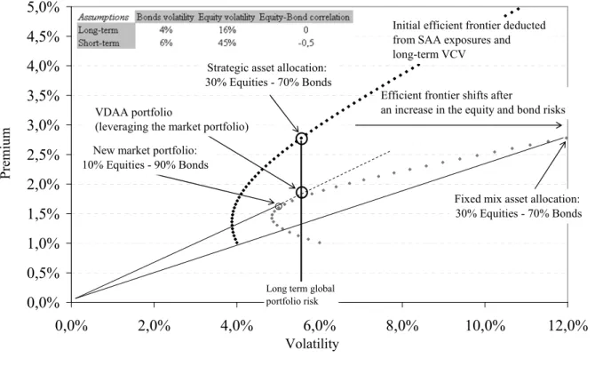
The algorithm is thus a pure risk adjustment procedure, keeping constant expected returns and translating the initial allocation in the new risk context. This fully invested portfolio is then diluted or leveraged with cash in order to match the original level of global portfolio volatility. Exhibit 1 shows an illustration of the procedure applied to a two-asset portfolio.

- Insert Exhibit 1 here -

In this example, the risk and expected returns define the strategic efficient frontier. After a market shock, equity volatility increases as does bond risk, and the correlation becomes negative (flight to quality). The frontier is both translated and deformed, with the new optimal portfolio being titled towards bonds. This portfolio is then leveraged if necessary ie if it displays a risk level inferior to the strategic volatility target. As we have seen, the adjusted

allocation results solely from the modification of the variance-covariance matrix. This dynamic portfolio now constitutes the new benchmark with which the currently held portfolio is compared upon which the latter will be rebalanced.

If the rebalancing is associated with high transaction costs (which might be the case when implementing the portfolio adjustments through cash products rather than derivative instruments), several methods can be used to determine its timing. For instance, portfolio adjustments are implemented if and only if the ex-ante tracking error of the current portfolio against the dynamic SAA exceeds a certain threshold; otherwise the weight drifts are not deemed significant enough and the portfolio is left untouched. Alternatively, a statistical approach can be used to determine when the new weights of the benchmark change significantly, as opposed to the normal estimation noise.

Intuitively, the effectiveness of the procedure depends crucially on the existence of regimes or persistence in volatility since, if it was not the case, the short term VCV matrix would yield no additional information but instead pure estimation noise over the long term VCV matrix.

IMPLEMENTATION AND BACK-TESTING

Given an initial strategic allocation, the only inputs required are the unconditional (i.e. long-term) and conditional (i.e. short-long-term) covariance matrices. The long-term variance-covariance matrix is estimated from historical data using a window consistent with the horizon of the strategic investment (typically between 5 and 20 years). Depending on the number of assets classes in the allocation, a shrinkage method can be used to stabilize the matrix with some structural prior (such as a zero correlations matrix, for instance).

Concerning the short-term VCV matrix, we have specified a fixed length for the window of estimation since we are interested not only in the accuracy of the estimate but also in the stability of the optimized weights in the portfolios. On a typical portfolio of half a dozen asset

classes and using daily observations, we found by means of trial and error that nine months was the optimal window length, because longer samples are not reactive enough while smaller ones are too noisy. We also used a filter to reduce the estimation noise on correlations and to stabilize the VCV matrix exploiting a clustering method as econophysics literature (Tola and al. [2008]) has shown that these techniques for building variance-minimizing portfolios are roughly as effective as more complex or data-intensive models. Obviously this doesn’t preclude the use of forecasting models if some are found to be more advantageous.We thus end up with two measurements of risk at each point in time, one over the long-term using all available data and a short-term one with a much shorter horizon reflecting current conditions. We have built a simple case study with two assets -equities and bonds -respectively expressed through the S&P500 and JPM US Government bond benchmarks, both in USD.

- Insert Exhibit 2 here -

Exhibit 2 displays the initial allocation (i.e. a SAA with 25% equities and 75% bonds) together with the strategic parameters derived from it. It appears that for such SAA – and based on the 1992-2010 historical period – almost two-third of the total portfolio risk comes from equity.

- Insert Exhibit 3 here -

Exhibit 3 shows the evolution of the weights according to the algorithm keeping the ex-ante volatility of the portfolio constant whenever possible. In this simple case, short-selling is not authorized meaning that it is not possible to borrow cash to invest in risky assets (in this long-only case, the dynamic portfolio’s ex- ante volatility might be lower than its target in certain circumstances – notably after an increase in asset volatility). Although not a strategic component of the long term asset allocation, cash is nevertheless used to control the volatility of the portfolio in consistency with the portfolio separation theorem.

The algorithm is then benchmarked against two extremes rebalancing strategies: an allocation that is rebalanced regularly (e.g. monthly) on its strategic weights (fixed mix strategy), and an allocation that is never rebalanced and whose exposures vary with the performances (a phenomenon known as equity drift or buy-and-hold approach).

- Insert Exhibit 4 here -

Exhibit 4 shows the performances of the three allocations through the back-testing period. It appears that the relative performance of the different allocations depends on the prevailing equity momentum.

- Insert Exhibit 5 here -

The risk measures clearly show the interest of rebalancing, since the risk reduction is real, and the cost in terms of foregone performance is not obvious. The maximum drawdown of the VDAA algorithm occurs in 2000 (and ends in 2003) unlike the two others (with a peak in 2007). This effect is not only due to the dynamic control of the overall volatility, as a strategy which would simply dilute the fixed mix portfolio in cash to keep the volatility constant underperforms the VDAA (column “Fixed mixed with volatility controlled” of exhibit 5) with a higher Sharpe ratio compared to the fixed mix allocation (with a different scaling).

- Insert Exhibit 6 here -

Exhibit 6 shows the ex-ante volatilities of each allocation at any point in time in order to make the process more explicit. The unconditional volatility is updated with the new observations and is subject to changes even with 20 years of data, meaning the same strategic allocation will correspond to different arbitrage opportunities depending on the moment of its inception.

ROBUSTNESS STUDY

Some implementation issues have been discovered in practice. First, as mentioned above, the unconditional volatilities and correlations are subject to changes and can thus induce some instability in output weights. A possible solution is to resort to a suitable prior for shrinkage. Secondly, as the risk of a balanced portfolio is overwhelmingly driven by equity risk, the contributions of low-risk assets in such a portfolio have little elasticity to the weights in these assets. Therefore the optimization can yield different weights on these assets for the same risk breakdown and thus different optimal exposures for the other assets. In order to avoid unnecessary transactions, a solution would be to penalize turnover in the optimization or to determine statistically significant deviation from the current weights. Thirdly, the main issue is the robustness of the backtest results. Clearly the historical backtest is of limited use, since the reduction in equity exposure is justified ex-post by the stalling of equity indexes over the last ten years. In order to get a better insight into the workings of the procedure, we need to build hypothetical scenarios that retain the characteristics of the asset price without reproducing the exact historical path.

To make sense, any robustness study should reflect reality as closely as possible. Simulated paths should reproduce both the unpredictability of returns (Merton [1980]) and the persistence in volatility dynamics. Our scenarios are built with the only assumption that volatility exhibits long memory (Banerjee and Urga [2005]). Indeed this fundamental property is what justifies the algorithm: even though the volatility is stationary over the long term, it passes through regimes lasting long enough that it becomes valuable to adjust the allocation. To reproduce this stylized fact, we use the stationary bootstrap of Politis and Romano [1999] with the additional restriction that the new bootstrapped blocks have to be taken in the temporal neighbourhood of the last draw, thus insuring that regimes are preserved with occasional abrupt shifts. The simulations consist in producing counter-factual histories of

asset prices and then applying the rebalancing algorithm to them, in order to uncover the distributions of the portfolio characteristics. The initial strategic portfolio exposures are to be picked at random in order to cover the most various views.

- Insert Exhibits 7 and 8 here -

Exhibit 7 shows for each simulation the Sharpe ratio of fixed-mix and VDAA strategies as compared to the naïve buy-and-hold allocation. Exhibit 8 reveals that rebalancing on fixed weights proves better than not doing so in all cases. Rebalancing on our dynamic benchmark looks equivalent to using fixed weights when returns are high, but is better in the least favourable cases.

This robustness study confirms the initial backtest results: the VDAA algorithm dominates both buy-and-hold and fixed mix in terms of remuneration of the risk taken. The VDAA algorithm, which produces the highest ex-ante Sharpe ratio overall, also delivers the highest ex-post Sharpe ratio within our simulation framework. These results are a joint test of both the validity of the procedure and the accuracy of the underlying hypothesis on the volatility dynamics. They do not (and cannot) prove the superiority of the algorithm for all situations; they merely confirm that if the regime shifts are a good description of the reality then this process is appropriate, and its implementation does not destroy the theoretical value.

CONCLUSION

Commitment to a rebalancing strategy requires absolute clarity about the investor objective because there is a trade-off between risk and return that ultimately depends on the investor’s risk aversion. When risk perception spikes, the increase in return might not be sufficient to compensate for greater volatility, meaning that the portfolio Sharpe ratio deteriorates. Our VDAA approach offers a disciplined solution for portfolio rebalancing consistent with this trade-off, in order to maintain the maximum Sharpe ratio at all times.

For some investors, the asset management industry has failed in implementing active asset allocation decisions, especially during recent years. This may be attributable to the fact that most of the investment processes have attempted to merge two different objectives at once: simultaneously controlling the risk and creating alpha. As there are two different purposes that can not be merged, it makes sense to have two different processes and to split the risk budget in two parts, each of them with its own investment process. The aim of the volatility-driven asset allocation is not to generate alpha but simply to adapt the strategic allocation of the investor to changes in the risk environment, answering so to the first need, controlling the risk. Results so far indicate that this solution delivers the intended result, providing a tighter risk control and allowing the investor to separate effectively tactical decisions and strategic hedging. But our VDAA methodology is not enough by itself and it is necessary to complete this risk-controlled process with an opportunistic tactical one.

E

1

Illustration of the procedure with an equity-bonds portfolio

0,0% 0,5% 1,0% 1,5% 2,0% 2,5% 3,0% 3,5% 4,0% 4,5% 5,0% 0,0% 2,0% 4,0% 6,0% 8,0% 10,0% 12,0% Volatility Premiu m

Strategic asset allocation: 30% Equities - 70% Bonds

New market portfolio: 10% Equities - 90% Bonds

Efficient frontier shifts after

an increase in the equity and bond risks

Fixed mix asset allocation: 30% Equities - 70% Bonds Initial efficient frontier deducted from SAA exposures and long-term VCV

Long term global portfolio risk

VDAA portfolio

(leveraging the market portfolio)

E

2

Strategic Asset Allocation (1992-2010)

S&P 500 JPM Government

Bonds Global portfolio

Weights 25% 75% 100%

Risk Contributions 3.5% 1.9% 5.4%

E

3

Evolution of the VDAA exposures (1992-2010)

0% 10% 20% 30% 40% 50% 60% 70% 80% 90% 100% 1992 1994 1996 1998 2000 2002 2004 2006 2008 E xposure s

Equities Bonds Cash

E

4

Performance of the rebalancing algorithm

100 150 200 250 300 350 1992 1994 1996 1998 2000 2002 2004 2006 2008

Buy-and-hold Fixed Mix VDAA

E

5

Characteristics of the three different rebalanced portfolio

Buy-and- hold

Fixed Mix Fixed Mix with Volatility- controlled VDAA Return 6.7% 6.8% 6.5% 7.1% Volatility 6.5% 5.4% 4.9% 4.9% Sharpe Ratio 0.65 0.82 0.83 0.95 Max. Drawdown 13.2% 10.6% 9.2% 7.8%

Peak 06-dec-07 06-dec-07 06-dec-07 01-sep-00

Valley 09-mar-09 09-mar-09 27-oct-08 23-jul-02

End 11-mar-10 10-sep-09 16-mar-10 17-apr-03

E

6

Ex Ante Volatilities of the allocations

2% 4% 6% 8% 10% 12% 14% 1992 1994 1996 1998 2000 2002 2004 2006 2008

E

7

Sharpe ratios of fixed mix and volatility driven allocations function of the buy-and-hold Sharpe ratio -0,25 0,00 0,25 0,50 0,75 1,00 1,25 1,50 1,75 2,00 2,25 2,50 -0,25 0,00 0,25 0,50 0,75 1,00 1,25 1,50 1,75 2,00 2,25 2,50 Buy-and-hold Sharpe ratio

VDAA and

Fixed

M

ix Sharpe Ratios

Fixed Mix VDAA

E

8

Distribution of the characteristics of the process on simulated series

0% 10% 20% 30% 40% 50% 60% 70% 80% 90% 100% -0,25 0,00 0,25 0,50 0,75 1,00 1,25 1,50 1,75 2,00 2,25 2,50 Sharpe Ratio Cumulative Distribu tion

ENDNOTES

The authors would especially like to thank Heide Jimenez-Davila, Olivier Scaillet and Jérôme Teiletche for their helpful comments and suggestions.

REFERENCES

Banerjee, A., and G. Urga. “Modelling Structural Breaks, Long Memory and Stock Market Volatility: an Overview”, Journal of Econometrics, Vol. 129, No. 1 (2005), pp. 1-34.

Clark, P. “A Subordinated Stochastic Process Model with Finite Variance for Speculative Prices”, Econometrica, Vol. 41, No.1 (1973), pp. 135-156.

Diebold, F., and K. Yilmaz. “Macroeconomic Volatility and Stock Market Volatility, World-Wide”, NBER Working Paper, 2008.

Engle, R., E. Ghysels, and B. Sohn. “On the economic sources of stock market volatility”, Finance Working Paper, NY University, 2008.

Fleming, J., C. Kirby, and B. Ostdiek. “The Economic Value of Volatility Timing”, The

Journal of Finance, Vol. 56, No.1 (2001), pp. 329-352.

Fleming, J., C. Kirby, and B. Ostdiek. “The Economic Value of Volatility Timing Using Realized Volatility”, Journal of Financial Economics, Vol. 67, No. 3 (2003), pp. 473-509. Gomes, F. “Exploiting Short-Run Predictability”, Journal of Banking and Finance, Vol. 31, No. 5 (2003), pp. 1427-1440.

Kritzman, M., S. Myrgren, and S. Page. “Optimal rebalancing: a scalable solution”, Journal

of Investment Management, Vol. 7, No. 1 (2009), pp. 9-19.

Liu, J., F. Longstaff, and J. Pan. “Dynamic Asset Allocation with Event Risk”, Journal of

Finance, Vol. 58, No.1 (2003), pp. 231-259.

Lu, Y., and P. Perron. “Modeling and Forecasting Stock Return Using a Random Level Shift Model”, Journal of Empirical Finance, Vol. 17, No. 1 (2010), pp. 138-156.

Marquering, W., and M. Verbeek. “The Economic Value of Predicting Stock Index Returns and Volatility”, Journal of Financial and Quantitative Analysis, Vol. 39, No. 2 (2004), pp. 407-429.

Masters, S. “Rebalancing”, The Journal of Portfolio Management, Vol. 29, No. 3 (2003), pp. 52-57.

Merton, R. “An Intertemporal Capital Asset Pricing Model”, Econometrica, Vol. 41, No.5 (1973), pp. 867-887.

Merton, R. “On Estimating the Expected Return on the Market: An Exploratory Investigation”, Journal of Financial Economics, Vol. 8, No. 4 (1980), pp. 323-361.

Munnix M., R. Schäfer, and O. Grothe. “Estimating Correlation and Covariance Matrices by Weighting of Market Similarity”, Working Paper, arXiv:1006.5847v1, 2010.

Politis, D., J. Romano, and M. Wolf. “Subsampling”, New York: SpringerVerlag, 1999. Sun, W., F. Ayres, L. Chen, T. Schouwenaars, and M. Albota. “Optimal Rebalancing for Institutional Portfolios”, The Journal of Portfolio Management, Vol. 32, No.2 (2006), pp. 33-43

Tola, V., L. Fabrizio, M. Gallegati, and R. Mantenga. “Cluster Analysis for Portfolio Optimization”, Journal of Economic Dynamics and Control, Vol. 32, No. 1 (2008), pp. 235-258.

Disclaimer

The views and opinions expressed in this article are those of the authors and do not necessarily reflect the views and opinions of Lombard Odier Investment Managers.