Tidally-induced variations of pH at the head of the Laurentian Channel.

(1)

1

Tidally-induced variations of pH

1

at the head of the Laurentian Channel

2 3

Alfonso Mucci1_{, Maurice Levasseur}2_{, Yves Gratton}3_{, Chloé Martias}1_{, Michael Scarratt}4_, 4

Denis Gilbert4, Jean-Éric Tremblay2, Gustavo Ferreyra5 and Bruno Lansard6 5

1- GEOTOP and Department of Earth and Planetary Sciences, McGill University, 3450 6

University Street, Montréal, QC, Canada H3A 0E8 7

2- Québec-Océan and Département de Biologie, Université Laval, 1045 Avenue de la 8

Médecine, Québec, QC, Canada G1V 2R3 9

3- Institut national de la Recherche Scientifique, Eau Terre et Environnement, 490 rue de la 10

Couronne, Québec, QC, Canada G1K 9A9 11

4- Fisheries and Ocean Canada, Maurice Lamontagne Institute, 850 Route de la Mer, Mont-12

Joli, QC, Canada QC G5H 3Z4 13

5- Québec-Océans et Institut des Sciences de la Mer de Rimouski, 310 Allée des Ursulines, 14

Rimouski, QC, Canada G5L 3A1 15

6- Laboratoire des Sciences du Climat et de l’Environnement, avenue de la Terrasse, 16

domaine du CNRS, bât. 12, 91198, Gif-sur-Yvette, France 17

18

ABSTRACT 19

The head of the Laurentian Channel (LC) is a very dynamic region of exceptional 20

biological richness. To evaluate the impact of freshwater discharge, tidal mixing, and biological 21

activity on the pH of surface waters in this region, a suite of physical and chemical variables was 22

measured throughout the water column over two tidal cycles. The relative contributions to the 23

water column of the four source-water types that converge in this region were evaluated using an 24

optimum multi-parameter algorithm (OMP). Results of the OMP analysis were used to reconstruct 25

the water column properties assuming conservative mixing, and the difference between the model 26

properties and field measurements served to identify factors that control the pH of the surface 27

waters. These surface waters are generally undersaturated with respect to aragonite, mostly due to 28

Can. J. Fish. Aquat. Sci. Downloaded from www.nrcresearchpress.com by GOTEBORGS UNIV on 09/20/17

(2)

2 the intrusion of waters from the Upper St. Lawrence Estuary and the Saguenay Fjord. The presence 29

of a cold intermediate layer impedes the upwelling of the deeper, hypoxic, lower pH and aragonite-30

undersaturated waters of the Lower St. Lawrence Estuary to depths shallower than 50 meters. 31

32

RÉSUMÉ 33

La tête du chenal Laurentien est une région très dynamique d’une richesse biologique 34

exceptionnelle. Afin d’évaluer l’impact des apports en eaux douces, du mélange tidal, et de 35

l’activité biologique sur le pH des eaux de surface dans cette région, une suite de variables 36

physiques et chimiques a été mesurée dans la colonne d’eau sur deux cycles de marée. La 37

contribution relative des quatre sources d’eau-type qui convergent dans cette région a été évaluée 38

à l’aide d’un algorithme d’optimisation multi-paramétrique (OMP). Les résultats de l’OMP ont été 39

utilisés pour reconstruire les propriétés de la colonne d’eau en assumant un mélange conservateur 40

et la différence entre les propriétés issues du modèle et des mesures effectuées sur le terrain ont 41

servies à identifier les facteurs qui contrôlent le pH des eaux de surface. Les eaux de surface sont 42

généralement sous-saturées par rapport à l’aragonite, surtout à cause de l’intrusion d’eau provenant 43

de l’estuaire fluvial du Saint-Laurent et du fjord du Saguenay. La présence de la couche 44

intermédiaire froide (CIF) durant les marées de morte-eau tamponne l’acidification des eaux de 45

surface dans cette région de l’estuaire. La présence d’une couche intermédiaire froide limite la 46

remontée des eaux profondes, hypoxiques, de faible pH et sous-saturées par rapport à l’aragonite 47

de l’estuaire maritime du Saint-Laurent à des profondeurs de moins de 50 mètres. 48

49

50

(3)

3 INTRODUCTION

51

The oceans have absorbed approximately 30% of the anthropogenic CO2 released to the 52

atmosphere since the beginning of the industrial revolution (Sabine et al. 2004). Consequently, 53

over the last century, the pH of the global ocean surface has decreased by an estimated 0.1 unit, 54

equivalent to a 30% increase in the proton concentration (Caldeira and Wickett 2005). The 55

increased acidity has lowered the saturation state of ocean waters with respect to calcite and 56

aragonite (the two most common CaCO3 polymorphs that constitute the shells and skeleton of 57

many marine organisms) and, in combination with other stresses such as global warming, likely 58

affected the ecology of carbonate-secreting organisms (Fabry et al. 2008, Miller et al. 2009; Ries 59

et al. 2009; Kroeker et al. 2013) as well as non-calcifiers because pH plays a critical role in 60

mediating many physiological processes (Fabry et al. 2008; Kroeker et al. 2013). 61

The pH of surface waters in coastal systems is controlled by more dynamic processes than 62

in the open ocean. In these systems, the pH of surface waters may exhibit important short (hours) 63

and long (season) term variations in response to freshwater inputs and vertical mixing (Abril et al. 64

2000; Feely et al. 2010). Freshwater rivers and inner estuaries are typically supersaturated in CO2 65

with respect to the atmosphere (Meybeck 1993; Raymond et al. 1997; Barth et al. 1999; Bauer et 66

al. 2013; Dinauer and Mucci 2017) as a result of inputs from their drainage basin and the activity 67

of heterotrophic organisms sustained by natural or anthropogenic terrestrial and riverine organic 68

carbon inputs (Frankinouille et al. 1996, 1998; Feely et al. 2010). Consequently, waters are often 69

characterized by circum-neutral to slightly acidic pHs (Wallace et al. 2014) and are a net source 70

of CO2 to the atmosphere (see compilation in Chen and Borges 2009). The high primary 71

productivity characterizing estuarine systems, in combination with their deep-water circulation, 72

favor the accumulation of respiratory CO2 at depth in stratified estuaries and a further decrease in 73

(4)

4 pH (Taguchi et al. 2010; Cai et al. 2011; Mucci et al. 2011, Wallace et al. 2014; Hagens et al. 74

2015). In urbanized areas, this phenomenon can be exacerbated by eutrophication (Borges and 75

Gypens 2010; Sunda and Cai 2012; Melzner et al. 2013). Since variations in pH in coastal waters 76

are typically recurrent and of greater amplitude than those observed in the open ocean, one could 77

surmise that the estuarine biota will be more resilient to pH fluctuations than open ocean biota. In 78

order to evaluate the risk posed by ocean acidification on marine organisms in coastal systems, it 79

is thus essential to know the chemical properties of source waters, the relative contribution of each 80

to the coastal waters and their temporal variations. This knowledge is also required in order to 81

develop realistic experimental protocols to assess the sensitivity of estuarine organisms to ocean 82

acidification. 83

84

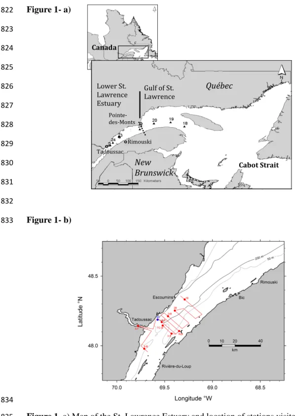
The head of the Laurentian Channel at the western limit of the Lower St. Lawrence Estuary 85

(LSLE, Figure 1) is one of the most dynamic regions of the St. Lawrence Estuary. Here, complex 86

tidal phenomena due to rapid shoaling (tidal movements, including internal tides and strong flows 87

over the steep entrance sill) generate significant mixing of near-surface waters with the deeper 88

saline waters, resulting in a nutrient-rich surface layer that sustains the feeding habitat of several 89

large marine mammals. Four different water masses converge at this location: the brackish surface 90

waters of the Upper St. Lawrence Estuary (USLE), the brackish surface waters discharged at the 91

mouth of the Saguenay Fjord, the cold intermediate layer (CIL) waters of the LSLE and the 92

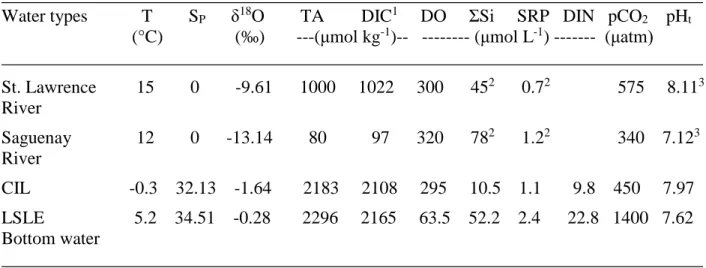
hypoxic bottom waters of the LSLE (Mucci et al. 2011). With the exception of the Saguenay River 93

waters, the other water masses are supersaturated in CO2 with respect to the atmosphere (Table 1), 94

the supersaturation having been acquired from their tributaries and/or the accumulation of 95

metabolic CO2 from microbial respiration of autochtonous or allochthonous organic matter (Yang 96

(5)

5 et al. 1996; Barth et al. 1999; Wang and Veizer 2000). The objective of this study was to assess 97

how the confluence and mixing of these different water masses affect the chemical and biological 98

properties of the surface waters over two tidal cycles at a fixed station at the head of the Laurentian 99

Channel. After identifying the properties of the individual end-member water-mass types, we 100

estimated the relative contribution of each water-mass type to the surface waters at the fixed station 101

by solving for a set of linear equations for conservative and non-conservative properties. A 102

reconstruction of the water column properties at the fixed station and a comparison with field 103

measurements are used to identify factors that control the pH of surface waters in this region over 104

the study period. 105

106

Study Site:

107

The St. Lawrence Estuary

108

The St. Lawrence Estuary (SLE) receives the second largest freshwater discharge (11900 m3 109

s-1) in North America (El-Sabh and Silverberg 1990). It begins at the landward limit of the salt 110

intrusion near Ile d’Orléans and extends 400 km seaward to Pointe-des-Monts and the Gulf of St. 111

Lawrence (GSL), a semi-enclosed sea connected to the Atlantic Ocean via Cabot Strait and the 112

Strait of Belle-Isle (Fig. 1). The Upper St. Lawrence Estuary (USLE) is the relatively shallow, well 113

mixed, and fully oxygenated transition zone between the mouth of the St. Lawrence River at 114

Quebec City and the marine region (SP≈ 25 and greater) beginning at Tadoussac (Fig. 1). At the 115

transition between the Upper and Lower St. Lawrence Estuary, the water column deepens from 50 116

m to 300 m over less than 20 km, in an area characterized by diverse and complex tidal phenomena 117

(Gratton et al. 1988; Saucier and Chassé 2000). The dominant bathymetric feature of the Lower 118

St. Lawrence Estuary (LSLE) is the Laurentian Channel, a 1240 km long, 250-500 m deep 119

(6)

6 submarine valley that extends from the edge of the eastern Canadian continental shelf, through 120

Cabot Strait, to the confluence of the St. Lawrence Estuary and the Saguenay Fjord at Tadoussac. 121

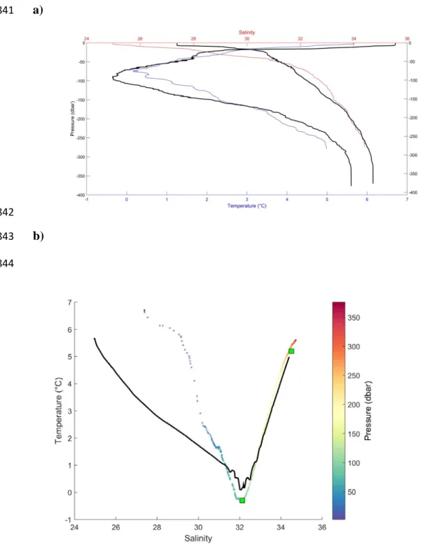
The water column in the LSLE is strongly stratified and, throughout most of the year, is 122

characterized by three distinct layers (Dickie and Trites 1983): (1) a thin surface layer (25-50 m 123

deep) of low salinity (27-32) flowing seaward, (2) an intermediate cold (-1 to 2°C) and saline 124

(31.5-33) layer (CIL) that originates in the Gulf in the winter, extends to about 150 m depth, and 125

flows landward, and (3) a warmer (4-6°C) and saltier (34-34.6) deep layer (150+ m) that flows 126

landward (El-Sabh and Silverberg 1990). Two typical vertical profiles taken at one of our sampling 127

stations, station 1B (Figure 1b: 48°19.8’N, 069°17.4’W; June 11, 2013; 16:48GMT) and at station 128

18 (Figure 1a: 49° 16.0, 064° 16.5; June 7, 2013; 16:01 GMT) are reproduced in Figure 2. The 129

surface layer displays large seasonal variations in temperature and salinity due to atmospheric and 130

buoyancy (i.e., runoff events) forcing. In winter, the surface layer becomes progressively colder 131

and denser, as tributary flow decreases, air temperatures plummet, and ice forms, until it merges 132

with the intermediate layer (Gilbert and Pettigrew 1997; Galbraith 2006). The deep waters are a 133

mixture of Labrador Current and North Atlantic Central waters whose proportions vary on a 134

decadal or secular timescale (Bugden 1991; Gilbert et al. 2005). The transit time of a parcel of 135

water between the seaward end of the Laurentian Channel at the edge of the continental shelf and 136

the head of the Channel at Tadoussac has been estimated at 4 to 7 years (Bugden 1991, Gilbert 137

2004) whereas the mean age of the deep waters of the LSLE is believed to be ~20 years (Mucci et 138

al. 2011). Given the properties of the source waters, benthic and pelagic respiration along the 139

Channel, and their mean age, the bottom waters of the LSLE are hypoxic (<20% oxygen saturation; 140

Gilbert et al. 2005), charged with metabolic CO2 and therefore acidified (Mucci et al. 2011). The 141

landward end of the Laurentian Channel marks the transition from the Lower to the Upper St. 142

(7)

7 Lawrence Estuary, the mouth of the Saguenay Fjord, and the marine region (SP≈ 25 and greater) 143

beginning at Tadoussac (Fig. 1). Typical semi-diurnal (M2) tidal current amplitudes in the LSLE 144

are on the order of 0.2 m s-1 (Saucier and Chassé 2000), so that tidal excursions are on the order 145

of 3 km. 146

The Saguenay Fjord

147

The Saguenay Fjord is a 93 km long, 1-6 km wide and 275 m deep U-shaped submerged 148

valley, bounded by sheer, vertical walls that reach up more than 300 m above the water line. 149

Situated approximately 150 km northeast of Quebec City on the north shore of the St. Lawrence 150

Estuary, it connects with the estuary at Tadoussac through a 20-m deep sill. Its bathymetry is 151

defined by three basins separated by two sills at 60 and 120 m depth, located approximately 20 km 152

and 30 km, respectively, from the mouth of the fjord. A short account of its geological history and 153

physiographic features can be found in Schafer et al. (1990) and Locat and Levesque (2009). 154

The water column of the Saguenay Fjord is characterized by a sharp pycnocline that 155

separates two distinct water masses. The thick bottom layer is well-mixed and oxygenated, with 156

waters penetrating landward from the St. Lawrence Estuary as they episodically spill over the sills 157

(Therriault and Lacroix 1977; Siebert et al. 1979; Stacey and Gratton 2001; Bélanger 2003; Belzile 158

et al. 2015). Bottom-water salinities are approximately 30.5 (Mucci et al. 2000), with temperatures 159

ranging from 0.4 to 1.7oC (Fortin and Pelletier 1995). The surface layer consists of brackish waters 160

(SP~0-10) resulting from the turbulent mixing of the outflow from the Saguenay River (and smaller 161

tributaries such as the Valin, Ha! Ha! and Mars Rivers) and the underlying marine waters. The 162

thickness of the surface layer, perhaps best defined by the depth of the 18.00 sigma-tee isopycnal, 163

typically increases towards the mouth of the fjord, but pinches off towards the surface at high tide 164

(8)

8 or when denser waters overspill the entrance sill. The surface water temperatures range from 165

freezing in winter to 16º_{C in summer (Fortin and Pelletier 1995). Detailed hydrographic} 166

characteristics of the fjord can be found in Schafer et al. (1990) and Gratton et al. (1994). 167

Figure 3 shows a 3-day average of sea-surface temperatures derived from satellite data 168

(OGSL 2014). A prominent tongue of cold surface waters due to upwelling and tidal mixing 169

extends from the head of the Laurentian Channel (near Tadoussac) to about Rimouski. Our fixed 170

station is located at the northern edge of this cold tongue. 171

Methods

172

Water column sampling

173

On June 10-15, 2013, we sampled the whole water column at six stations and surface waters 174

(3 – 5 m below the surface) at four stations along a saw-tooth transect at the head of the Lower St. 175

Lawrence Estuary (LSLE), the mouth of the Upper St. Lawrence Estuary (USLE) and the mouth 176

of the Saguenay Fjord (Figure 1). In addition, we sampled the whole water column every four 177

hours and surface waters (~3 m) every two hours over 50 hours at a fixed station (48°11.2’N, 178

69°34.4’W) a few kilometers east of the fjord’s mouth in the northern half of the head of the LSLE 179

in order to characterize changes in the properties of these surfaces waters over two tidal cycles. 180

Finally, the whole water column at four stations (Stations 23, 22, 20, 18) in the LSLE and western 181

Gulf of St. Lawrence was sampled on an earlier cruise (June 3-8, 2013) and these results served to 182

better define the properties of the source-water types encountered at the fixed station (see Water 183

mass analysis section below). Water samples were collected using a 12-Niskin bottle/CTD

184

(SeaBird SBE 911) rosette sampler onboard the R/V Coriolis II. Sampling depths were typically, 185

3, 10, 20, 40, 60, 80, 100, 150 m deep, in addition to 15 m above the bottom.The pH (on the NBS 186

(9)

9 scale - pHNBS), dissolved oxygen (DO), temperature and conductivity probes were calibrated by 187

the manufacturer during the winter months preceding the cruise. Nevertheless, discrete samples 188

were taken from the Niskin bottles for laboratory measurements of pH (total proton concentration 189

scale – pHT), DO and salinity and the CTD records re-calibrated post-cruise. Additional surface 190

water samples were collected, on distinct outings, in Chicoutimi (Saguenay River end-member) 191

and near Quebec City (St. Lawrence River end-member) during or within a week of the research 192 cruise. 193 194 Analytical methods 195

Discrete salinity samples taken throughout the water column were analyzed on a Guildline 196

Autosal 8400 salinometer calibrated with IAPSO standard seawater. The instrument has a 197

theoretical accuracy < ± 0.002. Dissolved oxygen (DO) concentrations were determined by 198

Winkler titration (Grasshoff et al. 1999) of water samples recovered from the Niskin bottles. The 199

relative standard deviation, based on replicate analyses of samples recovered from the same Niskin 200

bottle, was better than 1%. These measurements further served to calibrate the SBE-43 oxygen 201

probe mounted on the rosette. 202

Water samples destined for pH and titration alkalinity (TA) measurements were transferred 203

directly from the Niskin bottles to, respectively, 125 mL plastic bottles without headspace and 250 204

mL glass bottles, as soon as the rosette was secured onboard. In the latter case, a few crystals of 205

HgCl2 were added before the bottle was sealed with a ground-glass stopper and Apiezon® Type-206

M high-vacuum grease. 207

(10)

10 The pH of the 125 mL samples was determined onboard using a Hewlett-Packard UV-208

Visible diode array spectrophotometer (HP-8453A) and a 5-cm quartz cell after thermal 209

equilibration of the sampling bottles in a constant temperature bath at 25.0±0.1°C. Phenol red 210

(PR; Robert-Baldo et al. 1985) and m-cresol purple (mCP; Clayton and Byrne 1993) were used as 211

indicators. The absorbance at the wavelengths of maximum absorbance of the protonated (HL) 212

and deprotonated (L) indicators were measured and recorded. A similar procedure was carried out 213

several times each day using TRIS buffers prepared at practical salinities (SP) of ~35 and ~25 214

(Millero 1986). The pH on the total proton concentration scale (pHT) of the samples and buffer 215

solutions were calculated according the equation of Byrne (1987). The salinity-dependence of the 216

dissociation constants and molar absorptivities of the indicators were taken from Robert-Baldo et 217

al. (1985) for phenol red and from Clayton and Byrne (1993) for m-cresol purple. The salinity-218

dependence of the phenol red indicator dissociation constant and molar absorptivities was 219

extended (from SP = 5 to 35; Bellis 2002) to encompass the range of salinities encountered in this 220

study, but computed pHTs from the revised fit were not significantly different from those obtained 221

with the relationship provided by Robert-Baldo et al. (1985). All measurements were converted to 222

the total proton scale using the salinity of each sample and the HSO4- association constants given 223

by Dickson (1990). Reproducibility and accuracy of our TRIS buffer measurements were on the 224

order of 0.005 pH units or better. The computed pHTs at 25°C and 1 atmosphere total pressure 225

were then used in combination with the measured TA to calculate the pHTs at the in-situ 226

temperature and pressure using the Microsoft Excel version of CO2SYS (Pierrot et al. 2006), based 227

on the original algorithm of Lewis and Wallace (1998), and the carbonic acid dissociation 228

constants of Cai and Wang (1998), the total boron concentration [B]T value from Uppström (1974), 229

and the standard acidity constant of the HSO4- ion (K(HSO4)) from Dickson (1990). 230

(11)

11 The titration alkalinity (TA) was determined at the land-based laboratory within one week 231

of sampling by open-cell automated potentiometric titration (Titrilab 865, Radiometer®_{) with a pH} 232

combination electrode (pHC2001, Red Rod®) and a dilute (~0.025N) HCl titrant. The latter was 233

calibrated against Certified Reference Materials (CRM Batch#94, provided by A. G. Dickson, 234

Scripps Institute of Oceanography, La Jolla, USA). Samples were drawn from the 250 mL sample 235

bottle and weighed on an analytical balance to ± 0.1 mg. The average relative error, based on the 236

average relative standard deviation on replicate standard and sample analyses, was better than 237 0.15%. 238 239 Nutrients 240

Subsamples for nutrient determinations were filtered through a 0.45 µm disposable syringe 241

filter to remove particles. Dissolved NH4+ concentrations were determined immediately onboard 242

with the fluorometric method described by Holmes et al. (1999), with a detection limit of 0.01 µM. 243

For nitrate, nitrite, soluble reactive phosphorus (SRP) and soluble reactive silicon (SRS), filtered 244

samples were collected into acid-washed 15-ml polyethylene tubes and quickly frozen and stored 245

at -20°C. Back at home laboratory, frozen samples were rapidly thawed and concentrations of 246

inorganic nutrients were determined using the routine colorimetric method adapted from Hansen 247

and Koroleff (2007) with a Bran and Luebbe Autoanalyzer III. The analytical detection limit was 248

0.02 µM for nitrite, 0.04 µM for nitrate+nitrite (hereafter dissolved inorganic nitrogen, DIN), 0.05 249

µM for SRP and 0.1 µM for silicate. 250

251

(12)

12

Isotopic composition

252

Water samples for isotopic analysis were collected in 13 mL screw-top plastic test tubes. 253

The stable oxygen isotopic composition (δ18O) of the water samples was analyzed at the GEOTOP-254

UQAM stable isotope laboratory. 200-μL aliquots of the water samples and two laboratory internal 255

reference waters were transferred into 3-mL vials stoppered with a septum cap. The vials were 256

then placed in a heated rack maintained at 40°C. Commercially available CO2 gas was introduced 257

in all the vials using a Micromass AquaPrep and allowed to equilibrate for 7 hours. The headspace 258

CO2 was then sampled by the Micromass AquaPrep, dried on a -80°C water trap, and analyzed on 259

a Micromass Isoprime universal triple collector isotope ratio mass spectrometer in dual inlet mode. 260

Data were normalized against the two internal reference waters, both calibrated against V-SMOW 261

and V-SLAP. Data are expressed in ‰ with respect to V-SMOW, and the average relative standard 262

deviation on replicate measurements of sample waters is better than 0.05‰. 263

264

Water mass analysis

265

The water mass analysis was performed using the optimum multi-parameter algorithm 266

(OMP) of Karsteen and Tomczak (1999), originally developed by Tomczak (1981). OMP analysis 267

is based on a simple model of linear mixing. It assumes that all water mass properties undergo the 268

same mixing process, i.e. their mixing coefficients are identical, as is the case in turbulent mixing. 269

The spatial water mass distribution can therefore be determined through a linear set of mixing 270

equations. OMP determines the contributions of pre-defined end-member water masses (so called 271

source-water types or SWT) to a sample. The SWT contributions or fractions (Xi) for each data 272

point are obtained by finding the best linear mixing combination in parameter space defined by 273

temperature, salinity, oxygen, total alkalinity and δ18O which minimizes the residuals in a non-274

(13)

13 negative least squares analysis. The solution includes two physically realistic constraints: (i) the 275

contributions from all sources must add up to 100%, and (ii) all contributions have to be non-276

negative. 277

Based on the description of the water circulation in the LSLE, four different source-water 278

types contribute to the water column properties at the head of the Laurentian Channel: the 279

freshwaters of the St. Lawrence and Saguenay Rivers, the saline and cold intermediate layer water 280

and the upwelling saline hypoxic bottom water of the LSLE. Even though the properties of the 281

source-water types are variable in both space and time, we use the dataset acquired during this 282

study as well as data acquired a week before on another cruise along a seaward transect through 283

the Lower Estuary and Gulf of St. Lawrence to define the most representative properties for each 284

source-water type (Table 1). This allows the direct comparison of the water mass fractions and 285

their vertical distribution at the time of sampling. Whereas OMP analysis was initially used to 286

distinguish and calculate the relative contributions of each source-water type in a parcel of water 287

using temperature, practical salinity (SP) and nutrient data (Mackas et al. 1987), in this study, we 288

used SP, the titration alkalinity (TA), and δ18O(H2O) as conservative tracers as well as temperature 289

and dissolved O2 (DO) concentrations as non-conservative tracers, to constrain the water mass 290

analysis. Non-conservative tracers should be applied with caution in OMP, because of temporal 291

and spatial variability, particularly in the surface waters. For example, the temperature of the 292

Saguenay River water ranges from 0°C in winter to +16°C in summer whereas the temperature of 293

the St. Lawrence River ranges from 0°C in winter to >20°C in summer. Dissolved O2 concentration 294

was also used as a non-conservative tracer, because it is a function of temperature (e.g. O2 295

solubility increases with decreasing temperature and salinity) and, like ΣSi and SRP, also a 296

function of primary production and biological respiration. Consequently, end-member matrix and 297

(14)

14 sample observations were multiplied by a diagonal weight matrix to account for differences in 298

tracer reliability, environmental variability, and precision of the data (Table 2). The error 299

associated with the water mass fraction analysis was estimated to be about ±10% of the fractional 300

values (Macdonald et al. 1989; Lansard et al. 2012). 301

302

Results and discussion

303

Variations of the water properties over two tidal cycles

304 305

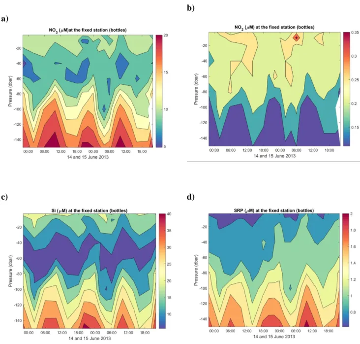
Figures 4a-l show time-series of water property profiles from the CTD (1-m resolution) at 306

the fixed station (SF) over two tidal cycles from June 13 to June 15, 2013. Results of the OMP 307

analysis are presented in Figures 5a-d. 308

The tides are very strong in the fixed station region. The impact of tides on the local 309

circulation is described in detail in Saucier and Chassé (2000). Near the SF, the tidal elevation in 310

the channel can be larger than 5 m (unpublished data) at the spring tide. Mertz and Gratton (1990) 311

reported internal oscillations on the order of 40-60 m over a tidal semi-diurnal cycle. Similar 312

oscillations can be observed on Figures 4a,b,c. The cold, upwelled water can reach the surface and 313

be observed flowing downstream as on Figure 3. As observed on this figure, our SF is located at 314

the edge of these cold surface waters. 315

Surface salinities decrease and temperatures increase during ebb tide (Figs. 4a,b), as 316

freshwaters from the Saguenay and the St. Lawrence Rivers, but mostly of the latter (Figs. 5a,b), 317

intrude into the Lower St. Lawrence Estuary (LSLE) and at our fixed station. The intrusion is 318

detectable to depths of about 30 m and accompanied by a slight (less than 0.1 pH unit) decrease in 319

pH (Fig. 4f). Higher salinity, lower temperature and higher pH waters impinge closer to the surface 320

(15)

15 during the flood tide whereas patches of low pH waters from the Saguenay Fjord persist at the 321

surface well into flood tide (Figs. 4a,b,f). The former correspond to the upwelling/invasion of the 322

cold intermediate layer (CIL) nearly up to the surface where it accounts for more than 80% of the 323

mixture (Fig. 5c). Temporal variations of the surface-water titration alkalinity (TA) and dissolved 324

inorganic carbon (DIC) concentrations are almost perfectly correlated with those of the salinity 325

(Figs. 4e,g). Temporal variations of the surface-water major nutrient concentrations are more 326

diffuse, but are nonetheless either correlated (SRP (r2_{= 0.63); Fig. S1) or anti-correlated (DIN (r}2 327

= 0.46) and ΣSi (r2 = 0.62); Fig. S1) to salinity in the top 3 m, reflecting the differential input from 328

the freshwaters (Saguenay and St. Lawrence Rivers) and the CIL. 329

Irrespective of the tide, dissolved oxygen concentrations remain high (> 260 µM, Fig. 4d) 330

throughout the top 80-100 m of the water column. Likewise, the computed pCO2 in the top 80 m 331

of the water column is slightly supersaturated with respect to the atmosphere (~ 400 µatm) and 332

shows few discernible features, except for a greater pCO2 supersaturation at low tide when the 333

contribution of freshwaters from the St. Lawrence River and Saguenay Fjord, both of which are 334

rich in metabolic CO2 and dissolved silicate (as well as ammonium in the latter case) relative to 335

the CIL, are maximum (Fig. 5a,b). 336

As expected, below 150 m depth, hypoxic bottom waters are dominated by Atlantic waters 337

that enter the Gulf and Estuary through Cabot Strait. These waters intrude to depths as shallow as 338

80 m at high tide (Fig. 5d). 339

340

pH in the surface waters

341 342

(16)

16 The pHT of the surface waters (top 3 m) varied from 7.855 to 7.934 during the 50-hour 343

survey, nearly as much as the world’s oceans have experienced as a result anthropogenic CO2 344

uptake over the last century (Caldeira and Wickett 2005). The pHT of surface waters is determined 345

by the relative contribution of the three source-water types (SLW, SRW, and CIL), itself 346

determined in great part by tidal mixing, as well as by gas exchange with the atmosphere, the 347

addition of metabolic CO2 through bacterial respiration and biological uptake of CO2 through 348

photosynthesis. Mucci et al. (2011) reported on the variation of surface-water (0-16 m depth 349

interval) pH over the period 1933-2009 (also limited to the ice-free season) in the Lower St. 350

Lawrence Estuary (LSLE). Unlike the deeper waters that have become hypoxic and acidified, the 351

pH of surface waters shows no systematic variations over this period. Although the intra-annual 352

variability reaches ~0.1 pH unit, the inter-annual variability is nearly null (slope = 0, p > 0.05; i.e., 353

no statistically significant temporal variation). Along the Estuary and Laurentian Channel, pH 354

variations can exceed the intra-annual variability in the LSLE as the salinity and balance between 355

respiration and photosynthetic rates vary (Dinauer and Mucci 2017). 356

357

Throughout the three-day survey, waters in the surface layer (0-3 m) at the sampling sites 358

were always supersaturated in CO2 (443-550 μatm) with respect to the atmosphere at the time of 359

sampling. The saturation state of the surface mixed layer water with respect to aragonite, given by: 360

ΩA = [Ca2+][CO32-]/K*A (1)

361

where K*A is the stoichiometric solubility of aragonite at the in-situ temperature and salinity and 362

1 atmosphere total pressure (Mucci, 1983), varied little during the sampling period and was close 363

to saturation (ΩA = 0.88 to 1.02, 0.95 ± 0.03, n=27, Fig. 6), but fell slightly below saturation (as 364

low as ΩA = 0.88) at low tide. Given the ratio of the stoichiometric solubility constants (K*A/K*C 365

(17)

17 = 1.5; Mucci, 1983), the saturation state of the surface waters with respect to calcite was close to 366

1.5. Deeper waters became undersaturated with respect to aragonite below 60-80 m reaching 367

saturations as low as 0.70, but remained supersaturated with respect to calcite to the bottom at the 368

fixed station. 369

370

Validation of the OMP analysis

371 372

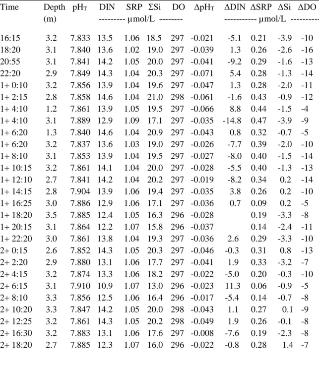
Using the results of the OMP analysis and the source-water type properties in Table 1, the 373

total alkalinity (TA), DIC and nutrient concentrations of each discrete water sample at the fixed 374

station was calculated, over the whole time series, assuming conservative mixing (i.e., closed 375

system). These computed values were then used as input parameters into CO2SYS to calculate the 376

pHT of the mixture and results compared to measured values. Differences between the calculated 377

and observed surface waters properties are compiled in Table 3; these reflect changes to the water 378

properties beyond those that can be accounted for by mixing of the source waters. The ΔpHcalc-379

meas values (thereafter referred to as ΔpHT) of the surface waters (1-3 m) are all negative (-0.004 380

to -0.066), indicating that either CO2 was lost by ventilation to the atmosphere or taken up by 381

photosynthesis during our observation period. As indicated above, surface waters remained 382

supersaturated with respect to the atmosphere throughout the sampling period and thus served as 383

a net source to the atmosphere. CO2 exchange across the air-sea interface is, however, a slow 384

process, much slower than for oxygen and most other gases (Zeebe and Wolf-Gladrow, 2001), 385

particularly under the low wind conditions (~5-28 knots) experienced during the cruise. Given 386

these wind speeds, the parameterizations of Raymond and Cole (2001) and Wanninkhof (2014) 387

for the gas transfer velocity, an average surface water pCO2 of 499 (± 26 μatm) during the sampling 388

(18)

18 period, and a local atmospheric pCO2 of 391 μatm, we estimated the air-sea CO2 efflux (loss of 389

CO2 to the atmosphere) to range between 2.6 and 4.8 mmol m-2 d-1. Over our sampling period, the 390

loss of CO2 to the atmosphere did not affect the DIC budget significantly (less than 1 μmol/kg) 391

and would have increased the surface-water pH by at most 0.003 unit, slightly below the 392

uncertainty of our field measurements. The positive ΔpCO2, ΔDIN and ΔSRP values (net DIC and 393

nutrient uptake) as well as negative ΔDO values (net oxygen production) in the surface waters are 394

clear evidence that photosynthesis (CO2 uptake, pH increase) dominated over respiration (CO2 395

production and pH decrease) and ventilation over the whole sampling period (Table 3). 396

Unfortunately, in the absence of independent estimates of the absolute photosynthetic and/or 397

respiration rates, we can only determine which of these two processes dominates. It is also 398

interesting to note that, despite the large uncertainties in the model and the intrinsic patchiness of 399

our measurements, the average ΔDIN:ΔSRP ratio (11 ± 4) nearly corresponds to the Redfield 400

stoichiometry of 15-16 (Redfield et al. 1963) and the DIN: SRP ratio (12, r2 = 0.79) below 30 m 401

depth in the LSLE. When the surface-water ΔpHT, ΔDIN, ΔSRP, ΔΣSi and ΔDO values are plotted 402

as function of the time of the day, no systematic variation with daylight is apparent (Fig. 7). The 403

study region is known to be an area of high primary productivity, notably during the spring tide 404

periods when upwelling and internal waves amplitude are maximum (Therriault and Levasseur 405

1985, Levasseur and Therriault 1987), but can be strongly suppressed spring fresh-water runoff 406

(Zakardjian et al. 2000). Hence, it is not surprising that we observe net autotrophy in the surface 407

waters but our conservative mixing model is not able to resolve the diurnal cycle of photosynthesis 408

and respiration, likely because it is not sensitive enough. Note that we have not modeled temporal 409

variations of pH below the surface mixed layer (SML) because, as shown in Figure 5, below ~30m, 410

the water column is entirely dominated by two water masses, the CIL between 30 and 50 m and 411

(19)

19 Atlantic (deep LSLE) waters below 150 m. In other words, with the exception of the SML, 412

significant variations in water column composition in response to the tide are only found between 413

50 and 150 m. Given that these waters are isolated from the atmosphere (no gas exchange), below 414

the euphotic zone (no photosynthesis), and respiration rates are negligible on the time scale of the 415

experiments, temporal variations are simply due to tidal oscillations. 416

417

Susceptibility of estuarine waters to acidification resulting from direct anthropogenic CO2 uptake 418

419

As noted above, most inner (river-dominated) estuaries are net sources of CO2 to the 420

atmosphere (Cai and Wang 1998; Chen and Borges 2009; Regnier et al. 2013). Their elevated DIC 421

enrichments and pCO2 supersaturations can mainly be attributed to the in situ microbial 422

degradation of internally and externally supplied organic carbon and the lateral transport of 423

inorganic carbon from rivers, coastal wetlands and ground waters (Bauer et al., 2013). Thus, these 424

waters do not directly take up anthropogenic CO2 from the atmosphere. Nonetheless, there have 425

been several reports of weak CO2 uptake by strongly stratified and/or marine-dominated (outer) 426

estuaries (Koné et al. 2009; Maher and Eyre 2012; Cotovicz Jr. et al. 2015), including the Lower 427

St. Lawrence Estuary (Dinauer and Mucci 2017). The resistance of these estuarine waters to a

428

decrease in pH in response to CO2 uptake is equated to a multiple of the carbonate ion

429

concentration ([CO32-]) (Stumm and Morgan 1996), and the latter, within the pH range of most of

430

these (7.5 < pHT <8.1), is approximated by TA – DIC (Broecker and Peng 1982).

431

Variations of the saturation state of waters with respect to aragonite (or calcite) depend

432

on the calcium and carbonate ion concentration product and the mineral solubility under in-situ

433

conditions (Eqn. 1). The [Ca2+] in estuarine waters is determined by the composition and mixing 434

(20)

20 ratio of the freshwater and seawater end-members, but given its high and conservative 435

concentration in seawater, the freshwater signature typically becomes indistinguishable (within a 436

1% deviation of the diluted seawater value) from that of seawater above a salinity of ~14. The 437

minimum salinity measured during our survey was 24.82. Hence, the [Ca2+] can accurately be 438

estimated from the measured salinities, i.e., [Ca2+] = SP * 0.01028/35 (Millero 2013). Both [Ca2+] 439

and K*A increase with salinity and to a similar extent (31% and 32.5%, respectively, over the range 440

of salinities encountered during our study), so that ΩA varies almost exactly with the [CO32-]. 441

Hence, again, the impact of CO2 uptake on the saturation state of most marine-dominated estuaries 442

is almost exclusively related to changes in [CO32-] which, as noted above, can be approximated by 443

(TA – DIC).

444 445

Biological response of some local CaCO3-secreting invertebrates to ocean acidification 446

447

Atmospheric CO2 uptake lowers the pH, the carbonate ion concentration and saturation 448

state of natural waters with respect to calcite and aragonite (ΩC and ΩA, respectively).

449

Consequently, the ability of many organisms to calcify is reduced by a decrease in the saturation

450

state of the waters and sediments they inhabit (Gazeau et al. 2013; Clements and Hunt 2017). 451

Aragonite being 50% more soluble than calcite (Mucci, 1981), organisms whose shells or skeletons 452

are partially or wholly aragonitic will be more susceptible to acidification. 453

Aragonite-undersaturated waters (ΩA < 1) dominate the top 20 metres of the water 454

column at the head of the Laurentian Channel except when the CIL intrudes almost up to the 455

surface at high tide. Below the CIL, the aragonite saturation depth (ΩA = 1) oscillates between 40 456

and 90 m reaching the shallowest depths at high tide when these waters are brought closer to the 457

(21)

21 surface. Hence, the recruitment, growth, metabolism and survival of calcifying invertebrates and 458

other benthic organisms exposed to these waters could be deleteriously affected (Parker et al. 2012; 459

Gazeau et al. 2010; Talmage et al. 2010; Kuhihara 2008). 460

Commercial harvesting of bivalve shellfish (scallops, soft-shell clams, mussels, Atlantic 461

surf-clams, Atlantic razor clams), echinoids (green sea urchin), and gastropods (common whelk) 462

in Quebec sustains several coastal communities with annual landings in the range of 2.5-4 million 463

dollars (DFO; http://www.qc.dfo-mpo.gc.ca/peches-fisheries/recreative-recreational/mollusque-464

mollusc-eng.asp?p=/peches-fisheries/recreative-recreational/mollusque-mollusc-eng.html). 465

Scallops (e.g., Chlamys islandica), soft-shell clams (e.g., Mya arenaria), the common whelk (e.g., 466

Buccinum undatum) and the green sea urchin (e.g., Stronylocentrotus droebachiensis) are found

467

on the seafloor near the head of the Laurentian Channel and, with the exception of scallops (Hutin 468

et al. 2005), are mostly harvested from no more than 20 m depth (Bernard Saint-Marie, DFO, pers. 469

comm.). Except for the green sea urchin, harvesting of the other species has declined steadily 470

since the beginning of the new millennium and there are currently no active commercial shellfish 471

fisheries in this region while recreational harvesting of scallops is now forbidden. The shells of 472

most bivalves and whelks found in the study area are composed of a combination of calcite and 473

aragonite (micro-) structural components (groups and layers) whereas the body and spines of sea 474

urchins are typically composed of high-magnesium calcite (more soluble than aragonite) and, thus, 475

their constant exposure to the aragonite-undersaturated (corrosive) waters in the top 20 m of the 476

water column and along the shorelines in the vicinity of the study area could possibly have 477

contributed, along with overfishing (Archambault and Goudreau 2006), to their decline. Since the 478

habitat of scallops extends to depths of 80 meters (the largest scallop bed in the vicinity of 479

Tadoussac is situated 5-10 km downstream of Ile Rouge in 40-80 m of water; Hutin et al. 2005), 480

(22)

22 this would put them well into the aragonite-undersaturated (corrosive) waters found below the 481

CIL. 482

To our knowledge, no specific study of the impacts of elevated pCO2s (lower pH and 483

ΩA) has been carried out on Chlamys islandica and Buccinum undatum, but studies conducted on 484

other species of scallops and whelk have reported deleterious effects on calcification and growth 485

of the former and the nutritional properties of the latter (Tate et al. 2017; Andersen et al. 2013). 486

Conversely, in addition to lowered calcification rates, the impacts of elevated pCO2 on Mya 487

arenaria were found to extend to their burrowing behavior, post-settlement dispersal (Clements et

488

al. 2016) as well as predator-prey interactions (Glaspie et al. 2017) whereas, in the case of 489

Stronylocentrotus droebachiensis, the effects extend to the fecundity, gonad growth, feeding rates

490

and susceptibility to metal toxicity (Lewis et al. 2016; Dupont et al. 2013; Siikavuopio et al. 2007). 491

Notwithstanding the potential impact of ocean acidification (OA) on the organisms 492

listed above, one should consider that these organisms may have, over time, developed a tolerance 493

or acclimatized to the high-amplitude and high-frequency (diurnal, seasonal) variations of 494

environmental variables (T, S, pH) encountered in dynamic estuaries such as the USLE, as has 495

been demonstrated in long-term exposures to elevated pCO2 (Dupont et al. 2013; Moulin et al. 496

2015; Uthicke et al. 2016). Whereas the above discussion is limited to commercially-harvested 497

CaCO3-secreting benthic organisms, OA may impact on the metabolic activity (e.g., survival, 498

growth, reproduction) of many other organisms, but an expanded discussion of these would be 499

well beyond the scope of this paper given the range of responses documented in the literature (e.g., 500

Doney et al. 2009). 501

502

(23)

23 In summary, the pH of surface waters at the head of the Laurentian Channel is modulated 503

by tides and mixing of three source–water types, the relatively high alkalinity (TA) and dissolved 504

inorganic carbon (DIC)-rich water of the St. Lawrence River (TA-DIC <0), the TA and DIC-poor 505

water of the Saguenay River (TA-DIC) <0) and saline waters of the TA and DIC-rich cold 506

intermediate layer (CIL) of the St. Lawrence Estuary (TA-DIC) >0) that upwell in this region. 507

Consequently, in-situ pHT values lower than 8.0 are found below the CIL or 80 m depth and in the 508

top 30 m of the water column. Nevertheless, upwelling of the TA-rich CIL and mixing with lower 509

salinity waters near the surface limit pH excursions within a narrow range (7.86 to 7.93) as the 510

(TA-DIC) of the mixture at our study site (head of the Laurentian Channel) was always positive. 511

The presence of the CIL also appears to impede the upwelling of the hypoxic, CO2-rich and 512

aragonite-undersaturated bottom waters of the Lower St. Lawrence Estuary (LSLE) to depths 513

shallower than about 80 m (Figure 5), although the large density gradient, as well as the tidal (~5 514

m) and internal-wave amplitudes (maximum 50-60 m), would not allow bottom waters to intrude 515

at the surface. The CIL is not unique to the SLE as similar layers are common in other subpolar 516

basins (Osafune and Yasuda 2006; Cyr et al. 2015). Organisms living within the first 20 meters of 517

the water column at the head of the Laurentian Channel are bathed, at low tide, by aragonite-518

undersaturated waters (ΩA < 1) intruding from the St. Lawrence and Saguenay Rivers. Likewise, 519

those that live below 80 meters depth, below the CIL, such as the largest scallop bed in the area, 520

are continuously exposed to the aragonite-undersaturated bottom waters (ΩA < 1) of the LSLE that 521

upwell up to nearly 40 metres from the surface at high tide. Whereas the growth, recruitment, and 522

other metabolic functions of CaCO3-secreting invertebrates exposed to these aragonite-523

undersaturated waters may be deleteriously affected, some of these organisms may have, over 524

time, developed a tolerance or acclimatized to the high-amplitude and high-frequency (diurnal, 525

(24)

24 seasonal) variations of environmental variables (T, S, pH) encountered in this dynamic 526 environment. 527 528 529 530 Acknowledgements- 531

We wish to thank the Captain and crew of the Coriolis II for their help during a trying research 532

cruise. We also wish to acknowledge the help of Gilles Desmeules and Sylvain Blondeau for their 533

dedicated electronic and field sampling support as well as Dr. Michel Starr, Qiang Chen, Liliane 534

St-Amand, Sonia Michaud, Hourssem Gaalloul, Jory Cabrol, Robin Bénard, Honghai Zhang for 535

their help in field data acquisition. Most of the plots in this study were created with the ODV 536

Software [Schlitzer, 2009]. This research was funded by a Team grant from the Fonds Québécois 537

de recherche nature et technologies (FQRNT-Équipe-165335) and a Ship-Time Allocation grant 538

from the Natural Sciences and Engineering Research Council of Canada (NSERC-STAC-436804-539

2013). Finally, we would like to thank the journal reviewers for their constructive comments. 540

(25)

25

References

541

Andersen, S., Grefsrud, E.S. and Harboe, T. 2013. Effect of increased pCO2 levels on early shell 542

development in great scallop (Pectin maximus Lamarck) larvae. Biogeosci. 10: 6161-6184. 543

544

Archambault, P., and Goudreau, P. 2006. Effect of the commercial fishery on the Ile Rouge Iceland 545

scallop (Chlamys islandica) bed in the St. Lawrence estuary: assessment of the impacts on scallops 546

and the benthic community. DFO Can. Sci. Advis. Sec. Res. Doc. 2006/079. 547

548

Barth, J.A.C., and Veizer, J. 1999. Carbon cycle in St Lawrence aquatic ecosystems at Cornwall 549

(Ontario), Canada: seasonal and spatial variations. Chem. Geol. 159: 107–128. 550

551

Barwell-Clarke, J,, and Whitney, F. 1996. Institute of Ocean Sciences Nutrient Methods and 552

Analysis. Can. Tech. Rep. Hydrogr. Ocean Sci. 182: vi + 43 p. 553

554

Bauer, J.E., Cai, W.-J., Raymond, P.A., Bianchi, T.S., Hopkinson, C.S., and Regnier, P.A. 2013. 555

The changing carbon cycle of the coastal ocean, Nature 504: 61–70. 556

Bélanger, C. 2003. Observation and Modelling of a Renewal Event in the Saguenay Fjord. Ph.D. 557

thesis, Institut des Sciences de la Mer de Rimouski, Université du Québec à Rimouski, Rimouski, 558

QC, 235 pp. 559

Bellis, A. 2002. Spectrophotometric determination of pH in estuarine waters using Phenol Red. 560

B.Sc. Thesis, Department of Earth and Planetary Sciences, McGill University, 53pp. 561

Belzile, M., Galbraith, P.S., and Bourgault, D. 2015. Water renewals in the Saguenay Fjord. J. 562

Geophys. Res. Oceans 120: 1-20 doi:10.1002/2015JC011085 563

Broecker, W.M., and Peng, T-H. 1982. Tracers in the Sea, Eldigio Press, Palisades, NY, 690 pp. 564

Bugden, G.L. 1991. Changes in the temperature-salinity characteristics of the deeper waters of the 565

Gulf of St. Lawrence over the past several decades. In The Gulf of St. Lawrence: Small Ocean or 566

Big Estuary? Edited by J.-C. Therriault, Can. Spec. Publ. Fish. Aquat. Sci. 113: 139-147. 567

Byrne, R.H. 1987. Standardization of standard buffers by visible spectrometry. Anal. Chem. 59: 568

1479-1481. 569

Cai, W.-J., and Wang, Y. 1998. The chemistry, fluxes, and sources of carbon dioxide in the 570

estuarine waters of the Satiala and Altamaha Rivers, Georgia. Limnol. Oceanogr. 43: 657-668. 571

Cai, W.-J., Hu, X., Huang, W.-J., Murrell, M. C., Lehrter, J. C., Lohrenz, S. E., Chou, W.-C., Zhai,

572

W., Hollibaugh, J. T., Wang, Y. , Zhao, P., Guo, X. , Gundersen, K., Dai, M., and Gong, G.-C.

573

2011. Acidification of subsurface coastal waters enhanced by eutrophication. Nature Geosci. 4,

574

766–770.

575 576

Caldeira, K., and Wickett, M.E. 2005. Ocean model predictions of chemistry changes from carbon 577

dioxide emissions to the atmosphere and ocean. J. Geophys. Res.-Oceans 110: C09S04, 578

doi:10.1029/2004JC002671. 579

(26)

26 Chen, C.-T. A., and Borges, A.V. 2009. Reconciling opposing views on carbon cycling in the 580

coastal ocean: Continental shelves as sinks and near-shore ecosystems as sources of atmospheric 581

CO2. Deep-Sea Res. II 56: 578-590. 582

Clayton, T.D., and Byrne, R.H. 1993. Spectrophotometric seawater pH measurements: total 583

hydrogen ion concentration scale calibration of m-cresol purple and at-sea results. Deep-Sea Res. 584

40: 2115–2129.

585 586

Clements, J.C., and Hunt, H.L. 2017. Effects of CO2-driven sediment acidification on infaunal 587

marine bivalves: A synthesis. Mar. Poll. Bull. 117: 6-16. 588

Cotovicz Jr., L. C., Knoppers, B. A., Brandini, N., Costa Santos, S. J., and Abril, G. 2015. A strong 589

CO2 sink enhanced by eutrophication in a tropical coastal embayment (Guanabara Bay, Rio de 590

Janeiro, Brazil), Biogeosciences 12: 6125–6146 591

Cyr, F., Bourgault, D., and Galbraith, P.S. 2015. Behavior and mixing of a cold intermediate layer 592

near a sloping boundary. Ocean Dynamics 65: 357-374. 593

594

Dickie, L., and Trites, R.W. 1983. The Gulf of St. Lawrence. In Estuaries and Semi-enclosed Seas, 595

Edited by L. Dickie and R.W. Trites, Elsevier Scientific Publication, Amsterdam, pp. 403-425.

596

Doney, S.C., Balch, W.M., Fabry, V.J., and Feely, R.A. 2009. Ocean acidification: A critical 597

emerging problem for ocean sciences. Oceanogr. 22: 16-25. 598

Dickson, A.G. 1990. Standard potential of the (AgCl + 1/2H2 = Ag + HCl(aq)) cell and the 599

dissociation constant of bisulfate ion in synthetic sea water from 273.15 to 318.15 K. J. Chem. 600

Thermodyn. 22: 113-127. 601

Dinauer, A., and Mucci, A., 2017. Spatial variability of surface-water pCO2 and gas exchange in 602

the world’s largest semi-enclosed estuarine system: St. Lawrence Estuary (Canada). 603

Biogeosciences (in press). 604

Dupont, S., Dorey, N., Stumpp, M., Melzner, F., and Thorndyke, M. 2013. Long-term and trans-605

life-cycle effects of exposure to ocean acidification in the green sea urchin Strongylocentrotus 606

droebachiensis. Mar. Biol. 160: 1835-1843.

607

El-Sahb, M.I., and Silverberg, N. 1990. The St. Lawrence Estuary: introduction. In Oceanography 608

of a Large-scale Estuarine System. Edited by M.I. El-Sabh and N. Silverberg, Springer-Verlag, 609

New York, pp. 1-9. 610

Fabry, V.J., Seibel, B.A., Feely, R.A., and Orr, J.C. 2008. Impacts of ocean acidification on marine 611

fauna and ecosystem processes. ICES journal of Mar. Sci. 65: 414-432. 612

Feely, R. A., Alin, S.R., Newton, J., Sabine, C.L., Warner, M., Devol, A., Krembs, C., and Maloy, 613

C. 2010. The combined effects of ocean acidification, mixing, and respiration on pH and carbonate 614

saturation in an urbanized estuary. Estuar. Coast. Shelf Sci. 88: 442−449. 615

616

(27)

27 Fortin, G.R., and Pelletier, M. 1995. Synthèse des connaissances sur les aspects physiques et 617

chimiques de l’eau et des sédiments du Saguenay. Environnement Canada Technical Report., 618

Conservation de l’environnement, Centre Saint-Laurent, Montreal, QC 619

Frankignoulle, M., Bourge, I., and Wollast, R. 1996. Atmospheric CO2 fluxes in a highly polluted 620

estuary (The Scheldt). Limnol. Oceanogr. 41: 365–369. 621

622

Frankignoulle, M., Abril, G., Borges, A., Bourge, I., Canon, C., Delille, B., Libert, E., and Théate, 623

J.M. 1998. Carbon dioxide emission from European estuaries. Science 282: 434–436. 624

625

Galbraith, P.S. 2006. Winter water masses in the Gulf of St. Lawrence. J. Geophys. Res. Oceans 626

111: C06022. doi: 10.1029/2005JC003159Gazeau, F., Gattuso, J.-P., Dawber, C., Pronker, A. E.,

627

Peene, F., Peene, J., Heip, C. H. R., and Middelburg, J. J. 2010. Effect of ocean acidification on 628

the early life stages of the blue mussel Mytilus edulis, Biogeosciences, 7: 2051–2060. 629

630

Gazeau, F., Parker, L.M., Comeau, S., Gattuso, J.-P., O'Connor, W.A., Martin, S., Pörtner, H.-631

O., and Ross, P.M., 2013. Impacts of ocean acidification on marine shelled molluscs. Mar. Biol. 632

160:2207–2245. 633

634

Gilbert, D. 2004. Propagation of temperature signals along the northwest Atlantic continental shelf

635

edge and into the Laurentian Channel. Abstract, ICES CIEM Annual Science Conference

636

September 22–25, Vigo, Spain.

637

Gilbert, D., and Pettigrew, B. 1997. Interannual variability (1948-1994) of the CIL core 638

temperature in the Gulf of St. Lawrence. Can. J. Fish. Aquat. Sci. 54: 57-67. 639

Gilbert, D., Gobeil, C., Sundby, B., Mucci, A., and Tremblay, G. 2005. A seventy-two year record 640

of diminishing deep-water oxygen levels in the St. Lawrence estuary: the northwest Atlantic 641

connection. Limnol. Oceanogr. 50: 1654-1666. 642

Grasshoff, K., Kremling, K., and Ehrhardt, M. 1999. Methods of seawater analysis (3rd ed.). 643

Wiley-VCH, Weinheim, Germany. 644

645

Gratton, Y., Mertz, G., and Gagné, J.A. 1988. Satellite observations of tidal upwelling and mixing 646

in the St. Lawrence Estuary. J. Geophys. Res. 93: 6947-6954. 647

648

Gratton, Y., Lefaivre D., and Couture, M. 1994. Océanographie physique du fjord du Saguenay. 649

In Le fjord du Saguenay: Un Milieu Exceptionnel de Recherche. Edited by J.-M. Sévigny and C.

650

M. Couillard, Ministère des Pêches et des Océans, Institut Maurice-Lamontagne, 8–16. 651

Hansen, H.P., and F. Koroleff F. 2007. Determination of nutrients. Methods of Seawater Analysis. 652

Wiley-VCH Verlag GmbH. p. 159-228. 653

Holmes, R.M., A. Aminot, R. Kéroue, B.A. Hooker, and B.J. Peterson. 1999. A simple and precise 654

method for measuring ammonium in marine and freshwater ecosystems. Canadian Journal of 655

Fisheries and Aquatic Sciences 56(10):1801-1808. 656

(28)

28 Hutin E., Y. Simard, and P. Archambault. 2005. Acoustic detection of a scallop bed from a single-657

beam echosounder in the St. Lawrence. ICES J. Mar. Sci. 62: 966-983. 658

Intergovernmental Panel on Climate Change. 2007. Summary for Policymakers. In Climate 659

Change 2007: The Physical Sciences Basis. Working Group I Contribution to the Fourth 660

Assessment Report of the IPCC, Edited by S. Solomon, S. et al., Cambridge Univ. Press, 661

Cambridge. 662

Karsteen, J. and M. Tomczak, 1999. OMP Analysis Package for Matlab, Version 2.0, Available 663

from http://omp.geomar.de/. 664

665

Koné, Y. J. M., Abril, G., Kouadio, K. N., Delille, B., and Borges, A. V. 2009. Seasonal variability 666

of carbon dioxide in the rivers and lagoons of Ivory Coast (West Africa), Estuaries and Coasts, 32: 667

246–260. 668

669

Kroeker, K.J., Kordas, R.L., Crim, R., Hendriks, E., Ramajo, L., Singh, G.D., Duarte, C.M., and 670

Gattuso, J.-P. 2013. Impacts of ocean acidification on marine organisms: quantifying sensitivities 671

and interaction with warming. Global Change Biol. 19: 1888-1896. 672

673

Kurihara, H. 2008. Effects of CO2-driven ocean acidification on the early developmental stages 674

of invertebrates, Mar. Ecol.-Prog. Ser., 373: 275–284. 675

676

Lansard, B., Mucci, A., Miller, L.A., Macdonald, R.W., and Gratton, Y. 2012. Seasonal variability 677

of water mass distribution in the southeastern Beaufort Sea determined by total alkalinity and δ18_O. 678

J. Geophys. Res.-Oceans 117: C03003, 19 pp. 679

680

Levasseur, M., and Therriault, J.-C. 1987. Phytoplankton biomass and nutrient dynamics in a 681

tidally induced upwelling: the role of the NO3:SiO4 ratio. Mar. Ecol. Prog. Ser. 39: 87-97 682

Lewis, E., and Wallace, D.W.R. 1998. Program Developed for CO2 System Calculations. 683

ORNL/CDIAC-105. Carbon dioxide Information Analysis center, Oak Ridge National Laboratory, 684

US Department of Energy, Oak Ridge, TN. Available from 685

http://cdiac.esd.ornl.gov/oceans/co2rprt.html. 686

Locat, J., and Levesque, C. 2009. Le Fjord du Saguenay: Une physiographie et un registre 687

exceptionnels. Revue des Sciences de l’Eau 22: 135-157. 688

Maher, D. T., and Eyre, B. D. 2012. Carbon budgets for three autotrophic Australian estuaries: 689

Implications for global estimates of the coastal air‐water CO2 flux, Global Biogeochem. Cycles 690

26: GB1032, doi:10.1029/2011GB004075.

691

Macdonald, R.W., Carmack, E. C., McLaughlin, F., Iseki, A.K., Macdonald, D. M., and O'Brien, 692

M.C. 1989. Composition and modification of water masses in the Mackenzie shelf estuary. J. 693

Geophys. Res. 94: 18057-18070 694

Mackas, D.L., Denman, K. L., and Bennett, A.F. 1987. Least squares multiple tracer analysis of 695

water mass composition. J. Geophys. Res. 92: 2907-2918. 696

(29)

29

Melzner, F., Thomsen, J., Koeve, W., Oschlies, A., Gutowska, M.A., Bange, H.W., Hansen, H.P.,

697

and Körtzinger, A. 2013. Future ocean acidification will be amplified by hypoxia in coastal

698

habitats. Mar. Biol. 160: 1875–1888.

699 700

Mertz, G., and Gratton, Y. 1990. Topographic waves and topographically induced motion in the 701

St. Lawrence Estuary, In Oceanography of a Large-Scale Estuarine System: The St. Lawrence. 702

M.I El-Sabh and N. Silverberg. vol. 39. New York, Springer-Verlag, pp. 94-108. 703

Meybeck, M. 1993. Riverine transport of atmospheric carbon: sources, global typology and 704

budget, Water Air Soil Poll. 70: 443–463. 705

706

Miller A. W., Reynolds, A.C., Sobrina, C., and Riedel, G.F. 2009. Shellfish face uncertain future 707

in high CO2 world: influence of acidification on oyster larvae calcification and growth in estuaries. 708

PLoS ONE 4(5): e5661, doi:10.1371/journal.pone.0005661. 709

Millero, F. J. 1986. The pH of estuarine waters. Limnol. Oceanogr. 34: 839-847. 710

Millero, F.J. 2013. Chemical Oceanography, 4th_{Edition, CRC Press, Boca Raton, 469 pp.} 711

Mucci, A. 1983. The solubility of calcite and aragonite in seawater at various salinities, 712

temperatures and one atmosphere total pressure. Amer. Jour. Sci. 283: 780-799. 713

Mucci, A., Richard, L.-F., Lucotte, M., and Guignard, C. 2000. The differential geochemical 714

behavior of arsenic and phosphorus in the water column and sediments of the Saguenay Fjord 715

Estuary, Canada. Aquat. Geochem. 6: 293-324. 716

Mucci, A., Starr, M., Gilbert, D., and Sundby B. 2011. Acidification of Lower St. Lawrence 717

Estuary bottom waters. Atmosphere-Ocean 49: 206-213. 718

719

Observatoire Global du Saint-Laurent-OGSL, Available from http://ogsl.ca, (data downloaded on 720

October 16, 2014). 721

722

Osafune, S., and Yasuda, I. 2006. Bidecadal variability in the intermediate waters of the 723

northwestern subarctic Pacific and the Okhotsk Sea in relation to 18.6-year period nodal tidal 724

cycle. J. Geophys. Res. 111: C05007, 14 pp. 725

726

Parker, L. M., Ross, P. M., O’Connor, W. A., Borysko, L., Raftos, D. A., and Pörtner, H.-O. 727

2012. Adult exposure influences offspring response to ocean acidification in oysters, Glob. 728

Change Biol., 18: 82–92 729

730 731

Pierrot, D., E. Lewis, E., and D. Wallace, 2006. MS Excel Program Developed for CO2 System 732

Calculations. ORNL/CDIAC-105a, Carbon Dioxide Information Analysis Center, Oak Ridge 733

National Laboratory, U.S. Department of Energy, Oak Ridge, Tennessee. 734

735

Raymond, P. A., and Cole, J. J. 2001. Gas exchange in rivers and estuaries: Choosing a gas transfer 736

velocity. Estuaries and Coasts 24(2): 312–317. 737

(30)

30 Raymond P.A., Caraco, N.F., and Cole, J.J. 1997. Carbon dioxide concentration and atmospheric 738

flux in the Hudson River. Estuaries 20: 381–390. 739

740

Redfield A.C., Ketchum, B.H., and Richards, F. A. 1963. The influence of organisms on the 741

composition of sea water, In The sea, Vol. 2, Edited by M. N. Hill, pp. 26–77. Wiley. 742

Regnier, P., Friedlingstein, P., Ciais, P., Mackenzie, F.T., Gruber, N., Janssens, I.A., Laruelle, 743

G.G., Lauerwald, R., Luyssaert, S., Andersson, A.J., Arndt, S., Arnosti, C., Borges, A.V., Dale, 744

A.W., Gallego-Sala, A., Goddéris, Y., Goossens, N., Hartmann, J., Heinze, C., Ilyina, T., Joss, F., 745

LeRowe, D.E., Liefeld, J., Meysman, F.J.R., Munhoven, G., Raymond, P.A., Spahni, R., 746

Suntharalingam, P., and Thullner, M. 2013. Anthropogenic perturbation of the carbon fluxes from 747

land to ocean, Nat. Geosci., 6: 597–607 748

Ries, J. B., Cohen, A.L. and McCorkle, D.C. 2009. Marine calcifiers exhibit mixed responses to 749

CO2-induced ocean acidification. Geology 37: 1131-1134. 750

Robert-Baldo, G., Morris, M.J., and Byrne, R.H. 1985. Spectrophotometric determination of 751

seawater pH using phenol red. Anal. Chem. 57: 2564-2567. 752

Sabine, C.L., Feely, R.A., Gruber, N., Key, R.M., Lee, K., Bullister, J.L., Wanninkof, R., Wong, 753

C.S., Wallace, D.W.R., Tilbrook, B., Millero, F.J., Peng, T.-H., Kozyr, A., Ono, T., and Rios, A. 754

2004. The oceanic sink for anthropogenic CO2. Science 305: 367-371. 755

Saucier, F.J., and Chassé, J. 2000. Tidal circulation and buoyancy effects in the St. Lawrence 756

Estuary. Atmosphere-Ocean 38: 505-556. 757

758

Schafer, C.T., Smith, J.N., and Côté, R. 1990. The Saguenay Fjord: A major tributary to the St. 759

Lawrence Estuary. In Oceanography of a Large-Scale Estuarine System: The St. Lawrence. M.I 760

El-Sabh and N. Silverberg. vol. 39. New York, Springer-Verlag, pp. 378-420. 761

Schlitzer, R. 2009. Ocean Data View, http://odv.awi.de/, Alfred Wegener Inst. for Polar Mar. Res., 762

Bremerhaven, Germany. 763

764

Siebert, G.H., Trites, R.W., and Reid, S.J. 1979. Deepwater exchange processes in the Saguenay 765

Fjord. J. Fish. Res. Board Can. 36: 42-53. 766

Stacey, M.W., and Gratton, Y. 2001. The energetics and tidally induced reverse renewal in a two-767

silled fjord. J. Phys. Oceanogr. 31: 1599-1615. 768

Sunda W. G., and Cai, W.-J. 2012. Eutrophication induced CO2-acidification of subsurface coastal

769

waters: interactive effects of temperature, salinity, and atmospheric pCO2. Environ. Sci. Technol.

770

46: 10651–10659.

771 772

Stumm W., and Morgan J. J. 1996. Aquatic Chemistry: Chemical Equilibria and Rates in Natural 773

Waters. 3rd ed., John Wiley & Sons, Inc., New York, NY, 780 pp.

774 775