Reconstruction of Tidal Discharges in the St. Lawrence Fluvial Estuary:
The Method of Cubature Revisited
Pascal Matte1 , Yves Secretan2 , and Jean Morin3
1 Meteorological Research Division, Environment and Climate Change Canada, 801 - 1550,
avenue d’Estimauville, Québec, Québec, G1J 0C3, Canada.
2 Centre Eau Terre Environnement, Institut National de la Recherche Scientifique, 490, rue de la
Couronne, Québec, Québec, G1K 9A9, Canada.
3 National Hydrological Service, Environment and Climate Change Canada, 801 - 1550, avenue
d’Estimauville, Québec, Québec, G1J 0C3, Canada.
Corresponding author: Pascal Matte (pascal.matte@canada.ca)
Key Points:
Tidal discharges are computed by integration of the continuity equation, based on known water levels, upriver inflows and river geometry
Improvements include the use of temporally and spatially continuous nonstationary tidal data and computation of time-varying wetted areas
Mean error ratios of modeled to observed tidal flows amount to 4.5 % of the tidal discharge amplitudes in the St. Lawrence fluvial estuary
Research Article Journal of Geophysical Research: Oceans
DOI 10.1029/2018JC013834
This article has been accepted for publication and undergone full peer review but has not been through the copyediting, typesetting, pagination and proofreading process which may lead to differences between this version and the Version of Record. Please cite this article as
Abstract
Knowledge of tidal flows in rivers and estuaries is often scarce yet vital in determining flushing properties and sediment transport rates. While many rivers still remain ungauged,
methodological difficulties often arise in gauged systems, resulting in short flow records compared to historical water level data. Notwithstanding, discharge reconstructions in estuaries are possible using indirect methods based on long-term tidal data. In this paper, we revisit the method of cubature, integrating the continuity equation for discharges at different sections. The method consists in computing temporal changes in water volume from simultaneous tidal heights readings along the river and storage width estimations. These water balance estimates remain challenging to produce, because they require spatial interpolation of gappy tidal records and an accurate representation of inundated areas over time. Improvements on the method are made by using a 1D nonstationary tidal harmonic model that provides continuous tidal data along the estuary, with no temporal or spatial gaps. Secondly, a 2D finite element discretization is used to compute the time-varying wetted surface area, relying on detailed topographic data over
intertidal flats. The method is applied to the St. Lawrence fluvial estuary (SLFE) and validated against discharge data collected along 9 cross-sections of the river, reaching relative RMSE below 4% of the diurnal tidal discharge range at downstream locations and below 9 % upstream. One-year reconstructions conducted in the SLFE also show the potential of the method to
reproduce the tidal discharge variability along the tidal-river continuum, for a wide range of temporal scales.
1 Introduction
Many dynamical processes in tidal rivers and estuaries depend on the tidal and tidally-averaged (residual) flow patterns. For instance, concentrations in suspended sediment, and particularly the position of the turbidity maximum, vary seasonally as a function of the
freshwater discharge (Fettweis et al., 1998). Sediment fluxes also vary with the tidal phase over the neap-spring cycle depending on the duration and strength of ebb and flood tidal flows
(Castaing and Allen, 1981; Kitheka et al., 2005; Prandle, 2004). Similarly, intratidal, fortnightly and seasonal variations in mixing, stratification and secondary circulation can be observed in many estuaries, which can be linked to tidal asymmetry, the modulation of tidal current amplitudes over the neap-spring cycle and seasonal freshwater inputs to the system (Chant, 2002; Hasan et al., 2013; Jay and Smith, 1990; Li and Zhong, 2009; Simons et al., 2010; J H
Simpson et al., 1990). These processes govern biological productivity, for example by
concentrating consumer biomass and production (Simenstad et al., 1990). They also influence pollutant dissemination and, more generally, estuarine ecology and morphology (Prandle, 2009).
Discharge estimates to the ocean are an important part of land/ocean exchange (Syvitski
et al., 2005). Accurate discharge estimations are needed for dynamical inquiries, but also for
coastal protection and navigation purposes, as they influence both subtidal water levels
(Buschman et al., 2009) and tidal amplitudes (Godin, 1985). Moreover, historical analyses over periods from seasons to centuries are essential to understand both the short- and long-term effects of climate and anthropogenic changes on sediment flux (Syvitski et al., 2005) and ecosystem dynamics (Kukulka and Jay, 2003a; b).
Direct discharge measurements are made using a wide variety of current sensors, one of the most frequently encountered being the acoustic Doppler current profiler (ADCP) (Muste et
labor-intensive, unsafe under certain flow or weather conditions, and can rarely be carried out over extended periods. As a result, acquired data are generally used to calibrate empirical relationships between discharge and some other continuously monitored variable, in order to allow real-time estimation of river flow. Traditional empirical approaches to the estimation of unsteady discharges include the method of cubature, the rating-fall method, the tide-correction method, and the coaxial graphical-correlation method (Rantz, 1982). Stage-discharge
relationships remain, on the other hand, the most commonly developed rating models in rivers (Aquatic Informatics Inc., 2012). However, they may be prone to high uncertainty, due to temporal changes in channel geometry (e.g., due to erosion and sedimentation) or roughness (e.g., due to vegetation), backwater and nonstationary (e.g., tidal) effects, uncertainty in river flow data and the difficulty of obtaining calibration data during extreme discharge events (Guerrero et al., 2012; Jalbert et al., 2011). These factors limit the use of a single-parameter rating (Di Baldassarre and Montanari, 2009; Le Coz et al., 2008; Nihei and Kimizu, 2008). More advanced unsteady rating curves have been developed to get around this problem, for example using stage measurements at two adjacent cross-sections (Dottori et al., 2009) or neural network models (Hidayat et al., 2014; Supharatid, 2003). However, these models remain subject to uncertainties related to interpolation and extrapolation errors and temporal changes in the relations (Di Baldassarre and Montanari, 2009; Hidayat et al., 2011); in the case of neural network models, they typically lack physical interpretation of the processes in place.
Continuous measurements can alternatively be acquired by vertically- (up-looking) or horizontally- (side-looking) deployed ADCPs (Hidayat et al., 2011; Hoitink et al., 2009; Le Coz
et al., 2008; Levesque and Oberg, 2012; Nihei and Kimizu, 2008; Ruhl and Simpson, 2005). In
these cases, discharge may be inferred based on the index velocity method (Chen et al., 2012;
Healy and Hicks, 2004; Ruhl and Simpson, 2005), the velocity profile method (Le Coz et al.,
2008), or a combination of the two (Hoitink et al., 2009; Sassi et al., 2011). Non-contact
methods, such as large-scale particle image velocimetry (Daigle et al., 2013; Muste et al., 2008) and radar wave scattering (Costa et al., 2006), also provide new means for surface velocity and flow measurements. Similarly, remotely sensed hydraulic data and river features have been used to infer flow characteristics (Bjerklie et al., 2005; Durand et al., 2014; Grünler et al., 2013;
Pavelsky, 2014; Plant et al., 2009). Although very attractive, long-term deployments are
sometimes impractical (e.g., in a navigation channel or in presence of a mobile bed) and the frequency of acquisition of remotely sensed observations may be too low compared to the variability of the measured flows, especially in tidal environments. Conversely, numerical modeling may be laborious and is generally not setup for long-term analyses.
As a result, the length of flow records in rivers and estuaries tends to be much shorter than historical time series of water levels. Moreover, discharge gauging stations are usually limited in number and most often located above the head of the tide. In this latter case, any tributary inflows or water losses occurring seaward of the station remains unmeasured, which can represent a considerable amount of water in wet coastal regions, particularly during floods. This calls for the development of new indirect methods for the reconstruction of historical discharge time series within tidal estuaries based on available long-term data, such as water levels.
An inverse model, developed by Jay and Kukulka (2003) and revised by Moftakhari et al. (2013) to include a quantification of uncertainties, was used to hindcast freshwater discharge from wavelet and harmonic analyses of tidal properties in the Columbia River and San Francisco
Bay, respectively. This model was updated using a multiple-gauge approach and applied to the Columbia and Fraser River estuaries, improving the temporal resolution of the discharge
estimates by accounting for neap-spring storage effects (Moftakhari et al., 2016). In contrast, Cai
et al. (2014) developed an inverse analytical, rather than statistical, approach for estimating
freshwater discharge on the basis of tidal water level observations along the Yangtze estuary, more specifically relating tidal damping and tidally-averaged depth (including residual water level) to river flow. While these authors focused on reconstructing historical, tidally-averaged (residual) flows in estuaries, our attention here is directed towards the unsteady (tidal) part of this flux and its longitudinal variability within a tidal river.
In this paper, we revisit the method of cubature (Dronkers, 1964; Pillsbury, 1939), one of the oldest methods of computing discharges in tidal rivers and estuaries. The method consists in integrating the continuity equation for discharges at different sections, using simultaneous tidal heights readings at stations distributed along the river. Temporal changes in water volume are computed between each section and the head of the tide, based on interpolated water levels and river storage widths. Discharge time series are obtained by subtracting the computed time-varying volumes from measured (or estimated) upland and tributary inflows at the upstream and lateral boundaries.
Applications of the method of cubature for the estimation of volume fluxes can be found, for example, in Mobile Bay (Dzwonkowski et al., 2015), the Chesapeake Bay (Xiong and Berger, 2010), the Ria de Aveiro estuary-coastal lagoon system (da Silva and Duck, 2001), the Conwy estuary (Wallis and Knight, 1984), the Scheldt estuary (Dierckx et al., 1981) and the St.
Lawrence River (Forrester, 1972). Various techniques have been employed to spatially integrate tidal heights and storage widths. For example, in the St. Lawrence River, Forrester (1972) used a simple partitioning of the river geometry into regions of constant surface area (taken at mean water level), scaled from Canadian Hydrographic Service (CHS) charts, with harmonic
constituents from one or more tide gauges taken to represent each region. In the Conwy estuary,
Wallis and Knight (1984) used smoothed linear interpolations of tidal heights and measured
section profiles to reconstruct tidal discharges. Similarly, da Silva and Duck (2001) used linear interpolation of water levels and gridded bathymetry to compute the water volumes in the Ria de Aveiro at a given time. In contrast, Dierckx et al. (1981) derived tidal discharge estimates in the Scheldt estuary based on two-dimensional smoothing spline approximations of the water level and storage width, expressed as functions of longitudinal position and time.
These water balance estimates remain challenging to produce, because they require spatial interpolation of (sometimes gappy) tidal records and an accurate representation of inundated areas over time. One way to get around the problem of data gaps is to replace
measured water levels by a harmonic representation of the tides, fitted to the data. Such a model offers the possibility to predict water levels, expressed as a sum of sinusoids from which time-invariant constituent amplitudes and phases can be retrieved. While this approach has been pursued by some authors (da Silva and Duck, 2001; Forrester, 1972), no previous cubature studies have considered the nonstationary and nonlinear behaviour of river tides under which, for example, tides are being damped by river flow (Guo et al., 2015). Under these conditions,
classical harmonic analysis fails to represent the total variability of water levels (Matte et al., 2014b); therefore, it cannot be effectively used to fill temporal gaps in nonstationary tidal records. Spatial interpolation of tidal records is another issue in conventional cubature methods. Most techniques apply linear or spline interpolators to water level data in order to obtain a
spatially continuous representation of the water levels throughout the domain (da Silva and
Duck, 2001; Dierckx et al., 1981; Wallis and Knight, 1984). Spatial interpolation of tidal
constituents, on the other hand, allows the information on tidal properties (i.e. amplitudes and phases) to be transferred to the flow estimations and the contribution of each tidal constituent to the total tidal discharges (and section-averaged tidal currents) can be deduced (Forrester, 1972). With nonstationary tides, however, tidal constituent interpolation is not a trivial task (Matte et
al., 2014b) and has never been applied to cubature reconstructions before, to the authors’
knowledge. Lastly, shortcomings of the cubature method can often be seen in the way that storage widths are accounted for. Constant surface areas are not desirable if the superficies of intertidal flats are substantial. Moreover, measured section profiles ought to be replaced by complete bathymetric and topographic dataset, especially over shallow areas, for accurate time-varying volume estimations (da Silva and Duck, 2001), although this is not yet common practice.
A new adaptation of the method of cubature is presented here in order to address the shortcomings of previous implementations, with respect to (1) the interpolation of nonstationary tidal records with temporal and spatial gaps, and (2) the computation of time-varying wetted areas. Improvements on the method include the use of a 1D nonstationary tidal harmonic model (Matte et al., 2013; Matte et al., 2014b), specifically adapted to the nonstationary tidal context, that provides temporally and spatially continuous predictions in place of discrete (measured) tidal data along the estuary, with no temporal or spatial gaps. This model spatially integrates tidal heights by reconstruction of the interpolated tidal coefficients between the stations, thus carrying information about the physics, as opposed to conventional interpolators. Secondly, a 2D finite element discretization is used to compute the time-varying wetted surface areas and discharges, relying on predicted water levels (expanded laterally from the 1D longitudinal profiles of tidal heights) and a detailed digital elevation model (DEM) over the domain, composed of high-resolution river topography over intertidal flats and shoals.
The method is applied to the St. Lawrence fluvial estuary (SLFE), a 180-km freshwater stretch of the St. Lawrence River characterized by strong tidal and river flows. Several tributaries enter this reach of the SLFE, some of which contributing significantly to the total river discharge during floods. While water level records are available at numerous stations in the SLFE, some dating back to the late 19th or early 20th centuries, discharge data are very scarce. Previous flow
velocity and discharge measurement campaigns in the SLFE are documented by Dohler (1961),
Godin (1971), Prandle (1971), Prandle and Crookshank (1972), Long et al. (1980), and
Bourgault and Koutitonsky (1999). Due to the resolution and length of these records (from 1 day
to 1 month), only limited insight has been gained into the spatial and temporal variability of the tidal flows. Seasonal and interannual variability, and trends, have not been looked at before. More recently, detailed cross-sectional water level and velocity data were collected along 13 transects of the SLFE, each repeatedly surveyed during one tidal cycle, providing the first comprehensive field description of the tidal hydrodynamics of this largely undocumented region (Matte et al., 2014a). This data set is used herein to validate the discharge time series
reconstructed by cubature.
This paper aims at characterizing the longitudinal and temporal variability (from intratidal to seasonal) of tidal discharges in the SLFE. It elaborates on the development and validation of this new implementation of the method of cubature, which is then applied to the analysis of a one-year hydrograph characterized by a wide range of river flows. This paper is divided as follows. The methods are presented in section 2, followed by application of the model
to the SLFE in section 3. Validation results and analysis of one-year tidal discharge
reconstructions are provided in section 4, along with an error analysis and general discussion on benefits and limitations of the method. Concluding remarks are given in section 5. Appendix A presents the procedure used to derive observed discharges from water level and velocity data in the SLFE. Appendix B presents a derivation of the 1D tidal harmonic model used for
interpolation, including its underlying assumptions and approximations, also described in Matte
et al. (2014b). Appendix C details the finite element approximation used to integrate the
continuity equation. Results for the entire set of validation transects are provided in an electronic appendix.
2 Methods
2.1 Method of Cubature
The method of cubature consists in computing the time-varying discharge at a river cross-section through integration of the continuity equation, based on the knowledge of water levels, upland and tributary inflows and river geometry. Mathematically, the continuity equation in its integral form can be expressed as:
d t h d q , (1)where q is the specific discharge (m2 s-1), h is the water level (m), t is time (s) and Ω is the
surface area (m2). Applying the divergence theorem to the left-hand side of Eq. (1) yields a
contour integral along Γ:
d t h d n q . (2)With a control volume defined along the river margins, the contour integral equals the sum of inflows and outflows Qi through the system boundaries:
d t h Q i i . (3)The inflows and outflows Qi can further be divided into the known upstream and
tributary discharges, Qr, and the unknown (calculated) discharges at the downstream boundary, Qtot:
r r tot i i Q Q Q . (4)The final form of the equation, relating the downstream discharge to the upstream river discharge and water storage per unit time, is given as:
d t h Q Q r r tot . (5)The tidal discharge (i.e. discharge variations due to the tides) is approximated by the integral on the right-hand side of Eq. (5). Section-averaged tidal currents can beobtained by dividing the tidal discharge by the time-varying cross-sectional area.
2.2 1D Nonstationary Tidal Harmonic Model The water levels h and their time derivatives
t h
appearing in Eq. (5) are derived from a 1D nonstationary tidal harmonic model, developed by Matte et al. (2014b). The model derivation and underlying assumptions are summarized in Appendix B. Use of a 1D tidal harmonic model allows interpolation of stage and tidal constituent properties between stations at any location (r) along the river at any given time (t). Longitudinal profiles of the water levels h are given as:
) , ( ) , ( ) , (r t s r t f r t h , (6a) with: ) ( ) ( ) ( ) ( ) ( ) ( ) , ( 43 2 2 3 2 1 0 Q r R Q r t Q t R r c t Q r c r c t r s , (6b)
) sin( ) ( ) ( ) ( ) ( ) ( ) ( ) cos( ) ( ) ( ) ( ) ( ) ( ) ( ) , ( 2 1 2 ) ( , 2 ) ( , 1 ) ( , 0 1 12 2 ) ( , 2 ) ( , 1 ) ( , 0 t t Q t R r d t Q r d r d t t Q t R r d t Q r d r d t r f k Q r R s k Q r s k s k n k k Q r R c k Q r c k c k , (6c)where r is a curvilinear coordinate following the river thalweg; the superscripts (c) and (s) refer to the cosine and sine terms, respectively; ci (i = 0, 2) are the model parameters for the stage
model s(r,t); di,k (i = 0, 2) are the model parameters for the tidal-fluvial model f(r,t); Qr is the
upstream river flow (m3s-1); R is the greater diurnal ocean tidal range (m); σk are a priori known
frequencies; k is the index for n tidal constituents (k = 1, n); τQ and τR are the time lags applied to
the Qr and R time series, respectively, representing the average time of propagation of the waves
to the analysis stations (cf. Matte et al., 2014b). The stage model s(r,t) represents low-frequency variations of the mean water level (MWL) associated with the influence of river discharge and ocean tidal range. The tidal-fluvial model f(r,t), for its part, expresses the variability of tidal constituent amplitudes and phases in terms of the same external forcing variables (cf. Eq. (B8a-b)).
The time derivatives
t h
evaluated at time tj are calculated from Eq. (6) and
approximated by: t t r f t t r s t t r h j j j ( , ) ( , ) ( , ) , (7a) with: 1 1 1 1) ( , ) , ( ) , ( j j j j j t t t r s t r s t t r s , (7b)
n k j j j k j k j t t t r f t r f t t r f 1 1 1 1 1) ( , ) , ( ) , ( . (7c)For the stage model (Eq. (7b)), time derivatives are calculated using centered finite differences, rather than by taking the derivative of Eq. (6b), which would require computing finite differences separately on t Qr and t R
. Similarly, for the tidal-fluvial model (Eq. (7c)), time derivatives are calculated using centered finite differences, separately for each tidal constituent k.
2.3 2D Finite Element Discretization
To accurately compute the time-varying wetted surface area and discharges, the integration surface Ω in Eq. (5) is represented by a 2D mesh with a simple wetting-drying
algorithm. The solution to the integral on the right-hand side of Eq. (5) is obtained based on a 2D finite element approximation to the continuity equation, detailed in Appendix C. The solution is computed over a discretized domain composed of three-node triangular elements (T3), with nodal values
t hn
corresponding to the time derivative of h. The nodal values
t hn
are derived from the 1D longitudinal profiles
t t r h ( , ) (cf. Eq. (7)) as follows: for each node of the 2D grid, the closest point along the 1D curvilinear path r is identified, in terms of the minimum Euclidean distance, and the corresponding value of
t t r h ( , ) is assigned to the node. In other words, the longitudinal profiles of tidal heights and their time derivatives, given by the 1D tidal harmonic model, are expanded laterally and projected on the 2D finite element mesh, assuming no lateral slopes. The actual water level distribution, however, naturally presents lateral gradients influenced by channel curvature, bathymetry and the presence and extent of intertidal flats. These gradients can be associated with amplitude differences and phase lags of the tide between the deeper channel and the off-channel shallow areas. For
example, tidal ranges in the SLFE are larger in the channel than on the tidal flats. Similarly, high water (HW) and low water (LW) timings are found to occur later over shallow topography than in deeper parts of the river channel, with larger time lags for LW than HW responsible for increased tidal asymmetry (Matte et al., 2017b). In contrast, tidal monthly variability in the floodplain may be stronger than or quite different from nearby channel locations (Jay et al., 2015) Despite this simplification, making such an assumption removes the need for numerically solving the 2D momentum equation, by instead extrapolating the water levels from
predetermined longitudinal profiles, which leaves us with integrating only the continuity equation for discharges (with no friction parameterization).
The integration domain Ω in Eq. (5) corresponds to the wetted surface area, which varies in time as a function of the tide and river discharge. A wetting-drying condition is therefore added to the computation in order for the mass to be conserved, where dry nodes (i.e. nodes for which the water level is lower than the topography) are assigned null values of
t hn
, or, equivalently, time-invariant water levels equal to the bed elevation. To allow this comparison between water levels and bed elevation to be performed on the grid nodes, topographic data are also interpolated on the 2D mesh.
Solution to the integral in Eq. (5) over Ω is given by the sum of all elemental discharges, Qe, yielding:
e e r r tot Q Q Q , (8)where Qe is computed as the average of the nodal values composing the T3 element multiplied
by the elemental surface area (cf. Appendix C). 2.4 Error Estimation
To evaluate the error made on the computed discharges in Eq. (8), a simple estimate of the uncertainty in Qtot is used, denoted δQtot:
2 2 2 2 R R Q Q Q e e r r tot . (9)The first term on the right-hand side of Eq. (9) corresponds to errors in the input upstream and tributary discharges. The second member on the right-hand side is composed of two terms representing the uncertainty on the integral appearing in Eq. (5), whose solution is given by the sum of elemental discharges, or
e e
Q (cf. Eq. (8)). First, the error on the time
derivative of h from Eq. (5) is approximated by the uncertainty in tidal range δR, which is taken here to represent random errors in tidal heights. Second, systematic errors in water levels and topography, in contrast, have no effect on the time derivative of h, but affect, in turn, the superficies of wetted areas; thus they are accounted for through the uncertainty in the wetted surface area δΩ. The relative errors for R and Ω are multiplied in Eq. (9) by the amplitude over a tidal cycle of the summed elemental discharges, yielding tidally-averaged estimates of the error in tidal discharge.
3 Application to the SLFE 3.1 Setting
The St. Lawrence River is the third largest river in North America. It connects the Great Lakes with the Atlantic Ocean and is the primary drainage of the Great Lakes basin, one of the most industrialized regions of the world. The average freshwater discharge is 12 200 m3s-1 at
Québec, but historical minimum and maximum daily net discharges respectively amounted to 7000 m3s-1 (March 1965) and 32 700 m3s-1 (April 1976) over the 1960–2010 period, taking into
account the contribution of all tributaries and drainage areas upstream of Québec (Bouchard and
Morin, 2000). The effects of such variations on MWLs and tidal range are severe, particularly in
the upper portion of the SLFE (Godin, 1999; Matte et al., 2014b).
The SLFE spans 180 river kilometers (rkm) from the exit of Lake Saint-Pierre to the eastern tip of Orleans Island, located at the upper limit of saline intrusion (Figure 1). The
circulation of the SLFE is characterized by vertically well-mixed freshwater and driven by strong tidal and river flows. Ocean tides are amplified as they enter the St. Lawrence until they reach their highest level (~7 m in range during the largest spring tides) in the upper estuary at Saint-Joseph-de-la-Rive – hereafter referred to as rkm 0. Increases in water levels of more than 1 m h-1
can be observed during the rising tide, leading to rapid changes in flow conditions as well as in the wetted areas. This generates strong current reversals with peak tidal discharges up to five times larger than the daily average in both the upstream and downstream directions. The tidal signal is increasingly distorted and damped as it propagates upstream due to nonstationary and nonlinear effects associated with fluctuating river flow and frictional effects. As a result, longitudinal variations in the dynamical regime occur, characterized by marked changes in the water level slopes. Following these breaks, the SLFE can be divided into four contrasting reaches (Matte et al., 2014b): (i) a tide-dominated region downstream of Portneuf (rkm 163.5); (ii) a transition zone from the tidal to the tidal-fluvial regimes between Portneuf and Cap-à-la-Roche (rkm 186), characterized by a rapid increase in bottom slope; (iii) a tidal-fluvial reach between Cap-à-la-Roche and the Laviolette Bridge (rkm 235), the latter acting as a major restriction to the flow; and (iv) an upstream fluvial reach landward of Lake Saint-Pierre where the semidiurnal tide gradually extinguishes, but with fortnightly modulations of the MWL persisting as far as Montreal (rkm 360). The limit where the flow becomes unidirectional (i.e. only one slack water) moves as a function of tidal range and river discharge, between zones (i) and (iii).
3.2 Data
3.2.1 Tide Data
Tide data used in the cubature calculations were taken from a mix of permanent and temporary tide gauges maintained by Canada’s Department of Fisheries and Oceans (DFO), along with pressure sensors installed from May to October 2009 in the SLFE (Figure 1) (Matte et
al., 2014a). These data form the basis of the 1D tidal harmonic model used for the interpolation
of tidal heights (cf. section 2.2) (Matte et al., 2014b). Data are vertically referenced to the mean seal level (MSL).
3.2.2 Discharge Data
Daily net discharge data in the St. Lawrence River are based on a stage-discharge relationship at the station of Lasalle, located above the head of the tide (Figure 1). Downstream, these estimates are progressively modified to account for flows from tributaries. These inflows are, for the most part, reconstructed from stage-discharge relationships established by the Government of Québec (Direction de l’Expertise Hydrique, Ministère du Développement durable, de l’Environnement et de la Lutte contre les changements climatiques;
https://www.cehq.gouv.qc.ca/) or by Hydro-Québec. For each tributary, the discharge measured at an upstream station is multiplied by a factor specific to each river, based on drainage areas, to include the estimated lateral inflow coming from the basin downstream of the gauge (assuming hydrological homogeneity within the basins). For ungauged areas, the inflow is estimated from the runoff coefficient of an adjoining gauged area. Relations for each tributary to the St.
Lawrence were developed by Morse (1990) and updated by Bouchard and Morin (2000). A recent validation of Morse’s calculated drainage areas pointed out a few inaccuracies in his calculations (Boudreau and Fortin, 2018). First, the watershed areas were underestimated by about 7% by Morse (1990) on average. Furthermore, during high discharge events, discrepancies of the order of 1000 m3s-1 in cumulative discharges to the St. Lawrence River at Trois-Rivières
were observed between Morse’s calculation and the corrected estimates, using the year 2012 as a reference. Under average conditions, however, Morse’s formulas only underestimated the
the updated formulas was not performed for tributaries downstream of Trois-Rivières, but
discrepancies are expected to be relatively low for all tributaries but the Chaudière River (located by the Quebec Bridge; Figure 1), where peak discharges may be considerable (~1000 m³/s). A similar, though possibly more complete, approach is followed by the California Department of Water Resources in the San Francisco Bay delta to estimate a Net Delta Outflow Index (NDOI). The NDOI accounts for tributary inflows, net agricultural water demands, and surface runoff from precipitation (California Department of Water Resources, 2016). A full hydrological model (Durnford et al., 2017) or the inverse models developed by Jay and Kukulka (2003) or Cai et al. (2014) could alternatively be used to reconstruct residual flow and validate these estimates, although this was not done here.
To date, no tidal discharge data have been routinely collected in the SLFE, from either direct measurements or indirect methods. The method of cubature presented here (cf. section 2.1) is therefore used to reconstruct historical discharge time series at a series of cross-sections in the SLFE. These estimates are validated using discharge observations derived from water level and velocity data collected along the same transects, each surveyed over approximately one tidal cycle during a field campaign conducted in the summer of 2009, described in detail in Matte et
al. (2014a). The authors devised a procedure to reconstruct continuous and synoptic water level
and velocity fields from non-synoptic real-time kinematic global positioning system (RTK GPS) and ADCP measurements, respectively. From these fields, computation of the time-varying discharges was carried out following a procedure detailed in Appendix A.
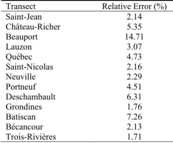
A first-order approximation of the relative errors in observed discharge is provided in Table 1 at 13 measurement transects in the SLFE. Errors in cross-sectional area are neglected in the calculation, assuming that they are one order of magnitude smaller than errors in velocity. The latter are dominated by smoothing and interpolation errors, whose values are provided in
Matte et al. (2014a).
3.2.3 Topographic Data
A DEM is used to compute the wetted area at each time step of the cubature calculation. Topographic data includes channel bathymetry, floodplains, and engineering structures.
Bathymetric data were obtained from the CHS and consist of a mix of high-resolution multibeam echosoundings in the navigational channel and lower-resolution (older) data outside the channel or in shallower areas. To complete the topography in the floodplains, marshes, shoals and intertidal zones, data from LIDAR campaigns conducted during the fall of 2001 and summer of 2012 were used (Matte et al., 2017a; Morin and Champoux, 2006).
Major tributaries were included in the model to allow water to be cyclically stored and evacuated as a function of the tide. Their boundaries were positioned at upstream locations removed from tidal influence. The geometry of the river shores was extracted using geospatial data from Natural Resources Canada’s GeoBase website (http://www.geobase.ca/). Their bathymetry was represented, due to a lack of data, by a regularly shaped trapezoidal channel of constant slope and variable depth and width. Channel depth was determined by calculating the depth needed to discharge the average river flow at an approximate mean velocity of 1 m s-1,
given the local width of the river. Finally, engineering structures, such as bridge pillars, piers, marinas and ports, were also included as topographic elements.
3.3 Model Properties
3.3.1 Harmonic Analyses and Interpolation
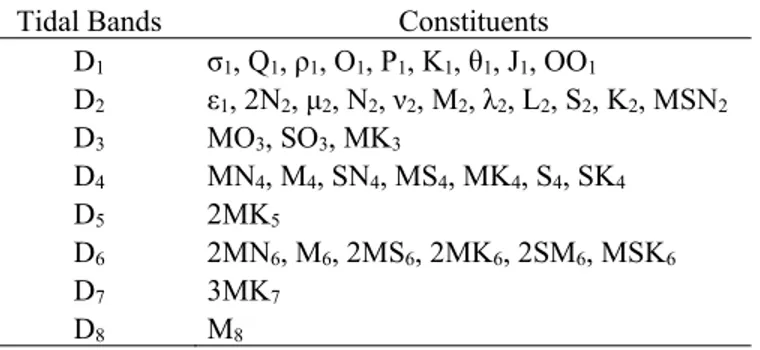
In order to build the 1D spatial model, nonstationary tidal harmonic analyses were performed using NS_TIDE (Matte et al., 2013) on hourly water level data from 13 tide gauges distributed between Saint-Joseph-de-la-Rive and Lanoraie (Table 2), over the 1999–2009 period. The tidal-fluvial model (cf. Eq. (6)) was forced using 39 tidal components, listed in Table 3. The same constituents were included at all stations to allow spatial interpolation of model coefficients throughout the system. Iteratively reweighted least-squares (IRLS) analyses (cf. Eq. (B3)) were performed using a Cauchy weighting function with a default tuning constant of 2.385 (Leffler
and Jay, 2009). Spatial interpolation of model coefficients was carried out between the analysis
stations using piecewise cubic Hermite interpolants (Fritsch and Carlson, 1980), which are continuous up to the first derivatives and preserve monotonicity. The remaining intermediate stations appearing in Figure 1 (shown in italics in Table 2) were used for validation of the
interpolated water levels (cf. Matte et al., 2014b). The overall prediction accuracy of the 1D tidal harmonic model is better than 30 cm in water levels at all stations (Matte et al., 2014b).
The discharge time series Qr (cf. Eq. (4)) used in the analyses are reconstructed by the
method of Bouchard and Morin (2000) (cf. section 3.2.2); they are presented in Matte et al. (2014b). A one-year sample (August 2007 – August 2008) of the time series is provided in Figure 2 (top panel). Differences in discharge between Trois-Rivières and Québec reached a maximum of 8700 m3s-1 in April 2008 during the freshet, due to the contribution of lateral
inflows from tributaries. Minimum and maximum discharges at Québec for the 1999–2009 period were observed in September 2007 (7600 m3s-1) and April 2008 (26 400 m3s-1),
respectively. Historical extreme flows occurred in March 1965 (7000 m3s-1) and April 1976
(32 700 m3s-1) for the 1960–2010 period. Therefore, the chosen 11-year analysis period
represents most of the variability in the modern system.
The station of Sept-Îles, removed from fluvial influence, was used as the reference station for ocean tidal forcing (Figure 1) (cf. Matte et al., 2014b). Daily greater diurnal tidal ranges R were extracted from hourly data at the station. Water levels were high-pass filtered, then re-interpolated using cubic spline functions to a 6-min interval in order to capture the tidal extrema. Tidal ranges R were calculated as the difference between higher high water and lower low water using a 27-h moving window with 1-h steps, then smoothed to eliminate discontinuities,
similarly to Kukulka and Jay (2003a)’s tidal range filter. A sample of the time series is provided in Figure 2 (bottom panel) for the year 2007-2008. Ocean tidal ranges vary approximately between 1.2 and 3.6 m, and get amplified on their way upstream, before being progressively damped as they enter the fluvial estuary.
Further details on the model setup, performance and validation are provided in Matte et
al. (2014b).
3.3.2 2D Mesh and Topography
The 2D finite element mesh used for integration covers a section of the St. Lawrence River extending from Québec (rkm 106.5) to Lanoraie (rkm 302), as shown in Figure 3. It is composed of 178 938 nodes and 342 268 T3 elements and has a 67-m average spatial resolution. The DEM associated with this mesh is presented in Figure 4. The reach between Trois-Rivières (rkm 231) and Québec was taken from a high-resolution hydrodynamic model developed by
Matte et al.(2017a), whereas the Lake Saint-Pierre region was taken from the Montreal –
Trois-Rivières model developed at Environment and Climate Change Canada (Morin and Champoux, 2006). The two grids were respectively truncated at Québec and Lanoraie, and then merged at Trois-Rivières. Discharge variations at the upstream limit are considered as tidally-invariant, although spring-neap oscillations of the MWL are still perceptible at Lanoraie. Amplitude of the semidiurnal tide at this location represents, on average, less than 1% of its amplitude at the SLFE entrance and completely extinguishes during neap tides (Matte et al., 2014b).
For validation with transect data, the mesh was progressively truncated along the surveyed cross-sections (shown in Figure 3), in order to perform each of the discharge reconstructions from the section treated up to the head of the tide.
3.3.3 Cubature Analyses
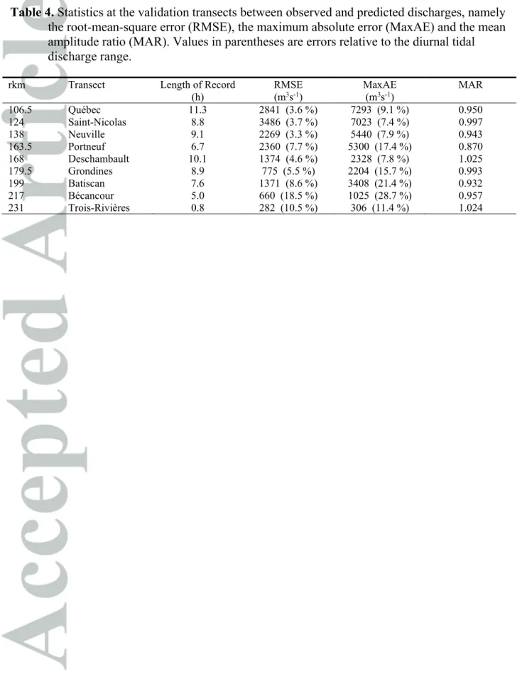
The cubature computations were tested and validated over two periods in June and August 2009, during which the transect data were collected (cf. section 3.2.2). A 6-min time step was used for the input data and discharge computations in order to capture the tidal extrema. Validation of the reconstructed discharges was performed along 9 cross-sections, shown in Figure 3. Statistical goodness of fit criteria were used to assess model performance, including the root-mean-square error (RMSE), the maximum absolute error (MaxAE) and the mean amplitude ratio (MAR) of predicted to observed discharges (Qpred and Qobs, respectively), defined as
follows:
n j obs j j pred Q Q n 1 , , 1 MAR . (10)The MAR is computed using only values of the absolute instantaneous flow exceeding 20 % of the maximum flow, in order to avoid division by near-zero values, similarly to Lefaivre et al. (2016). The error associated with the MAR is defined as (1 – MAR) × 100 %.
In order to illustrate how well the model captures the discharge variability in the SLFE, one-year reconstructions were performed at two contrasting cross-sections: Quebec (rkm 106.5) located in the tide-dominated region and Grondines (rkm 179.5) where tides and MWL are significantly modified by the river discharge. The reconstruction period covers an entire year, extending from August 2007 to August 2008, thus encompassing the tidal range annual
variability as well as a wide range of river discharges (cf. Figure 2), from very low flows (7600 m3s-1) to very high flows (26 400 m3s-1). Two high discharge events occurred in January and
April 2008, approximately lasting two weeks and two months, respectively. These flows are fairly extreme when compared to the average discharge of 12 200 m3s-1 at Québec. The one-year
reconstructions were conducted at a 20-min time step. 4 Results and Discussion
4.1 Validation of the Tidal Discharges
Statistics on the discharge reconstructions made at the validation transects are presented in Table 4. RMSE and MaxAE values cumulate and generally increase from upstream (Trois-Rivières; rkm 231) to downstream (Québec; rkm 106.5), following the increase in extent of the integration domain. However, relative errors (shown in parentheses) tend to decrease as the
variability of tidal discharges gets larger, reaching rRMSE values below 4 % of the diurnal tidal discharge range at downstream locations. Relative errors at upstream locations are less
representative of the actual error since tidal discharge amplitude becomes considerably weaker landward (cf. electronic appendix). Nevertheless, rRMSE are lower than 9 % considering all transects but Bécancour and Trois-Rivières, where the length of the discharge records is less than half the tidal period (Table 4). Another measure of the error made is given by the ratio of
predicted to observed flows, which represents how well the signal amplitudes are reproduced. Values of the MAR are presented in Table 4 for each transect. Estimated tidal discharge amplitudes fall within 7 % of the observed values at all transects but Portneuf (1 – 0.870 = 13.0 %), due to the effects of local channel curvature (see section 4.2.3). Errors associated with the MAR are overall comparable to measurement errors (cf. Table 1); they amount to 4.5 % when averaged over all transects.
Results at the Québec cross-section (rkm 106.5) are presented in Figure 5. On the upper panel are shown the predicted water levels from the 1D tidal harmonic model, which are in good agreement with observations at Québec on June 15, 2009. Variations in the wetted surface area (green dash-dotted curve) illustrate the temporal changes in the entire integration domain, from Québec to Lanoraie. Bottom panel of Figure 5 shows the discharges reconstructed by cubature, compared to transect data acquired over one tidal cycle. Predicted discharges are in good agreement with observations, both in terms of synchronism and amplitude. Slack waters (null discharges) occur slightly after LW and HW at the ebb-to-flood and flood-to-ebb transitions, respectively, indicator of a tidal wave of a mixed character that shares the characteristics of a progressive and a standing wave, typical of alluvial estuaries (Savenije, 2012). The duration of the ebb is almost twice that of the flood at Québec, with discharge volumes approximately two times bigger. Considerable freshwater volumes thus exit the estuary periodically.
Validation at the Deschambault cross-section (rkm 168) is shown in Figure 6. Overall, both predicted water levels and discharges at Deschambault are in good agreement with observations. This region encompasses the largest intertidal areas of the SLFE and is
characterized by a narrow channel of strong currents at the Richelieu rapids. A sharp decrease in wetted surface area starting a few hours before LW occurs at this section. The shape of both the wetted area and water level differs from the curves at Québec, as the tide gets more and more distorted propagating upstream, due to frictional nonlinearities. Current reversals are still observable at Deschambault, although of shorter duration than at Québec. Flood discharges are also more sensitive to the tidal range, being proportionally more weakened than ebb discharges at lower tidal ranges. This results in a larger daily variability of the ratio of flood to ebb volumes as a consequence of the diurnal inequality of the tide.
Validation results for all cross-sections appearing in Figure 3 are provided in an
electronic appendix (Figures S1–S9; from downstream to upstream); they are briefly presented below. At Saint-Nicolas and Neuville (Figures S2–S3), a similarly good fit as Quebec (Figure 5) is obtained. However, some quarter-diurnal oscillations appear in the predicted ebb discharges, not captured in the observations. These may be due to artifacts from the interpolation functions of the 1D tidal harmonic model, which might appear with constituents of higher frequency (shorter wavelength) when the distance separating the stations becomes close to half the constituent wavelength (cf. Discussion in Matte et al., 2014b). At Portneuf (Figure S4), peak flood discharges are underestimated by 5300 m3s-1, which represents 17.4 % of the diurnal tidal
water levels (neither accounted for in the 1D model, nor in the 2D projection), or to the negative bias in predicted water levels during the measured period, especially at HW. Moving past the Richelieu rapids to Grondines (Figure S6), the observed water levels are slightly more distorted than the predicted levels (with earlier HW and later LW). This yields slightly time-shifted flood discharges, but the tidal discharge range remains accurately predicted. In Figure S7, a negative bias in predicted water levels of ~20 cm is observed at Batiscan, which is within the prediction accuracy of the nonstationary tidal harmonic model (<30 cm) (Matte et al., 2014b). This results in slightly underestimated and time-shifted flood discharges, whereas ebb discharges are well reproduced. At Bécancour (Figure S8), a positive bias in the predicted tidal signal is obtained along with a less pronounced asymmetry. As a result, the predicted tidal discharges present a larger variability than observed, with lower and time-shifted flood discharges. The measured discharge time series at Trois-Rivières (Figure S9) is very short, which makes it hard to assess the quality of the estimates at this location. With a negative bias in water levels of less than 10 cm (for a tidal range varying between 10-20 cm during the observed period), the discharges are slightly overestimated, but the impact on tidal discharge range cannot be evaluated.
4.2 One-Year Tidal Discharge Reconstructions 4.2.1 Wetted Surface Areas
Plots of the cumulative wetted surface area for each transect are presented in Figure 7 for the 2007-2008 period. The inundated area (or, equivalently, the integration domain) varies both longitudinally and in time as a function of river discharge and local tidal range (cf. Figure 2). At low discharges, the wetted surface area considerably reduces, mainly due to the presence of a fluvial lake upstream, characterized by an extensive floodplain. This surface is progressively augmented moving downstream and generally increases with MWL during high discharge events, due to the flooding of intertidal flats. The wetted surface area also exhibit semidiurnal variations that follow the amplitude of the tide. The latter varies with river flow, so that semidiurnal fluctuations in wetted surface area are generally stronger during periods of low discharge. Furthermore, fortnightly and monthly variations in tidal range translate into variations in wetted areas with the same periodicity. However, these fluctuations tend to diminish past a certain discharge value. Reasons for this reduction may include the attenuation of the low-frequency tides with discharge, but most likely arise mainly from the presence of steeper topography in the intertidal zone above a certain level (e.g., due to bank enrockment).
Differences between the maximum and minimum wetted surface areas at a given location give some indication of – but do not exactly correspond to – the total extent of intertidal flats upstream. In fact, because of the time lags associated with the landward propagation of the tide, shallow areas are not flooded or dried synchronously throughout the system.
4.2.2 Tidal Discharges
Time series of reconstructed tidal discharges are presented in Figures 8 and 9 at Québec (rkm 106.5) and Grondines (rkm 179.5) for the 2007-2008 period. Tidal discharges at Québec (Figure 8) show a large semidiurnal variability. Ebb (positive) discharges are about five times the daily average (in red) during spring tides, exceeding 50 000 m3s-1 under average flow conditions.
During neap tides, ebb tidal discharges are slightly below 40 000 m3s-1. Flood (negative)
discharges are overall stronger than ebb discharges during spring tide, reaching almost -60 000 m3s-1 under average flow conditions. During neap tides, however, they are significantly more
reduced than ebb discharges, with values nearly as low as -20 000 m3s-1. Ebb discharges overall
last longer than flood discharges, with ebb volumes approximately twice as large as the flood volumes on average, thus yielding a net seaward outflow.
Seasonal variations also appear in the reconstructed signal at Québec as a function of the river flow. During high flow conditions, the strength and duration of ebb (flood) discharges are increased (reduced). Ebb tidal flows can exceed 60 000 m3s-1, representing more than twice the
daily net outflow. When conditions of very high flow and neap tides are combined, near zero and very short flood discharges may occur, as observed at the end of April 2008, meaning that there is no current reversals occurring beyond Québec. While the upstream limit of current reversals is generally located between Grondines (rkm 179.5) and Bécancour (rkm 217) (Matte et al.,
2017b), under extreme conditions this limit can be displaced much further seaward (some 60 rkm downstream of Grondines in this case).
Tidal discharges at Grondines (rkm 179.5) are presented in Figure 9. This station is located past the Richelieu rapids in the transition zone between the tidal and tidal-fluvial reaches of the SLFE (Matte et al., 2014b). The influence of the upstream river discharge on tidal
discharge variability is drastically increased, compared to the signal at Québec; tidal amplitudes are reduced and tidal asymmetry is enhanced. This results in dynamical changes in the ebb-flood characteristics. Globally, ebb tides last longer than flood tides and the increase in water levels is much shorter and abrupt during flood tides than at downstream locations. Departure of flood discharges from the net average flow is therefore much more important than ebb discharges, but occurs on a shorter time period. During very low discharges (September 2007), current reversals take place during both spring and neap tides, although only during the lowest low water (LLW) in the latter case, because of the diurnal inequality in tidal ranges. During high discharges (January and April 2008), the amplitude of the variations in tidal discharge is significantly reduced, following the decrease in tidal range. While the range of variability approximates 25 000 m3s-1 in periods of low discharge, they barely exceed 5 000 m3s-1 at high discharge.
Furthermore, when the mean flow reaches about 15 000 m3s-1, no more current reversals are
observed, even during spring tides, although velocities still experience a significant reduction with the rising tide.
These results highlight the capacity of the model to capture tidal discharge variability under contrasting tidal-fluvial conditions along the river, for a wide range of temporal scales, including intratidal, fortnightly and seasonal. Important tidal flow characteristics are represented by these estimates, such as the times of slack water, maximum ebb and flood discharges, the diurnal inequality in tidal discharges, neap-spring storage effects, and the displacement of the upstream limit of current reversals as a function of river flow and tidal range.
4.2.3 Error Analysis
To evaluate the significance of the tidal discharge reconstructions, error sources were identified and an error analysis was performed based on Eq. (9). From the validation of Morse’s estimates of drainage areas (cf. section 3.2.2, Boudreau and Fortin, 2018), an error of 100 m3s-1
was attributed to upstream and lateral inflows (Qr) for tributaries between Lasalle and
Trois-Rivières. Because no comparison was made between Morse’s calculations and the updated (2017) formulas downstream of Trois-Rivières, this estimate was simply doubled to 200 m3s-1 to
include potential biases downstream as well as random errors from the stage-discharge relations used. Imperfect conceptual representation of the watersheds hydrology may also contribute to the
overall inaccuracy, but the lack of validation data in the St. Lawrence River prevents us from further quantifying the error in the reconstituted discharge time series for tributaries.
Despite the advantages of using a 1D tidal harmonic model to represent water levels rather than direct observations (see next section), such a strategy comes at the price of added errors in the tidal discharge estimates that arise from model uncertainties. These are partly associated with the model underlying assumptions and approximations (cf. Appendix B), and partly due to interpolation errors of the tidal constituent properties. Resulting uncertainties in predicted water levels translate into volume errors and temporal offsets of the predicted
occurrence of current reversals. The synchronicity of the tidal discharges may also be affected by errors in tidal asymmetry.
Random errors associated with tidal measurements contribute to the uncertainty in tidal estimates at the analysis stations and were quantified using the correlated noise model
implemented in NS_TIDE (Matte et al., 2013). For the analysed period (1999-2009), these errors translated into RMSE in water levels varying between 0.15 and 0.29 m at the analysis stations. Errors due to spatial interpolation of the tidal coefficients were estimated to vary between 0.11 and 0.30 m, which is comparable to the analysis error. These errors result in RMSE in tidal range varying between 0.02 and 0.44 m (maximum at Saint-Nicolas (rim 124)) and in RMSE in MWL ranging between 0.11 and 0.25 m (maximum at Cap-Santé (rkm 157)), depending on the station (Matte et al., 2014b). In comparison, the dynamic range in water levels varies approximately from 3.5 m upstream (Trois-Rivières) to 6 m downstream (Québec), considering the combined effects of tides and river flow. For use in Eq. (9), mean values of 0.15 and 3 m were used for δR and R, respectively, representing an estimate of the average longitudinal variability in these parameters. MWL biases, on the other hand, only affect the wetted superficies and were estimated to be approximately 0.16 m on average.
Additional errors also include unresolved phenomena by the tidal harmonic model, which may not fully resolve the nonstationary tidal content. More particularly, the harmonic model has never been tested under very nonstationary conditions (e.g., rapid flood); its performance in such a context thus remains to be assessed. Furthermore, the model does not account for the effects of winds and storm surges. Winds are especially important in Lake Saint-Pierre and may
significantly affect the storage volumes. Also, in many estuaries, storm surges can have a “tide-like” signal and they thus add energy in the tidal frequency band as well as at the low frequency end of the spectrum. In its current form, the accuracy of the model is therefore best during non-storm conditions and during periods of weak to moderate non-stationarity. Inclusion of these phenomena should be carried out in the future, either by directly incorporating these variables in the model basis functions (Eq. (6)) or by using more sophisticated functions to spatially
interpolate the tidal constituents and residual (unresolved tidal or non-tidal) water levels (e.g.,
Hess, 2003; Shi et al., 2013).
Lateral variations in water levels in the vicinity of river bends can also yield increased errors in tidal discharge estimates (e.g., Portneuf; Table 4), as they are not accounted for by the 1D model. These lateral water level gradients can be considerable in meandering rivers of high sinuosity (Hidayat et al., 2011) as well as between the channel and floodplains (Jay et al., 2016;
Jay et al., 2015; Matte et al., 2017b). (Matte et al., 2017b) investigated lateral variability in the
SLFE using a 2D hydrodynamic model, corroborated by field measurements at a series of transects (Matte et al., 2014a). They showed that, in some cross-sections where tidal flats represent a significant percentage of the total river width (e.g. Deschambault, Grondines), the
water levels were nearly the same between the channel and floodplain at HW, whereas the largest lateral gradients were observed near LW (approximately ~0.1 m). Interestingly, while near-LW lateral gradients are the largest, this does not coincide with the largest dh/dt (which typically occurs on early ebb or early flood). Overall, the most significant lateral gradients were observable during the falling tide (ebb), as the tidal flats were emptying into the channel,
whereas virtually no lateral gradients were observed during the rising tide (flood). As a result of this asymmetric behavior, most of the error is biased towards LW and does not average out over a tidal cycle.
In this method, the use of a 2D geometry is crucial in adequately representing the wetting-drying of the integration surface for the computation of accurate tidal volumes. Topographic errors associated with imprecision in the raw data, vertical datum, dynamic morphology and the chosen spatial discretization (i.e. finite elements) therefore represent additional sources of uncertainty. Moreover, natural and anthropogenic changes in river
morphology should be accounted for if long-term historical reconstructions are envisaged, since historic floodplain bathymetry is often very different from modern bathymetry. In the present application, LIDAR data have an expected accuracy of 0.15 m, but the other sources of topographic inaccuracies are hard to quantify. A combined vertical error of 0.2 m therefore seemed to be a reasonable estimate for the floodplains, averaged over the entire domain.
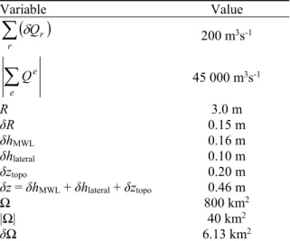
In sum, systematic errors in water levels and topography, although they virtually have no effect on the time derivative of h (cf. Eq.(5)), may significantly affect the computed wetted superficies. By combining the estimated biases in MWL (0.16 m), lateral slopes (0.1 m) and topography (0.2 m), we arrive at an estimate of the vertical error δz of 0.46 m. By inspection of Figure 7, it is possible to estimate the average error in wetted surface area from the calculated vertical bias, as follows. Under average discharge conditions, i.e. Qr ~ 12 000 m3s-1 at Québec
(e.g., in February 2008; Figure 2), the cumulative wetted surface area Ω at Québec amounts to approximately 800 km2, with a range of variability |Ω| over the semi-diurnal tidal cycle of about
40 km2 (Figure 7). Assuming that the error ratios of wetted surface area to vertical bias, i.e.
δΩ/δz, are comparable to the range ratios of wetted surface area to tidal range, i.e. |Ω|/R, the
uncertainty in wetted surface area can be approximated as: z R
~ . This yields an error estimate for δΩ of 6.13 × 10⁶ m2.
Under mean discharge and tidal range conditions, the amplitude over a tidal cycle of the summed elemental discharges,
e e
Q , is approximately 45 000 m3s-1 (Figure 8). Solving Eq. (9)
using the uncertainty estimates provided above (summarized in Table 5), the tidally-averaged error in computed discharges is estimated to equal 2285 m3s-1. This corresponds to a relative
error of 2.5% of the average tidal discharge range at Québec (~90 000 m3s-1), which is
comparable to validation results obtained at the Québec cross-section between predicted and ADCP-derived discharges (cf. Table 4).
In the present calculation, the error is dominated by uncertainties in tidal ranges by one order of magnitude compared to errors in the river discharges and wetted surface areas.
Uncertainty in tidal ranges is mostly driven by the tidal harmonic model. Under high flow conditions, however, the contribution of the river discharge uncertainty may become of equal
importance to the tidal range error, as suggested by the revised estimates of drainage areas (cf. section 3.2.2, Boudreau and Fortin, 2018).
4.3 Benefits and Limitations of the Method
Although it does not capture lateral gradients, benefits of using a 1D tidal harmonic model to represent water levels include the ability to fill temporal gaps in the data (e.g., top panel of Figure 6), to spatially interpolate tidal coefficients between stations, to carry information about the physics and to make tidal discharge forecasts. The descriptive and predictive capabilities of the tidal harmonic model are therefore passed on to the reconstructed tidal
discharges, so that they can be estimated under virtually any river discharge (Qr) and ocean tidal
range (R) conditions. Furthermore, the availability of long tidal records at various locations within estuaries provides the opportunity to reconstruct long and continuous past flow records from historic water level data, provided that sufficient information on the historic evolution of floodplain bathymetry is available. Compared to direct measurements, these cubature
computations can be performed at any river sections, as opposed to the installation of fixed apparatus (e.g., H-ADCP), usually limited in number. They can also be used to evaluate flows during flood conditions, when discharges exceed by far the calibration range of both H-ADCPs and traditional rating curves, or in cases of instrument failure. Moreover, this method could potentially be used to improve flow estimates in deltas, such as the NDOI estimate made in San Francisco Bay.
With a 2D discretization of the domain, serving as a descriptor of the river geometry, these components both represent added complexity to a generally simple method. It requires accurate estimations of the upstream freshwater discharge, a sufficient number of tide gauges to allow spatial interpolation of the tidal properties and detailed topographic data over shallow intertidal areas. In large rivers, however, the availability of such data is becoming more and more common, especially along navigation pathways. While the elaboration of a 2D finite element mesh may be a laborious task, this newimplementation of the method of cubature represents a significant simplification over traditional numerical models, as it only involves regression analyses for the determination of harmonic coefficients and resolution of the continuity equation over a discretized domain, with no parameterization of the friction properties. Computing time and sensitivity to bathymetric errors are thus expected to be substantially lower than with full 2D numerical models. On the other hand, lateral slopes may arise from phase lags and amplitude differences of the tidal flows between the channel and floodplains. These are not accounted for by this method, which may become a significant drawback in presence of extensive shallow areas.
5 Conclusion
Previous attempts to compute tidal discharges in the SLFE either offered limited accuracy or a too high computational cost for real-time and historical analyses. For instance, the cubature estimations made by Forrester (1972) did not account for time variations in the surface and cross-sectional areas with tides and river flow, which significantly affect the total mass balance in presence of tidal flats. Similarly, a large number of numerical models have been developed (see, e.g., Matte et al. (2017a) for a review of existing models), but most of them only
reproduced qualitatively the main tidal and fluvial characteristics of the SLFE, due to a lack of validation data and imprecise discharge boundary conditions. In comparison, high-resolution
models of higher dimensions (2D, 3D), despite their improved accuracy, are generally not suited for long-term analyses (e.g., Matte et al., 2017a; b).
An adaptation of the method of cubature for the computation of tidal discharges was presented and applied to the SLFE, integrating the continuity equation for discharges at different sections. Tidal heights were spatially interpolated between stations by reconstruction of tidal coefficients from a 1D nonstationary tidal harmonic model, thus filling temporal gaps in the tidal data and allowing information on tidal properties to be passed on to the flow estimations. The 1D longitudinal model was expanded laterally and projected on a 2D finite element mesh in order to compute the time-varying wetted surface area, based on detailed topographic data over intertidal flats. Discharge time series were reconstructed at 9 cross-sections in the SLFE and validated against recent discharge data, reaching rRMSE values below 4 % of the diurnal tidal discharge range at downstream locations and below 9 % upstream, with the exception of two transects with shorter records. On the other hand, the error made based on the ratios of predicted to observed flows amounted to 4.5 % when averaged over all transects. Overall, both the synchronism and variability of the observed data were well reproduced by the model. One-year reconstructions conducted at two cross-sections of the SLFE also showed the potential of the method for dynamical inquiries along the tidal-river continuum. The model was able to reproduce the tidal discharge variability at a wide range of temporal scales and under contrasting tidal-fluvial conditions.
This method provides a new means for efficiently and accurately estimating tidal discharges in estuaries. It can be used to issue short-term forecasts (given that upstream river flow can be predicted with sufficient accuracy), in conjunction with discharge measurement stations or as an alternative to the development of dynamic rating curve models. Furthermore, dynamical insights can be gained from historical reconstructions of tidal discharges, with numerous implications from a water resources management perspective, both in terms of water quality and quantity.
Appendix A: Derivation of Observed Discharges from Water Level and Velocity Data Transect data consisting of water level and velocity measurements were obtained in the SLFE by Matte et al. (2014a), who devised a procedure to reconstruct continuous and synoptic fields from non-synoptic RTK GPS and ADCP data. These fields are used to compute the
observed time-varying discharges and section-averaged tidal currents. The calculation consists of the following steps:
1. The bed elevation zb (in m) along each transect is obtained by subtracting the
instantaneous ADCP water depths, HADCP, from the water levels measured by the RTK
GPS, hRTK:
ADCP RTK
b h H
z ; (A1)
2. The gridded bathymetry points from each crossing are interpolated in time (yielding zint)
to account for deviations of the boat from the mean transect line (Figure A1), similarly to the interpolation of velocities (see Matte et al.(2014a) for details on the procedure; an example of the interpolated bathymetry field is presented in Figure A2):
int grd
b z z
z gridding interpolation