Upper Bounds for Large Scale Integer Quadratic Mulitdimensional Knapsack Problems

UPPER BOUNDS FOR LARGE SCALE INTEGER QUADRATIC

MULTIDIMENSIONAL KNAPSACK PROBLEMS

Dominique Quadri1, Eric Soutif2, and Pierre Tolla1 1

LAMSADE Université Paris-IX

Place du Maréchal de Lattre de Tassigny 75775 Paris Cedex 16, France

2

CEDRIC

Conservatoire National des Arts et Métiers 292 rue Saint-Martin

75003 Paris, France

Corresponding author. E-mail: Eric.Soutif@cnam.fr

Abstract: We consider the separable quadratic multi-knapsack problem (QMKP) which consists in maximizing a concave separable quadratic integer function subject to m linear capacity constraints. The aim of this paper is to develop an effective method to compute an upper bound for (QMKP) from a surrogate relaxation originally proposed in Djerdjour et al. (1988). We evaluate the quality of three other upper bounds for (QMKP) and compare them theoretically and experimentally with the bound we suggest. We also present an effective heuristic method to obtain a good feasible solution for (QMKP). Finally, we report computational experiments that assess the efficiency of our upper bound for instances up to 2000 variables and constraints.

Keywords: Integer programming; Separable quadratic programming; Multidimensional Knapsack Problem; Surrogate relaxation.

1. INTRODUCTION

This paper presents a method to compute a good upper bound for the separable quadratic multi-knapsack problem (QMKP), which is derived from the solution method developed by Djerdjour et al. (1988). The problem we examine is a generalization of the integer quadratic knapsack problem (QKP) which consists in maximizing a concave separable quadratic integer function subject to a single linear capacity constraint. Although there is a paucity of solution methods to (QKP), significant contributions may be found in the literature. Among these, Mathur et al. (1988) solve (QKP) to optimality by applying a piecewise linearization to the objective function to obtain an equivalent 0-1 linear problem. Bretthauer and Shetty suggest several effective methods, such like pegging algorithms (2002a) and projection methods (1996 and 2002b) to solve the LP-relaxation of (QKP) so as to compute an upper bound of the optimal value in a fast CPU time.

The main application of (QKP) is in finance (Mathur et al., 1988, Bretthauer and Shetty, 1997) for the portfolio management problem can be formulated as a mathematical program with a quadratic objective function under a knapsack constraint (Markowitz, 1952). The quadratic function measures both the expected return and the risk and the single knapsack constraint represents the budget constraint. The assumption of a single knapsack constraint does not allow the possibility of investing into assets of different risk levels. This can be formulated by means of several knapsack constraints, each representing a budget allocated to assets of a given risk level. We therefore face an integer quadratic multi-knapsack problem (QMKP) which is a generalization of (QKP). This

capital budgeting model is discussed in Djerdjour et al. (1988) and Faaland (1974). Formally the integer (non pure binary) quadratic multidimensional knapsack problem (QMKP) can be written as:

( )

⎪ ⎪ ⎪ ⎩ ⎪ ⎪ ⎪ ⎨ ⎧ = = ≤ ≤ = ≤ = − =

∑

∑

∑

= = = n j x n j u x m i b x a x f x d x c x f QMKP j j j n j ij j i n j n j j j j j j j , , 1 integer, , , 1 , 0 , , 1 , t. s. ) ( max ) ( ₁ 1 1 2 K K K

where the coefficients c_j, d_j, a_ij, b_i are nonnegative. The bounds u_j of variables x_j are pure integers, with

(

j j

)

j c d

u ≤ /2 . Indeed, the separable objective function is concave which implies that for all fj, x*j ≤

(

cj/2dj

)

, where x*j is the optimal solution of the program max0≤xj≤uj fj

( )

xj .

The integer quadratic multidimensional knapsack problem (QMKP) has received less attention in the literature than (QKP). To the best of our knowledge, Djerdjour et al. (1988) are the only authors to propose a specific solution method to solve (QMKP). As such, their method is more effective than more general techniques that have been primarily developed to solve general integer quadratic programs (see Cooper, 1981 and Körner 1985, 1990).

The method of Djerdjour et al. first consists in a piecewise linearization of the objective function which consequently converts (QMKP) into an equivalent 0-1 multidimensional knapsack problem, (MKP), for which a wide range of methods exists (see for instance Fréville and Plateau, 1986 and Chu and Beasley, 1998). These methods are presented and analyzed in the recent survey of Fréville and Hanafi (2005). Djerdjour et al. then apply a surrogate relaxation to the m constraints of (MKP) in order to compute an upper bound of the objective function of (QMKP).

In this paper we propose an upper bound that improves the surrogate relaxation originally proposed by Djerdjour et al. (1988). The bound is improved from both a qualitative and a computational standpoint. We also develop a heuristic method to get a feasible solution to (QMKP). As no numerical evaluation of the quality of the bounds for (QMKP) is available in the literature, we provide a theoretical and experimental comparison of the different bounds described in this paper. We will compare the LP relaxation, a linearization, the surrogate relaxation (Djerdjour et al., 1988) as well as the upper and lower bounds we propose. The objective of the computational study we conduct in this paper is to determine which bound is finally the most appropriate to be used in a branch-and-bound procedure to efficiently solve the problem. To this purpose we consider instances up to 2000 variables and 2000 constraints. Simulation results show that our method provides an upper bound of good quality in most cases and is always better than the surrogate relaxation (Djerdjour et al., 1988) while requiring a significantly less computational time.

The paper is organized as follows. Section 2 summarizes the algorithm proposed in Djerdjour et al. (1988) to compute an upper bound of (QMKP). In Section 3, we present two improvements of this algorithm. The first improvement is meant to speed up the computation of the bound and the second one increases the quality of the bound. A feasible solution is proposed in Section 4. The computational results are reported in Section 5. In section 6 we summarize the main results of this paper and we point out some directions for further research.

In the remainder of this paper, we adopt the following notations: letting (P) be an integer or a 0-1 program, we will denote by ( P ) the continuous relaxation problem of (P). We let Z[P] be the optimal value of the problem (P) and Z[ P ] the optimal value of ( P ).

2. THE ALGORITHM OF DJERDJOUR, MATHUR AND SALKIN (1988)

The method proposed by Djerdjour et al. (1988) is an exact method to solve (QMKP). At each node of the search tree, an upper bound is computed by solving a polynomial problem derived from (QMKP). First, an equivalent formulation of (QMKP) is obtained by using a direct expansion of the integer variables x_j as originally proposed by Glover (1975) and by applying a piecewise linear interpolation to the initial objective function as discussed by Mathur et al. (1983). Consequently, (QMKP) is equivalent to the 0-1 piecewise linear program (MKP):

(

)

(

)

{ }

⎪ ⎪ ⎩ ⎪⎪ ⎨ ⎧ = = ∈ = ≤ =

∑

∑

∑ ∑

= = = = 1 1 , 1 , 0 , , 1 , t. s. ) ( max ) ( 1 1 1 1 j jk n j i u k jk ij n j u k jk jk ,u , ,n, k , j y m i b y a y s y l MKP j j K K K where

( )

j u kj n jk y y ,..., 1 ,..., 1 = = =

,

∑

u₌j = k 1yjk xj, sjk = fjk− fj,k−1 and 2 k d k c f_jk = _j − _j .

In the second step of the algorithm, a surrogate relaxation is applied to the LP-relaxation of (MKP). The surrogate relaxation initially introduced by Glover (1965) consists in aggregating the m initial linear constraints into a single constraint, namely a surrogate constraint, by replacing the set of constraints Ay≤b with a unique constraintwAy≤wb, where A stands for the matrix of constraints of (MKP). The vector w=(w₁,_K,w_i,_K,w_m)

is nonnegative and is called the surrogate multiplier. The resultant formulation (KP, w) is the surrogate relaxation problem of (MKP) and is written as:

The above problem (KP,w) is a knapsack problem whose LP relaxation may efficiently be solved in

O(n’log2(n’)) operations, where n’ stands for the number of variables of (KP, w). The knapsack problem (KP,w)

is one of the most common problems examined in the operations research literature (see Martello and Toth, 1990). As proved by Glover (1965), (KP, w) is a relaxation of (MKP). The proof relies on the fact that an optimal solution of (MKP) is feasible for (KP, w). Assuming that y* is an optimal solution of (MKP), the following inequalities hold:

(

)

i

m j u k jk ij y b a j _≤

∑

=1

∑

=1 *

for all i=1,…,m. Multiplying each previous inequality with

wi≥ and then summing all these inequalities lead to show that y0 * satisfies constraint (1). Consequently y* is feasible (but not necessary optimal) for (KP, w). In addition both objective functions of (MKP) and (KP, w) are identical, which completes the proof.

(

)

[

]

{ }

⎪ ⎪ ⎩ ⎪⎪ ⎨ ⎧ = = ∈ ≤

∑

∑

∑

∑

∑ ∑

= = = = = = 1 1 , 1 , 0 ) 1 ( t. s. max ) , ( 1 1 1 1 1 1 j jk n j m i i i u k jk m i i ij n j u k jk jk ,u , ,n, k , j y b w y a w y s w KP j j K K

For any value of w≥0 the optimal value Z

[ ]

KP,w of

(

KP,w

)

is an upper bound of the optimal value

[ ]

MKP

Z of

( )

MKP . Solving the dual surrogate problem: minw≥0 Z

[ ]

KP,w denoted by (SD), leads to find the

best upper bound Z

[

KP, w*

]

. Since the objective function of (SD) is quasi-convex the authors use a local descent method that provides a global minimum w*.

3. IMPROVING THE UPPER BOUND

We present two improvements of the method in Section 2 to compute an upper bound for (QMKP). We chose to keep the surrogate relaxation of (MKP) initially used by the authors although a Lagrangean relaxation could have been implemented. The rationale for using a surrogate relaxation rather than a Lagrangean relaxation stems from theoretical results which show the superiority of the former over the latter (Fréville and Hanafi, 2005).

First, the local search descent method originally used by Djerdjour et al. to compute the optimal surrogate multiplier is abandoned for a global method which is proved to be faster as evidenced by the computational results presented in Section 5. The second improvement proceeds from an additional stage in which we solve (KP,w*) in 0-1 variables rather than in continuous variables. We finally establish an order relation between all the upper bounds included in the experiment for the sake of comparison.

The first improvement is derived from the following proposition.

Proposition 1 If w*≥0 is the dual optimal solution of

( )

MKP then the optimal value of

( )

MKP is equal to the

optimal value of

(

KP, w*

)

, that is:

[ ] [

MKP Z KP, w*

]

Z =

and w* is an optimal surrogate multiplier for (SD)=min_w≥0 Z

[

KP,w

]

.

Proof The proof involves two parts. We first show that Z

[ ] [

MKP ≥ZKP, w*

]

. We then establish that

[ ] [

MKP ZKP, w*

]

Z ≤ .

Let c’ and A’ be the cost vector and the constraints matrix of

( )

MKP , respectively. Let us denote by e and I the unit vector

(

te=

(

1,_K,1

)

)

and the identity matrix, respectively. The problem

( )

MKP and its dual

(

DMKP

)

can be written as:

(

)

₍

(

)

₎

⎪ ⎪ ⎩ ⎪⎪ ⎨ ⎧ ≥ → ≤ → ≤ 0 y . var . var ' t. s. max v dual e y u dual b y A c'y MKP ⎪⎩ ⎪ ⎨ ⎧ ≥ ≥ ≥ + = + 0 , 0 ' ' t. s. min ) ( v u c v I uA ve ub g(u,v) DMKP

⎪⎩ ⎪ ⎨ ⎧ ≤ ≤ ≤ = 0 ' t. s. max ) , ( e y wb y wA c'y h(y) w KP

(

)

⎩ ⎨ ⎧ ≥ 0 min w KP,w Z (SD)

We first prove the following statement:

. 0 ) , ( ) , ( ) ( ) , ( ≥ ≥

∀ uv feasible for DMKP then g uv Z KP u

Let (u,v) be a feasible solution for

(

DMKP

)

and yu the optimal solution for

( )

KP,u . We have

ve y uA ve ub v u

g( , )= + ≥ ' _u+ as ub≥uA'y_usince yu is a feasible solution for

( )

KP,u . In addition,

0 '

'≥c−v and y_u ≥

uA , as (u,v) is feasible for

(

DMKP

)

, which implies that g(u,v)≥ 'c y_u −vy_u +ve. From the previous inequality we obviously have g(u,v) ≥ c'yu with c'yu =Z(KP,u) as 0≤ yu ≤e.

We let (u*,v*) and w* denote the optimal solution for

(

DMKP and for (SD) respectively. From the duality in

)

linear programming, we know that: Z

( ) (

MKP =Z DMKP

)

. Consequently the following inequalities hold:

( ) (

)

( *, *) , * min ₀

(

,

)

, *⎟ (2) ⎠ ⎞ ⎜ ⎝ ⎛ = ≥ ⎟ ⎠ ⎞ ⎜ ⎝ ⎛ ≥ = =Z DMKP g u v Z KPu _≥ Z KPw Z KPw MKP Z w

The second part of the proof consists in showing that

( )

⎟

⎠ ⎞ ⎜ ⎝ ⎛ ≤ * , w KP Z MKP

Z which is straightforwardly obtained since

(

KP, w*

)

is a (surrogate) relaxation of

( )

MKP as proved at the end of Section 2. We therefore have shown

that

( )

⎟ ⎠ ⎞ ⎜ ⎝ ⎛ = * , w KP Z MKP Z .

In addition, the expression (2) includes the following result:

(

)

⎟ ⎠ ⎞ ⎜ ⎝ ⎛ ≥ ⎟ ⎠ ⎞ ⎜ ⎝ ⎛ ≥ = * * * * , , ) , (u v Z KPu Z KP w g DMKP Z

From (2) we know that

(

)

⎟ ⎠ ⎞ ⎜ ⎝ ⎛ = * , w KP Z DMKP

Z . It follows that u* is an optimal multiplier for the surrogate

dual problem (SD). †

Proposition 1 also appears in Martello and Toth (2003) but no proof had been brought. From This proposition an optimal vector w* can be obtained by solving the dual of

( )

MKP instead of using the local descent method suggested by Djerdjour et al. The numerical results presented in Section 5 assess the computational efficiency of this alternative way for computing w*. To improve the upper bound Z

[

KP, w*

]

we propose an additional stage in which we use w* computed as previously described. This stage consists in solving (KP,w*) in 0-1 variables rather than in continuous variables. In other words we compute Z[KP,w*] instead of Z

[

KP, w*

]

. An outline of the algorithm to obtain our improved upper bound is reported in Figure 1.

1. Transform (QMKP) into an equivalent 0-1 piecewise linear formulation (MKP). 2. Solve the dual of the continuous relaxation of (MKP) to obtain its optimal solution w*. 3. Consider the surrogate relaxation of (MKP) using w*, say its surrogate problem (KP,w*). 4. Solve (KP,w*), to get its optimal value Z[KP,w*].

5. Return Z[KP,w*].

Remark 1 If the optimal solution of (KP,w*) is feasible for (QMKP) then Z[KP,w*] is the optimal value of

(QMKP).

It follows from Remark 1 that the value of the bound will actually be the optimal value of several instances in our experiments.

Classically the optimal value Z

[

QMKP

]

of the continuous relaxation of (QMKP) is used as an upper bound for (QMKP). This value Z

[

QMKP

]

can easily be computed by using a commercial software, since Z

[

QMKP

]

is a concave problem (the quadratic and separable objective function is positive semi-definite and the feasible set is convex). The following proposition shows that the upper bound of Djerdjour et al. (1988) and our improved upper bound are always better than Z

[

QMKP

]

.

Proposition 2 The optimal value of the continuous relaxation of (MKP) is never worse than the optimal value of

the continuous relaxation of (QMKP), that is:

[ ] [

MKP ZQMKP

]

Z ≤ .

Proof Let y* be an optimal solution of

( )

MKP and let l( y*) be its objective value. From y* we derive a feasible solution feasible but not necessarily optimal for

(

QMKP

)

and such that l(y*)≤ f(~x), by setting:

{

n

}

j y x j u k jk j , 1, , ~ 1 * K ∈ ∀ =

∑

= .

As y* is feasible for

( )

MKP , it verifies:

∑

n_j=1a_ij

(

∑

u_k=j₁y*_jk

)

≤b_i,∀i∈

{

1,K,m

}

and y_j∈

[ ]

0,1,∀j∈

{

1,_K,n

}

. Therefore, replacing

(

∑

u_k=j₁y*_jk

)

with x~_j we get:

∑

n_j=1a_ij~x_j ≤b_i,∀i∈

{

1,K,m

}

and 0≤x~_j≤u_j, ∀j∈

{

1,K,n

}

. So ~ is feasible for x

(

QMKP

)

.

Let us now show that l(y*)≤ f(~x). Recall that l(y)=

∑ ∑

n_j=1 u_k=j1sjkyjk and that =

∑

= − n j cjxj djxj x f ₁ 2 ) ( . It

suffices to prove that:

{

n

}

j y s x d x c j u k jk jk j j j j~ ~ , 1, , 1 * 2 K ∈ ∀ ≤ −

∑

= (3) Noting that:

[

² ( 1) ( 1)

]

, ) ( 1 * 2 1 * 1 , 1 *

∑

∑

∑

= = − = − + − − − = − = j j j u k j j j j jk u k jk jk jk u k jk jk y k d k c k d k c y f f y s

we get with some easy algebra:

∑

∑

= = − − = j j u k u k jk j j j jk jky c x d k y s 1 1 * * ) 1 2 ( ~ ₍₄₎

Moreover, developing ~x2j we get:

(

∑

)

∑

₌

∑ ∑

₌

− = = = + = j uj j k u k k k jk jk jk u k jk j y y y y x _{1 1} 1 1 ' * ' * 2 * 2 1 * 2 2 ~ _.

Noting that y*_jk2 ≤y*_jk since y*_jk∈

[ ]

0,1 , and that

∑

−_'=1₁ *' ≤ −1

k

k yjk k for the same reason, we get:

∑

∑

∑

= = = − ≤ − + ≤ j j j u k jk j u k u k jk jk j y k x k y y x 1 * 2 1 1 * * 2 ) 1 2 ( ~ ) 1 ( 2 ~ (5) Inequalities (4) and (5) imply inequality (3). Thus y* and x~ verify:

[ ]

MKP l(y*) f

( )

~x z

[

QMKP

]

.

Figure 2 illustrates the relationship between the four upper bounds.

Figure 2. Comparison of the upper bounds

4. AN EFFICIENT HEURISTIC TO COMPUTE A FEASIBLE SOLUTION

In this section we propose an algorithm to compute a lower bound for (QMKP). This bound will be used to assess the quality of our improved upper bound as well as the existing upper bounds.

The main idea of the proposed heuristic is the following. We first consider the optimal solution y* of

( )

MKP . Letting _j =

⎣

∑

u_k=j y_jk

⎦

1 *

α , for each variable x_j of (QMKP), where

⎣ ⎦

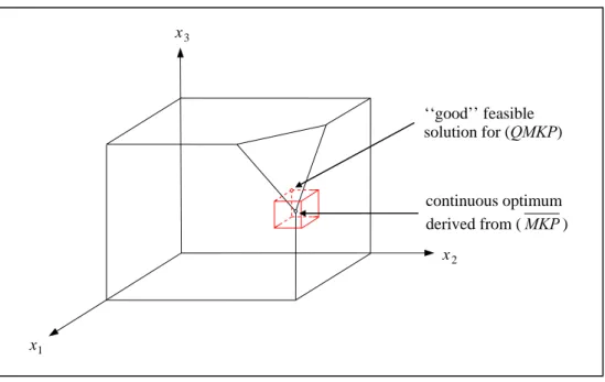
x denotes the biggest integer smaller than or equal to x, we add to (QMKP) the constraint αj ≤xj≤αj+1. Thus, each variable becomes bivalent, and since the objective function is separable, it can straightforwardly be shown that the resulting problem is a 0-1 linear multidimensional knapsack problem. Obviously, solving this knapsack problem yields a feasible solution for (QMKP) which is not necessarily optimal for (QMKP). In Section 5, the numerical experiments show that the lower bound corresponding to this heuristic solution is better than the three lower bounds proposed in (Djerdjour et al., 1988). Figure 3 illustrates the basic idea of the heuristic method for a 3-variable problem: the continuous optimum is included in the largest cube which represents the feasible set. Our heuristic consists in exploring a unit cube which surrounds the continuous optimum. A good feasible solution is one of the feasible vertices of the unit cube.

optimum Quadratic optimum Linearized = +∞ _Bound Problem

(

QMKP

)

( )

MKP w KP ⎟_⎠⎞ ⎜ ⎝ ⎛ _, *

(

*

)

, w KP ) ( ) ( QMKP MKP c

[

]

(

Our approach

)

* , w KP Z

[

]

) relaxation s (Continuou QMKP Z

[

]

(

)

[ ]

(

Linearizedformulation

)

1988 al., et Djerdjour * , MKP Z w KP Z =

Figure 3. A good feasible solution for (QMKP) Figure 4 presents the main steps of the algorithm as pseudo-code.

‘‘good’’ feasible solution for (QMKP) continuous optimum derived from ( MKP ) 3 x 1 x 2 x

Figure 4. Main steps of the heuristic algorithm to compute a feasible solution

5. COMPUTATIONAL RESULTS

In this section we report the computational results of comparing the performance of each upper bounds of (QMKP) described in this paper to that of the lower bound proposed in Section 4. Since no benchmark for (QMKP) is available nowadays, we consider three types of randomly generated instances endowing each a particular structure: squared problems (n=m), rectangular problems (m=0.05n) and correlated problems

(

c ₁a and d cmin 2

)

m

i ij j

j=

∑

₌ = where cmin is the minimum of all cj values. The rationale for using correlated

problems stems from the fact that they are difficult to solve in practice for 0-1 linear multidimensional knapsack problems (MKP) which are a special case of (QMKP).

As in Djerdjour et al. (1988) integer coefficientsa , _ij c and _j d were uniformly drawn at random in the _j range {1,…,100}. Coefficients b and _i u are integers uniformly distributed such that _j ∈[50,

∑

₌₁ j[

m i ij

i a u

b and

1. Compute an optimal solution y* of

[ ]

MKP . 2. For each j in

{

1,K,n

}

Do

⎣

∑

=

⎦

← uj k jk j 1y * α End Do

3. Add to (QMKP) the following constraints: αj≤xj ≤αj+1 ∀j∈

{

1,K,n

}

and let (HEUR) be the resulting problem. 4. K←

∑

n_j=1c_jα_j−d_jα2_j; 5. For each j in

{

1,_K,n

}

Do j j j j j c d d c' ← − −2α End Do 6. For each i in

{

1,_K,m

}

Do

∑

= − ← n j ij j i i b a b' ₁ α End Do

7. Consider the following change: x'j=xj−αj ∀j∈

{

1,K,n

}

.

// Note that x'j∈

{ }

0,1 , consequently x'2j=x'j.

Problem (HEUR) can be equivalently reformulated as the following 0-1 multidimensional knapsack problem:

(

) (

)

(

)

{ }

{

}

{ }

{

}

⎪ ⎪ ⎪ ⎩ ⎪⎪ ⎪ ⎨ ⎧ ∈ ∀ ∈ ∈ ∀ ≤ + ⎪ ⎪ ⎪ ⎩ ⎪⎪ ⎪ ⎨ ⎧ ⇔ ∀ ∈ ∀ ≤ + + − + ⇔

∑

∑

∑

∑

= = = = n j x m i b x a x' c' K j x i b x a α x' d α x' c HEUR j n j ij j i n j j j j n j ij j j i n j j j j j j j , , 1 1 , 0 ' , , 1 ' ' s.t. max 1 , 0 ' ' s.t. max ) ( 1 1 1 1 2 K K α

8. Solve (HEUR) to optimality and let x’* be its optimal solution.

// Note that even if (HEUR) is NP-difficult, the size n of the considered instances of (QMKP) is // small enough to solve (HEUR) to optimality in a reasonable computation time.

9. For each j in

{

1,_K,n

}

Do j j j x x ← '*+α End Do x is feasible for (QMKP). 10. return f

( )

x

⎡

⎤

[

j j

]

j c d

u ∈1, /2 , where

⎡ ⎤

x is the smallest integer greater than or equal to x. For the correlated problems, c j

and d are derived from j a whereas they are randomly generated according to a uniform law in the range ij

{1,…,100} for squared and rectangular problems.

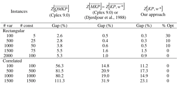
To assess the quality of the four upper bounds we used our lower bound to compute the relative gap (Gap = (upper bound – lower bound)/(lower bound)) since this lower bound was near optimal in most of the instances considered by Djerdjour et al. (1988). Indeed, the simulation results show that our feasible solution was better than the 3 feasible solutions provided by Djerdjour et al. (1988) in 66% of the instances, equal in 33% of them and worse in 1%. Our lower bound is on average 3% higher than the best of the three feasible solutions which are already closed to the optimum (see Djerdjour et al. (1988) for more details). Our lower bound is therefore the best known feasible solution. Our lower and upper bounds as well as the upper bound of Djerdjour et al. were coded in C language. The two other upper bounds (Z

[

QMKP

]

and Z

[ ]

MKP ) were obtained using the commercial software ILOG-Cplex9.0. Simulations were run on a bi-xeon 3.4 Ghz with 4Go of main memory.

Table 1 displays the average deviation of each upper bound to the feasible solution over ten replications of each type of instances. For example, Z

[

QMKP

]

is on average 56.3% higher than our feasible solution over 10 replications of correlated problems with 100 variables and 100 constraints. The last column provides the percentage of instances for which our upper bound corresponds to the optimum value (see Remark 1). It appears that our bound behaves quite well for the rectangular problems for which the overall gap is less than 1.6%. The quality of the upper bound is lower for squared and correlated problems with a gap ranging from 7% to 33%. However, our upper bound significantly outperforms the continuous relaxation of (QMKP) in all cases. Our upper bound is also better than the upper bound Z

[

KP, w*

]

with a maximum improvement of 4.2% for the squared problems (1000,1000). The lowest gap is obtained for rectangular problems as we aggregate less constraints in this type of instances than in the two other classes of problems.

Table 1. Comparison of the quality of the upper bounds

Instances Z

[

QMKP

]

(Cplex 9.0)

[ ] [

MKP ZKP, w*

]

Z = (Cplex 9.0) or (Djerdjour et al., 1988)

[

KP, w*

]

Z Our approach

# var # const Gap (%) Gap (%) Gap (%) % Opt

Rectangular 100 5 2.6 0.5 0.3 30 500 25 2.8 0.4 0.3 10 1000 50 3.8 0.6 0.5 10 1500 75 5.5 1.6 1.5 0 2000 100 5.3 1.0 0.9 0 Correlated 100 100 56.3 14.8 11.2 0 500 500 81.5 20.9 17.3 0

2000 2000 128.8 37.6 33.4 0 Squared 100 100 16.9 9.5 8.2 10 500 500 12.9 7.9 7.5 0 1000 1000 32.2 23.0 21.7 0 1500 1500 37.8 24.6 23.9 0 2000 2000 53.0 36.9 36.2 0

Table 2. Comparison of the CPU times required for each upper bound

# var # const

[

QMKP

]

Z (Cplex 9.0)

[ ]

MKP Z (Cplex 9.0)

[

KP, w*

]

Z (Djerdjour et al.)

[

KP, w*

]

Z Our approach Rectangular 100 5 0.0 0.0 0.3 0.0 500 25 7.5 0.1 10.1 0.1 1000 50 55.3 0.3 41.7 0.4 1500 75 193.1 0.8 100.3 0.8 2000 100 437.9 1.6 183.3 1.8 Correlated 100 100 0.0 0.0 0.0 0.0 500 500 0.0 0.0 0.5 0.0 1000 1000 0.2 0.0 1.5 0.1 1500 1500 0.8 0.1 3.7 0.2 2000 2000 2.2 0.2 7.6 0.4 Squared 100 100 0.0 0.0 0.3 0.0 500 500 7.3 0.1 9.0 0.2 1000 1000 58.2 0.5 37.9 0.5 1500 1500 184.5 1.5 86.6 1.6 2000 2000 421.3 3.4 157.8 3.6

Table 2 displays the CPU time in seconds required to compute the four upper bounds. The most time consuming bound is the continuous relaxation with a maximum of about 8 minutes to solve one of the largest correlated problems. The fastest bound is Z

[ ]

MKP with almost instantaneous results for rectangular problems and an average of 3.4 seconds for the largest squared problems. The time to compute our upper bound deviates at most of 0.2 seconds from the time to obtainZ

[ ]

MKP . Our method can therefore be considered as fast as the previous one. The advantage of computing w* by solving the dual of

( )

MKP rather than using a descent local method as suggested by Djerdjour et al. (1988) strikingly appears: CPU times are sometimes divided by 100.

6. CONCLUSION

In this paper we have designed a method to compute a good upper bound for (QMKP) and we have compared this bound to three other bounds over a large number of instances. The numerical results clearly show that our method provides the best upper bound in a very competitive computational time compared to the linearization which is the quickest method. The proposed upper bound could therefore be utilized in an exact solution method. The computational study also evidenced the good quality of our feasible solution which could consequently be used as an initial solution in a Branch-and-Bound method. It is worth mentioning that the continuous relaxation of (QMKP), although widely used in practice, is not an efficient method from either a qualitatively or a computational standpoint.

A possible way to get a further improvement of the upper bound would be to use a composite relaxation including both a Lagrangean and a surrogate relaxation of the initial problem as suggested by Fréville and Hanafi (2005), who present several methods to solve the 0-1 multidimensional knapsack problem.

7. REFERENCES

1. Bretthauer, K. and Shetty, B. (1996). A projection method for the integer quadratic knapsack problem.Journal

of the Operational Research Society, 47 (3): 457-463.

2. Bretthauer, K. and Shetty, B. (2002a). A pegging algorithm for the nonlinear resource allocation problem.

Computers and Operations Research, 29 (5): 505-527.

3. Bretthauer, K. and Shetty, B. (2002b). The nonlinear knapsack problem – algorithms and applications.

European Journal of Operational Research, 138 (3):459-472.

4. Chu, P.C. and Beasley, J.E. (1998). A Genetic Algorithm for the Multidimensional Knapsack Problem.

Journal of Heuristics, (4): 63-86.

5. Cooper, M. (1981). A survey of methods for pure nonlinear integer programming. Management Science, 27 (3): 353-361.

6. Djerdjour M., Mathur, K. and Salkin, H. (1988). A surrogate-based algorithm for the general quadratic multidimensional knapsack. Operations Research Letters, (7): 253-257.

7. Faaland, B. (1974). An integer programming algorithm for portfolio selection. Management Science, 20 (10): 1376-1384.

8. Fréville, A. and Hanafi, S. (2005). The multidimensional 0-1 Knapsack Problem-Bounds and Computational Aspects. Annals of Operations Research, (139): 195-227.

9. Fréville, A. and Plateau, G. (1986). Heuristics and Reduction Methods for Multiple Constraints 0-1 Linear Programming Problems. European Journal of Operational Research, (24): 206-215.

10. Glover, F. (1965). A Multiphase-Dual Algorithm for the Zero-One Integer Programming Problem.

Operations Research, (13): 879-919.

11. Glover, F. (1975). Improved linear programming formulations of nonlinear integer problems. Management

Science, 22 (4): 455-460.

12. Körner, F. (1985). Integer quadratic programming. European Journal of Operational Research, 19 (2): 268-273.

14. Markowitz, H.M. (1952). Portfolio Selection. Journal of Finance, 7 (1): 77-91.

15. Martello, S. and Toth, P. (2003). An exact algorithm for the two-constaint 0-1 knapsack problem.

Operations Research, 51 (5):826-835.

16. Martello, S. and Toth, P. (1990). Knapsack Problems: algorithms and computer implementations. John Wiley & Sons, Inc. New York, NY, USA.

17. Mathur, K., Salkin, H. and Morito, S. (1983). A branch and search algorithm for a class of nonlinear knapsack problems. Operations Research Letters, 2 (4): 155-160.