HAL Id: hal-00619855
https://hal-upec-upem.archives-ouvertes.fr/hal-00619855
Submitted on 6 Oct 2011
HAL is a multi-disciplinary open access
archive for the deposit and dissemination of
sci-entific research documents, whether they are
pub-lished or not. The documents may come from
teaching and research institutions in France or
abroad, or from public or private research centers.
L’archive ouverte pluridisciplinaire HAL, est
destinée au dépôt et à la diffusion de documents
scientifiques de niveau recherche, publiés ou non,
émanant des établissements d’enseignement et de
recherche français ou étrangers, des laboratoires
publics ou privés.
Conjugacy and Equivalence of Weighted Automata and
Functional Transducers
Marie-Pierre Béal, Sylvain Lombardy, Jacques Sakarovitch
To cite this version:
Marie-Pierre Béal, Sylvain Lombardy, Jacques Sakarovitch. Conjugacy and Equivalence of Weighted
Automata and Functional Transducers. 1st International Computer Science Symposium in Russia
(CSR 2006), Jun 2006, St. Petersburg, Russia. pp.58-69. �hal-00619855�
Conjugacy and equivalence of
weighted automata and functional transducers
Marie-Pierre B´eal1, Sylvain Lombardy2, and Jacques Sakarovitch3 1
Institut Gaspard-Monge, Universit´e Marne-la-Vall´ee.
2
LIAFA, Universit´e Paris 7.
3
LTCI, CNRS / Ecole Nationale Sup´erieure des T´el´ecommunications. (UMR 5141) [email protected] [email protected] [email protected]
Abstract. We show that two equivalent K-automata are conjugate to a third one, when K is equal to B, N, Z, or any (skew) field and that the same holds true for functional tranducers as well.
extended abstract
1
Presentation of the results
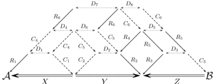
In a recent paper ([1]), we have studied the equivalence of Z-automata. This equivalence is known to be decidable (with polynomial complexity) for more than forty years but we showed there two results that give more structural information on two equivalent Z-automata. We first proved that two equivalent Z-automata are related by a series of three conjugacies — we shall define conjugacy later in the paper — and then that every conjugacy relation can be decomposed into a sequence of three operations: state (out-)splitting (also known as covering), circulation of coefficients, and state (in-)merging (also known as co-covering). Altogether, we reached a decomposition of any equivalence between Z-automata as the one described at Figure 1 [Conjugacy is represented by double-line arrows, coverings by simple solid arrows, co-coverings by simple dashed arrows, and circulation by simple dotted arrows].
X Y Z C2 C3 C4 C4 C5 C5 C6 C6 C1 R1 R2 R3 R4 R5 R5 R6 R6 D1 D2 D3 D4 D6 D5 D7 D8
A
B
Fig. 1.Structural decomposition of the equivalence of two Z-automata.
At the end of our ICALP paper we mentioned two problems open by the gap between these results and those that were formerly known. First, whether three
conjugacies are necessary (in general), and, if yes, whether it is decidable when two conjugacies suffice. Second, whether, in the case of N-automata, the whole chain of conjugacies could be always realized with transfer matrices in N and, if not, whether it is decidable when this property holds.
We answer these two questions here. By means of techniques different from the ones that where developed in [1], we show that two conjugacies always suffice and that this property holds not only for Z-automata but also for N-automata and other families of automata as stated by the following.
Theorem 1. Let K be B, N, Z, or any (skew) field. Two K-automata are equiv-alent if and only if there exists a third K-automaton that is conjugate to both of them.
Moreover, an analoguous result holds for functional transducers as well. Theorem 2. Two functional transducers are equivalent if and only if there ex-ists a third functional transducer that is conjugate to both of them
Together with these results on conjugacy, we extend the decomposition of conjugacy by means of covering, co-covering and “circulation” as follow (we shall define covering and co-covering more precisely at Section 3). We state the first one for sake of completeness.
Theorem 3 ([1]). Let K be a field F or the ring Z and let A and B be two K-automata. We have A =⇒ B if and only if there exists two K-automata CX and D and a circulation matrix D such that C is a co-K-covering of A, D a K-covering of B and C=⇒ D .D
Theorem 4. Let K be the semiring N or the Boolean semiring B and let A and B be two trim K-automata. We have A=⇒ B if and only if there exists aX K-automaton C that is a co-K-covering of A and a K-covering of B.
Theorem 5. Let A and B be two trim functional transducers. We have A=⇒X B if and only if there exists two (functional) transducers C and D and a diagonal matrix of words D such that C is a co-covering of A, D a covering of B and
C=⇒ D .D
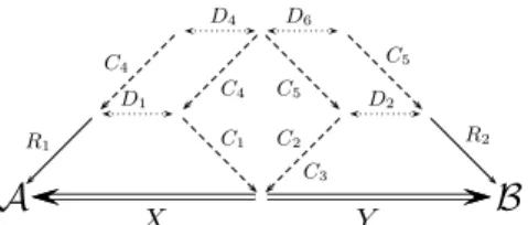
In other words, Figure 1 can be replaced by Figure 2 where A and B are taken in any family considered in Theorems 1 and 2.
The present result on conjugacy is both stronger and broader than the pre-ceeding ones. Stronger as the number of conjugacies is reduced from three to two, broader as the result apply not only to Z-automata (indeed to automata with multiplicity in an Euclidean domain) but to a much larger family of automata. It answers in particular to what was a long standing problem for the authors: is it possible to transform an N-automaton into any other equivalent one using only state splitting and state merging? The answer is thus positive, and the chain of operations is rather short. The benefit brought by the change from Z into N is well illustrated by the following consequence.
X Y C2 C3 C4 C4 C5 C5 C1 R1 R2 D1 D2 D4 D6
A
B
Fig. 2.Structural decomposition of the equivalence of two K-automata.
Theorem 6. If two regular languages have the same generating function (i.e. the numbers of words of every length is the same in both languages) then there exists a letter-to-letter rational function that realizes a bijection between the two languages.
2
Conjugacy and covering of automata
A finite automaton A over an alphabet A with multiplicity in a semiring K, or K-automaton for short, can be written in a compact way as A = hI, E, T i where E is a square matrix of finite dimension Q whose entries are linear combinations (with coefficients in K) of letters in A and where I and T are two vectors — respectively row vector and column vector — with entries in K as well. We can view each entry Ep,q as the label of a unique arc which goes from state p to
state q in the graph whose set of vertices is Q (if Ep,q = 0K, we consider that
there is no arc from p and q).
The behaviour of A, denoted |||A|||, is the series such that the coefficient of a word w is the coefficient of w in I E|w|T . It is part of Kleene-Sch¨utzenberger Theorem that every K-rational series is the behaviour of a K-automaton of the form we have just defined. For missing definitions, we refer to [4, 2, 10].
2.1 Conjugacy
Definition 1. A K-automaton A = hI, E, T i is conjugate to a K-automaton B = hJ, F, U i if there exists a matrix X with entries in K such that
I X = J, E X = X F, and T = X U.
The matrix X is the transfer matrix of the conjugacy and we write A=⇒ B .X Remark that in spite of the idea conveyed by the terminology, the conjugacy relation is not an equivalence but a preorder relation. Suppose that A =⇒ CX holds; if C =⇒ B then AY =⇒ B , but if BXY =⇒ C then A is not necessarilyY conjugate to B, and we write A=⇒ CX ⇐= B or even AY =⇒X ⇐= B .Y
This being well understood, we shall speak of “conjugate automata” when the orientation does not matter. For instance, we state that, obviously, two conjugate automata are equivalent (i.e. have the same behaviour).
2.2 Covering
The standard notion of morphisms of automata — which consists in merg-ing states and does not tell enough on transitions — is not well-suited to K-automata. Hence the definitions of K-coverings and co-K-coverings. These have probably stated independently a number of times. We describe them here in terms of conjugacy. A definition closer to the classical morphisms could be given and then the definitions below become propositions (cf. [1, 10]).
Let ϕ : Q → R be a surjective map and Hϕ the Q × R-matrix where the
(q, r) entry is 1 if ϕ(q) = r, 0 otherwise. Since ϕ is a map, each row of Hϕ
contains exactly one 1 and since ϕ is surjective, each column of Hϕ contains at
least one 1. Such a matrix is called an amalgamation matrix ([6, Def. 8.2.4]). Let A and B be two K-automata of dimension Q and R respectively. We say that B is a K-quotient of A and conversely that A is a K-covering of B if there exists a surjective map ϕ : Q → R such that A is conjugate to B by Hϕ
The notion of K-quotient is lateralized since the conjugacy relation is not symmetric. Somehow, it is the price we pay for extending the notion of morphism to K-automata. Therefore the dual notions co-K-quotient and co-K-covering are defined in a natural way. We say that B is a co-K-quotient of A and conversely that A is a co-K-covering of B if there exists a surjective map ϕ : Q → R such that B is conjugate to A by tH
ϕ.
We also write ϕ : A → B and call ϕ, by way of metonymy, a K-covering, or a co-K-covering from A onto B.
3
The joint reduction
The proof of Theorems 1 and 2 relies on the idea of joint reduction which is defined by means of the notion of representation.
An automaton A = hI, E, T i of dimension Q can equivalently be described as the representation A = (I, µ, T ) where µ : A∗ → KQ×Q is the morphism
defined by the equality
E =X
a∈A
µ(a) a .
This equality makes sense since the entries of E are assumed to be linear combi-nations of letters of A with coefficients in K. And the coefficient of any word w in the series |||A||| is I µ(w) T .
The set of vectors {I µ(w) | w ∈ A∗} (row vectors of dimension Q), that is,
the phase space of A, plays a key role in the study of A, as exemplifyed by the following two contrasting cases.
If A is a Boolean automaton, this set of vectors (each vector represents a subset of the dimension Q) is finite and makes up the states of the determinized automaton D of A (by the subset construction). Moreover, if we form the ma-trix X whose rows are the states of D, then D is conjugate to A by X.
If A is a K-automaton with K a field, the left reduction of A — recalled with more detail below — consists in choosing a prefix-closed set P of words such
that the vectors {I µ(p) | p ∈ P } is a basis of the vector space generated by {I µ(w) | w ∈ A∗} (cf. [2]). Moreover the (left-)reduced automaton is conjugate
to A by the matrix X whose rows are the vectors {I µ(p) | p ∈ P } .
Let now A = (I, µ, T ) and B = (I0, κ, T0) be two K-automata of
dimen-sion Q and R respectively. We consider the union of A and B and thus the vectors [I µ(w)|I0κ(w)] of dimension Q ∪ R . These vectors, for w in A∗,
gener-ate a K-module W . The (left) joint reduction of A and B consists in computing — when it is possible — a finite set G of vectors [x|y] which generate the same K-module W . Then the matrix M whose rows are these vectors [x|y] provides in some sense a K-automaton C which is conjugate to both A and B with the transfer matrices X and Y respectively, where X and Y are the ‘left’ and ‘right’ parts of the matrix M respectively.
In every case listed in the above Theorems 1 and 2, and which we consider now, the finite set G is effectively computable.
3.1 Joint reduction in fields
Let K be a field and let A = (I, µ, T ) be a K-automaton of dimension n. The reduction algorithm for K-automata is split into two dual parts. The first part consists in computing a prefix-closed subset P of A∗ such that the
set G = {I µ(w) | w ∈ P } is free and, for every letter a, and every word in P , I µ(wa) is lineary dependant from G. The set G has at most n elements and an automaton C = (J, κ, U ), whose states are the elements of G, is defined by:
Jx=
(
1 if x = I ,
0 otherwise , ∀x ∈ G, Ux= xT , ∀a, ∃!κ(a), ∀x ∈ G, xµ(a) = X
y∈G
κ(a)x,yy .
This can be viewed as a change of basis: the set G generates the smallest subspace of Kn that contains every I µ(w) and if G is completed into a basis B, after
changing the canonical basis by B and projection, one gets the automaton C. Finally, if M is the matrix whose rows are the elements of G, it holds C=⇒ A.M The second part is similar and consists in computing a basis of the subspace of K|G| generated by the vectors κ(w) U . It is a nice result (by Sch¨utzenberger)
that after these two semi-reductions, the outcome is a K-automaton of smallest dimension that is equivalent to A.
We focus here on the first part which we call left reduction. Let A = (I, µ, T ) and B = (I0, µ0, T0) be two equivalent K-automata and let C
0 = (J, κ, U ) be
the automaton obtained by left reduction of A + B. The automaton A + B has a representation equal to ([I|I0], diag(µ, µ0), [T |T0]), where [I|I0] is obtained by horizontally joining the row vectors I and I0, [T |T0] by vertically stacking the
column vectors T and T0, and for every letter a, [diag(µ|µ0)](a) is the matrix
The automaton C0is conjugate to A + B by the matrix [X|Y ], in which every
row has the form [I µ(w)|I0µ0(w)] where w is a word. It holds:
J [X|Y ] = [I|I0], ∀a, κ(a) [X|Y ] = [X|Y ] (diag(µ|µ0))(a), U = [X|Y ] [T |T0] As A and B are equivalent, X T = Y T0 and thus U = 2 X T = 2 Y T0. Let
C = hJ, κ, U/2i; it immediatly comes C =⇒ A and CX =⇒ B .Y 3.2 Joint reduction in Z
The result and the algorithm are basically the same as the previous ones if the multiplicity semiring is Z. As in vector spaces, there is a dimension theory in the free Z-modules and it is still possible to compute a basis G of the submodule of Zn generated by the vectors I µ(w). However, this basis does not correspond
any more to a prefix-closed set of words. and the algorithm to compute it is explained in [1].
3.3 Joint reduction in N
There is no dimension theory in the N-modules and thus no reduction algorithm for N-automata similar to the previous ones.
However, given A + B our aim is not the reduction itself but the computation of a set G of vectors with the 3 properties: for every z = [x|y] in G, x T = y T0 holds, the N-module hhhG iii generated by G is closed under multiplication
by (diag(µ|µ0))(a), for every letter a (which is important to effectively build
the automaton C), and finally G is finite. It can be noted that in the preceeding algorithms, the freeness of the generating set G is used only to garantee finiteness. An algorithm that compute such a G for N-automata can be roughly sketched as follows.
Start from G = {[I|I0]}. While hhhG iii is not closed under (diag(µ|µ0))(a), take
z = [x|y] in G (diag(µ|µ0))(a) \ hhhG iii add z to G, and reduce G. The reduction
goes as follow: while G contains z and z0 such that z < z0 (in the product order
of NQ∪R) replace z0 by z0− z. This algorithm ends since at every step, either
the size of vectors of G decreases or the size of G increases. The size of vectors cannot decrease infinitely and as vectors of G are pairwise incomparable (after the reduction step), G has only a finite number of elements.
The outcome of this algorithm is not canonically associated to A and B and even its size (in contrast to what happens with fields) may depend on the order in which comparable pairs are considered during the reduction step. Yet, an automaton C whose states are the elements of G is built as the previous cases. 3.4 Joint reduction in B
In B, as in many semirings that cannot be embedded in rings, there is no sub-traction. Therefore it is quite difficult to reduce vectors [I µ(w)|I0µ0(w)] to find
vectors [I µ(w)|I0µ0(w)] . The automaton C obtained from this set is nothing
else that the determinised automaton of A ∪ B. For the same reason as above, this automaton is conjugate both to A and B.
3.5 Joint reduction of functional transducers
With transducers, difficulties of automata with multiplicities and Boolean au-tomata meet. On the one hand, if T = (I, µ, T ), the set {Iµ(w) | w ∈ A∗} may
be infinite and, in the other hand, as in the Boolean case, the substraction is not allowed in the semiring of multiplicities that can be associated to them.
If the transducers A and B were sequentialisable, it would be sufficient to consider the sequentialised transducer of their union that would be conjugate to each of them. The idea of the sequentialisation (cf. [3, 7]) is to compute a (finite) set of vectors of words, each vector being the information that can not be output and that is necessary for further computation.
On general functional transducers, this algorithm does not always end. We present now a pseudo-sequentialisation, that stops on any functional transducer. This algorithm allows to split vectors of words when their components are dif-ferent enough, which induces non deterministic transitions.
We describe first this algorithm on one functional transducer and then explain how to use it for the joint reduction.
Definition 2. Let k be a positive integer and X be a se of words. Two words u and v of A∗ are k-related in X, if there exists a finite sequence w
0, ..., wn of
words such that u = w0, v = wn, for every i in [1; n], d(wi−1, wi) 6 k and there
exists i in [1; n] such that wi is a prefix of u and v. The set X is k-related if
every pair of its elements is k-related in X. The k-relation is an equivalence on X.
Definition 3. Let α be a vector of words. The k-decomposition of α is the small-est set of vectors Dk(α) such that, for every β ∈ Dk(α) the set of components
of β is k-related and α =P
β∈Dk(α)β.
Obviously, the vectors of Dk(α) have disjoint supports. We shall applies this
decomposition to vectors of words and then reduce them with respect to their greatest common prefix; this second step is exactly the same as in the classical sequentialisation algorithm.
Definition 4. Let α be a vector of words. We denote α the greatest common◦ prefix of non zero components of α and α]=α◦−1α.
Definition 5. Let T = (I, µ, T ) be a functional transducer and let k be non negative integer The k-pseudo-sequentialised transducer S of T is defined by: – for every β in Dk(I), β] is an initial state with initial weight
◦
β;
– for every state α, for every letter a, for every β in Dk(αµ(a)), there is a
transition labeled by a with outputβ from α to β◦ ].
Proposition 1. For k, the k-pseudo-sequentialised transducer S of a functional transducer T is a finite transducer that is conjugate to T .
The transducer S is finite since the components of its states (that are vectors) are bounded by k.
If the k-pseudo-sequentialisation is applied to the union of two equivalent functional transducers A = (I, µ, T ) and B = (I0, µ0, T0), it gives a transducer
C which is conjugate to A ∪ B with a matrix M = [X|Y ], but, in general, this transducer is not conjugate to A with X and to B with Y . Actually, if k is too small, there may be rows [x|y] of M such that xT 6= yT0.
Let k be equal to n2L, where n is the maximum of dimensions of A and B
and L is the longest output of transitions or terminal functions of A and B. In this case, the k-pseudo-sequentialised transducer is unambiguous, which implies that xT = yT0for every state [x|y] of C. Therefore, the transducer C is conjugate
both to A and B.
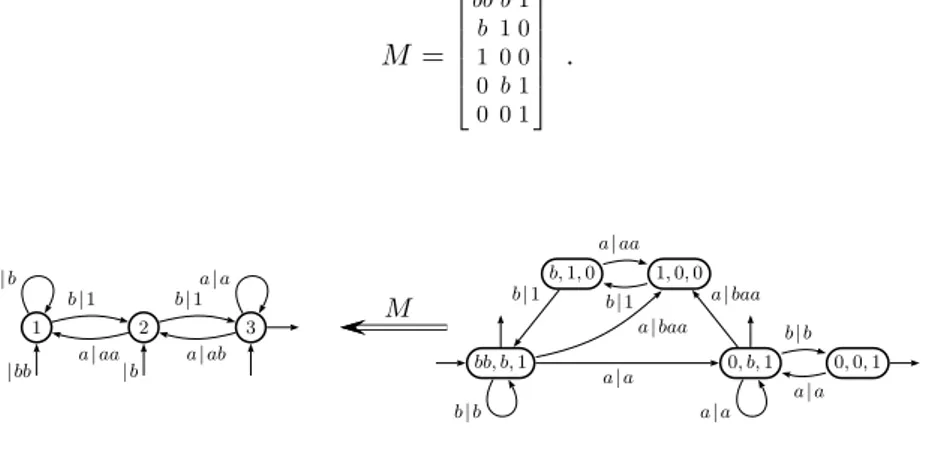
Example 1. Figure 3 shows the transducer T1and its k-pseudo-sequentialised S1
(the result is the same with any positive k), where T1 is the (left) transducer
that replaces systematically factors abb by baa when reading words from right to left; T1 is thus co-sequential, that is, input co-deterministic (cf. [10]). The
transducer S1 is conjugate to T1 with the transfer matrix M :
M = bb b 1 b 1 0 1 0 0 0 b 1 0 0 1 . 1 2 3 | bb | b b| b a| a b| 1 a| aa b| 1 a| ab bb, b,1 b,1, 0 1, 0, 0 0, b, 1 0, 0, 1 b| b a| a a| baa a| a a| aa b| 1 b| 1 a| baa b| b a| a M
Fig. 3.The transducers T1and S1
The above list may lead to think that a joint reduction procedure may be found for any semiring. This is certainly not the case and the tropical semirings for instance, or the non functional transducers, are not likely to admit a joint reduction procedure.
4
From conjugacy to coverings
4.1 The case of fields and integers
We have proved Theorem 3 in [1]. Actually, every matrix M can be decomposed in a product H D K, where tH and K are amalgamation matrices and D is a
diagonal matrix whose entries are invertible. If K is a field, the dimension of D is the number of non zero entries of M , and if K = Z, as the only invertible elements are 1 and −1, every non zero element has to be decomposed in a sum of ±1 and the dimension of D is the sum of the absolute values of the entries of M .
The proof consists then in proving that there exist automata C and D such that A =⇒ CH =⇒ DD =⇒ B. The construction of C and D amounts to fill inK blocks of their transition matrix knowing the sum of the rows and the columns. For natural integers, the proof is exactly the same. The unique invertible element of N is 1, thus D is the identity matrix. However, to get the expected form, the matrix M must have no zero row or column.4 This is ensured by the
assumption that A and B are trim. 4.2 The Boolean case
Let A = (I, µ, T ) and B = (J, κ, U ) be two trim automata such that there exists a n × m Boolean matrix X that verifies A=⇒ B.X
Let k be the number of non zero entries of matrix X. We define ϕ : [1; k] → [1; n] and ψ : [1; k] → [1; m], such that xϕ(i),ψ(i) is the i-th non zero entry of
X. Let Hϕ and Hψ be the matrices associated to these applications. It holds
X = tH
ϕ Hψ. We define C = (K, ζ, V ) with dimension k by:
K = I tHϕ , V = HψU ,
∀(p, q) ∈ [1; k]2, ζ(a)p,q= µ(a)ϕ(p),ϕ(q)∧ κ(a)ψ(p),ψ(q) .
It is then easy to check that C
tH ϕ
=⇒ A and C =⇒ B, which means that C is aHψ co-B-covering of A and a B-covering of B.
In the case were A is the determinised automaton of B (which arises if one applies the algorithm given in the previous section), the automaton built in this way is the Sch¨utzenberger covering of B, a construction that appears naturally in a number of problems for automata with multiplicity (cf. [5, 9, 10]).
4.3 The functional transducer case
Let A = (I, µ, T ) and B = (J, κ, U ) be two trim functional transducers and let X be a n × m matrix of words such that A=⇒ B. Let k be the number of nonX zero entries of X. The matrix X can be decomposed into H D K, where H and K are Boolean matrices and D is a diagonal matrix of words of dimension k.
4
This diagonal matrix corresponds to a circulation of words. Actually, in the framework of transducers, the circulation of words is a well-known operation that is needed for instance in the minimisation of sequential transducers. This operation can be related to the circulation of invertible elements for fields if we consider words as elements of the free group.
We want to prove that there exists A0 = (I0, µ0, T0) and B0 = (J0, κ0, U0)
such that A =⇒ AH 0 =⇒ BD 0 =⇒ B. We set IK 0 = I H, J0 = I0D, U0 = K U and
T0= D U0.
For every letter a, there exists a matrix ζ(a) such that H ζ(a) = µ(a) H D and ζ(a) K = D K κ(a). As H and K are Boolean matrices, ζ(a) can be factorised in µ0(a) D and D κ0(a), which gives the solutions.
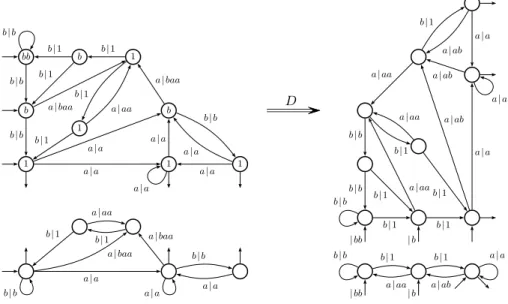
| bb | b b| b b| 1 a| a a| aa b| 1 a| ab | bb | b a| aa a| ab a| a a| aa a| ab a| a a| ab a| a b| b b| 1 b| 1 b| b b| 1 b| 1 b| b b| 1 a| aa b| 1 b| b a| a a| baa a| a a| aa b| 1 b| 1 a| baa b| b a| a bb b 1 b 1 1 b 1 1 a| baa a| a a| a a| baa a| a a| a a| a a| a b| b b| b b| b b| 1 b| 1 b| 1 b| 1 b| 1 a| aa b| b D
Fig. 4.The instance of Theorem 5 for S1 and T1
5
An application
Theorem 6 is a striking consequence of the strengthening of our conjugacy result of [1] and answers a question on automatic structures.
Let A and B be two (Boolean) unambiguous automata the languages L and K respectively and suppose that L and K have the same generating functions. It amounts to say that if we forget the labels in A and B (and replace them all by the same letter x) we have two equivalent N-automata A0and B0: the coefficient
of xn in |||A0||| and thus in |||B0||| is the number of words of length n in L and thus
By Theorem 1, A0 and B0 are both conjugate to a same N-automaton C0 (on
x∗). By Theorem 4 there exist D0 and E0 such that D0 is a co-N-covering of C0
and a N-covering of A0 and E0 is a co-N-covering of C0 and a N-covering of B0. By a diamond lemma ([1, Proposition 6]) there exists a N-automaton T0 (on x∗)
which is a co-N-covering of D0 and of E0.
Every transition of T0 is mapped, via the co-N-coverings and the N-coverings
onto a transition of A0 and onto a transition of B0. But these are transitions of
A and B and every transition of T0 may thus be labelled by a pair of letters
(one coming from A and one coming from B) and hence turned into a letter-to-letter transducer T . As the projection on each component gives an unambiguous automaton, T realises a bijective function.
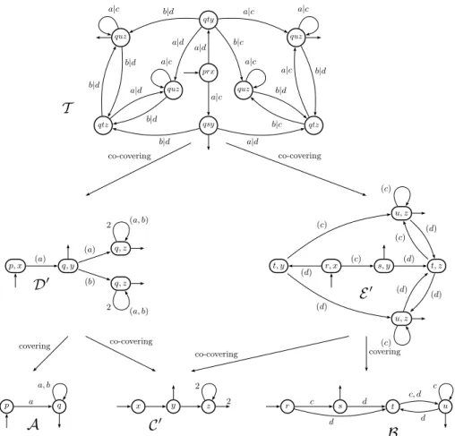
Remark 1. Theorem 6 bears some similarity with an old result by Maurer and Nivat (cf. [8]) on rational bijections. It is indeed completely different: it is more restricted in the sense it applies only to languages with the same generating functions whereas Maurer and Nivat considered bijections between languages with ‘comparable’ growth functions, and it is much more precise in the sense that the transducer which realizes the bijection is letter-to-letter. It is this last property that makes the result interesting for the study of automatic structures. Figure 5 shows the construction for the two languages L = a(a + b)∗ and
K = (c + dc + dd)∗rcc(c + d)∗ recognized by their minimal deterministic (and
thus unambiguous) automata A and B.
References
1. B´eal, M.-P., Lombardy, S. and Sakarovitch, J. On the equivalence of Z-automata. Proc. ICALP’05 , LNCS 3580, Springer (2005) 397–409.
2. Berstel, J., and Reutenauer, Ch. Rational Series and their Languages. Springer, 1988.
3. Choffrut, Ch. Une caractrisation des fonctions squentielles et des fonctions sous-squentielles en tant que relations rationnelles. Theoret. Comput. Sci. 5 (1977), 325–337.
4. Eilenberg, S. Automata, Languages, and Machines. Vol. A. Academic Press, 1974.
5. Klimann, I., Lombardy, S., Mairesse J., and Prieur, Ch. Deciding unambi-guity and sequentiality from a finitely ambiguous max-plus automaton. Theoret. Comput. Sci. 327 (2004), 349–373.
6. Lind, D., and Marcus, B. An Introduction to Symbolic Dynamics and Coding. Cambridge University Press, 1995.
7. Lombardy, S. and Sakarovitch, J. Sequential ?. Theoret. Comput. Sci., to appear.
8. Maurer, H., and Nivat, M. Rational Bijection of Rational Sets. Acta Informatica 13 (1980) 365–378.
9. Sakarovitch, J., A construction on automata that has remained hidden. Theoret. Computer Sci. 204 (1998), 205–231.
10. Sakarovitch, J., El´ements de th´eorie des automates, Vuibert, 2003. English translation, Cambridge Universit Press, to appear.
p q