HAL Id: hal-00879825
https://hal.inria.fr/hal-00879825
Submitted on 5 Nov 2013
HAL is a multi-disciplinary open access
archive for the deposit and dissemination of
sci-entific research documents, whether they are
pub-lished or not. The documents may come from
teaching and research institutions in France or
abroad, or from public or private research centers.
L’archive ouverte pluridisciplinaire HAL, est
destinée au dépôt et à la diffusion de documents
scientifiques de niveau recherche, publiés ou non,
émanant des établissements d’enseignement et de
recherche français ou étrangers, des laboratoires
publics ou privés.
Regular Set of Representatives for Time-Constrained
MSC Graphs
Sundararaman Akshay, Blaise Genest, Loïc Hélouët, Shaofa Yang
To cite this version:
Sundararaman Akshay, Blaise Genest, Loïc Hélouët, Shaofa Yang. Regular Set of Representatives for
Time-Constrained MSC Graphs. Information Processing Letters, Elsevier, 2012, 112 (14-15),
pp.592-598. �hal-00879825�
Regular Set of Representatives for Time-Constrained MSC Graphs
I S. Akshaya, Blaise Genesta,b, Lo¨ıc H´elou¨eta, Shaofa YangcaIRISA, ENS Cachan Bretagne - CNRS - INRIA, Rennes, France bCNRS, UMI IPAL joint with NUS and A*STAR/I2R, Singapore
cSIAT, Chinese Academy of Sciences, China
Abstract
Systems involving both time and concurrency are notoriously difficult to analyze. Existing decidability results apply when clocks on different processes cannot be compared or when the set of timed executions is regular. We prove new decidability results for timed concurrent systems, requiring neither restriction. We consider the formalism of time-constrained MSC-graphs (TC-MSC graphs for short) introduced in [1], and study if the set of timed executions generated by a TC-MSC graph is empty. This emptiness problem is known to be undecidable in general [9]. Our approach consists of finding a regular set R of representative timed executions, i.e., such that every timed execution of the system has an equivalent, up to commutation, timed execution in R. This allows us to solve the emptiness problem under the assumption that the TC-MSC graph is prohibited from (1) forcing any basic scenario to take an arbitrarily long time to complete and (2) enforcing unboundedly many events to occur within one unit of time.
Keywords: timed automata, partial order languages, MSC graphs, set of representatives
1. Introduction
In a distributed system, several processes in-teract to implement a collection of global behav-iors. These processes are often equipped with tim-ing information and protocol specifications include timing requirements for messages and descriptions of how to recover from timeouts. Thus, a sys-tem designer has to deal with situations where time and concurrency influence each other. One way to describe these interactions is through sce-narios, formalized using Message Sequence Charts (MSCs) [12]. The timing information is captured by adding timing constraints between pairs of events, yielding time-constrained MSCs (TC-MSCs). Fur-ther, infinite collections of MSCs can be modelled using High-level Message Sequence Charts, or more basic forms called MSC-graphs: directed graphs whose nodes are labelled by MSCs. MSC-graphs can be generalized to time-constrained MSC graphs IThis work was supported by the DST INRIA associated
team, CNRS PEPS AABS, and ANR IMPRO project.
Email addresses: akshay@irisa.fr (S. Akshay),
blaise.genest@irisa.fr(Blaise Genest), loic.helouet@irisa.fr(Lo¨ıc H´elou¨et), sf.yang@siat.ac.cn(Shaofa Yang)
(TC-MSC graphs)[9], whose nodes are labelled by TC-MSCs and edges have additional timing con-straints. In this paper, we focus on decidability results for the analysis of TC-MSC graphs.
Obtaining decidability in the presence of both time and concurrency is a challenging issue. Even the simple yet fundamental question of checking if there exists a timed execution of a TC-MSC graph consistent with all the constraints is undecidable in general [9]. This is the emptiness problem, which in the case of (sequential) timed automata is known to be decidable [3]. Extending such results to dis-tributed systems has been done only in two par-ticular and limited settings. In [13, 8], clocks are local to a process. But then, one cannot specify time taken by a communication (message or syn-chronisation). This limitation makes the specifica-tion formalism very weak. The second setting can relate clocks from different processes and specify how long a communication can take [1, 2, 6, 7]. However, they restrict the concurrency in a struc-tural way, for instance by considering only locally synchronized ([15, 4, 11]) MSC-graphs (in [1, 2]) or only safe Petri Nets (in [6, 7]). This forces the set of timed executions defined by the specification to
be (timed) regular, which is a significant restriction in a concurrent setting where even simple examples may not be regular (e.g., the producer-consumer protocol).
In this paper, we propose a first decidability re-sult for (globally) timed concurrent systems hav-ing a possibly non-regular set of behaviors. More specifically, we tackle the emptiness problem for TC-MSC graphs (which is undecidable in gen-eral [9]) by coming up with mild restrictions which are practically motivated and yet sufficient to prove decidability. Our technique to obtain decidability is to use a regular set of representatives. A set of representatives is a subset of executions such that every execution of the system has an equivalent ex-ecution (up to commutation) in this subset. This technique has been used previously in untimed set-tings [14, 10] and with the particular set of exis-tentially bounded executions [10] as the regular set of representatives. In Section 3, it is formalized as a general technique on timed languages and ap-plied to the set of well-behaved timed executions, i.e., timed executions where two events from the same scenario do not occur at dates that are arbi-trarily apart (non-drifting) and only a limited num-ber of events can occur in a unit of time (non-Zeno). We state our main theorems in Section 4: the set of well-behaved timed executions of a TC-MSC graph is regular, and it is a set of representatives under the assumption that the TC-MSC graph is well-formed. Together, these imply that the empti-ness problem is decidable for well-formed TC-MSC graphs. Intuitively, being well-formed prohibits specifications in which (1) events from the same scenario are forced to occur arbitrarily apart from each other (drifting), which is undesirable as it goes against the MSC-graph design, and (2) an un-bounded number of events are forced to happen within one unit of time, which is unimplementable. Proofs are detailed in Section 5. Regularity of the set of well-behaved executions exploits the fact that if node x appears sufficiently before node y in a path, then all events of x must occur before any event of y in any well-behaved execution of this path. Proving representativity for a well-formed TC-MSC graph is not trivial, as for each execution, we need to find a representative which is both non-drifting and has a limited number of events per unit of time, while being well-formed guarantees only the existence of two representatives, one of each kind. Further discussion regarding significance and practicality of our assumptions can be found in [17].
2. Time-Constrained MSC graphs
We fix a finite non-empty set of processes P that communicate through messages via reliable FIFO channels. For p, q ∈ P, the communication alpha-bet is Σ = {p!q, p?q | p 6= q} where the send action p!q denotes a message sent from process p to q and the receive action q?p denotes a message received by process q from p. Let N denote the set of natural numbers and I(N) denote the set of open and closed intervals whose end points are in N, plus the inter-vals of the form [c, ∞), (c, ∞), where c ∈ N. We shall use intervals in I(N) to constrain the lower and upper bounds on the difference of occurrence times of events in a scenario. We remark that in what follows, intervals involving non-negative ra-tionals can be easily simulated by scaling them to integers. We adopt the basic definitions from [1]. Definition 2.1. A time-constrained message se-quence chart (TC-MSC) over P and Σ is a tuple T = (E, (<p)p∈P, λ, µ, δ) where E is a finite
non-empty set of events; λ : E → Σ labels each event with an action type in Σ such that:
(i) Each <p⊆ Ep × Ep is a total order, where
Ep = λ−1({p} × {!, ?} × P). Members of Ep
are termed p-events.
(ii) The message relation µ is a bijection from Esend = λ−1(P × {!} × P) (send events) to
Erecv = λ−1(P × {?} × P) (receive events).
For any e, f with µ(e) = f , for some p, q, we have λ(e) = p!q and λ(f ) = q?p. For each e, e′
with λ(e) = λ(e′) = p!q for some p, q ∈ P, we
have e <pe′ iff µ(e) <q µ(e′). (FIFO)
(iii) Writing < for the transitive closure of (Sp∈P<p) ∪ µ, the time constraint labelling
function δ associates an interval in I(N) to each pair of events (e, f ) ∈ E × E with e < f . With a slight abuse of notation, we write a TC-MSC as T = (E, <, λ, µ, δ), with < as above. A linearization of T is a sequence σ = a1. . . aℓ over
Σ∗, where ℓ = |E| and such that E can be enumer-ated as e1. . . eℓwith ai= λ(ei), and ei< ejimplies
i < j for any i, j in {1, . . . , ℓ}. Note that due to the FIFO condition (see Condition (ii) in the defi-nition above), the enumeration e1. . . eℓis uniquely
determined by a1. . . aℓ. A TC-MSC T defines a
col-lection of linearizations augmented with occurrence times such that the relative delay between each pair of causally ordered events falls within the interval 2
n1 ⇒ p q [0, 3] n2 p r n3 q r ([0, 2],⊥,⊥) (⊥,(2, 3],⊥) T1 p q r [0, 3] [0, 2] T2 p q r [0, 3] [0, 3] [0, 3] [0, 2] (2, 3] (2, 3]
Figure 1: A TC-MSC graph G1and two TC-MSCs it generates dictated by δ. To avoid confusion, we shall term
occurrence times as dates: A timed execution w of T is a sequence (a1, d1) . . . (aℓ, dℓ), where a1. . . aℓis
a linearization of T , each date di is a non-negative
real for i = 1, . . . , ℓ, and d1≤ . . . ≤ dℓ. Let e1. . . eℓ
be the enumeration corresponding to the lineariza-tion a1. . . aℓ. Then ei< ej implies dj− di is in the
interval δ(ei, ej).
To describe infinite collections of TC-MSCs, we use TC-MSC graphs:
Definition 2.2. Let T be a finite non-empty set of TC-MSCs. A TC-MSC graph over T is a tuple G = (N, −→, nini, Nfin, Λ, ∆) where N is a finite set of
nodes, −→⊆ N × N a transition relation, nini ∈ N
the initial node, Nfin ⊆ N the subset of final nodes,
and Λ : N → T labels each node with a TC-MSC from T . Further, the mapping ∆ associates each transition (n, n′) in −→ with a P-indexed family of
intervals in I(N), such that if either n or n′ has no
p-event, then the p-component of ∆(n, n′) is [0, ∞).
For each p, we write ∆p(n, n′) for the p-th
com-ponent of ∆(n, n′). The interval ∆
p(n, n′) specifies
the range of relative delay on p when moving from n to n′. We write ⊥ for the interval [0, ∞).
Fig-ure 1 displays a TC-MSC graph G1 whose nodes
are n1, n2, n3, with n1 being the initial node and
n2the final node. In n1, the relative delay between
the send event of p and the receive event of q is constrained to lie within [0, 3]. The ([0, 2], ⊥, ⊥) on transition (n1, n2) indicates ∆p(n1, n2) = [0, 2],
∆q(n1, n2) = ⊥, ∆r(n1, n2) = ⊥. It asserts that
the relative delay between the last event of p of n1
and the first event of p of n2 should be in [0, 2].
To reduce clutter in the figures, we omit time con-straints of the form ⊥ inside a TC-MSC labeling a node, and (⊥)|P| on transitions.
We fix a TC-MSC graph G = (N, −→ , nini, Nfin, Λ, ∆). We write n −→ n′ for
(n, n′) ∈−→ and speak interchangeably of a node
n and its associated TC-MSC Λ(n). A TC-MSC
graph defines a collection of TC-MSCs arising from concatenating TC-MSCs in paths of G. First, for a TC-MSC T = (E, <, λ, µ, δ), we call the <p
-minimal event in Ep the first p-event, and the <p
-maximal event in Ep the last p-event. Simply put,
for a transition (n, n′), the concatenation of n with
n′ is the TC-MSC resulting from placing n′after n,
and for each process p, take ∆p(n, n′) to be the time
constraint between the last p-event of n and the first p-event of n′. Formally, letting Λ(n) = (E, <
, λ, µ, δ) and Λ(n′) = (E′, <′, λ′, µ′, δ′), the
concate-nation of Λ(n) and Λ(n′), denoted Λ(n) ◦ Λ(n′),
is the TC-MSC (E′′, <′′, λ′′, µ′′, δ′′) detailed as fol-lows. Firstly, E′′ is the disjoint union of E and
E′; λ′′ agrees with λ on events in E, and with
λ′ on events in E′. Secondly, for each p, <′′ p is
<p ∪ <′p ∪Ep× E′p; µ′′ is the union of µ and µ′.
Lastly, for e, f ∈ E′′ with e <′′ f , δ′′(e, f ) is given
as follows: (i) if e, f ∈ E, then δ′′(e, f ) = δ(e, f );
(ii) if e, f ∈ E′, then δ′′(e, f ) = δ′(e, f ); (iii)
sup-pose e ∈ E, f ∈ E′. If for some p, e is the
last p-event of n and f the first p-event of n′,
δ′′(e, f ) = ∆
p(n, n′), otherwise, δ(e, f ) = ⊥. Note
that the restriction ∆p(n, n′) = ⊥ whenever Epn= ∅
or En′
p = ∅ in Definition 2.2 is equivalent to the
re-strictions in [1, 9, 2] . It implies that ◦ is associative. A path of G is a sequence of nodes ρ = n0. . . nℓ
of G such that n0 = nini and ni −→ ni+1 for
i = 0, . . . , ℓ − 1. Since ◦ is associative, we can un-ambiguously define the TC-MSC induced by ρ, de-noted Tρ, to be Λ(n
0) ◦ . . . ◦ Λ(nℓ). The path ρ is
final if nℓ ∈ Nfin. The TC-MSC language of G is
the set of TC-MSCs induced by final paths of G. For a TC-MSC T , let L(T ) denote its set of timed executions. For TC-MSC graph G, the timed exe-cution language of G, denoted L(G), is the union of L(Tρ) over final paths ρ of G. We say that a
TC-MSC T (resp. a path ρ) is consistent iff L(T ) 6= ∅ (resp. L(Tρ) 6= ∅). In what follows, timed
execu-tions of the TC-MSC Tρ are sometimes refered to
We tackle the emptiness problem for TC-MSC graphs, which is: given a TC-MSC graph G, de-termine whether L(G) is empty. The emptiness of L(G) implies that for any TC-MSC Tρinduced by a
final path ρ of G, no assignment of dates to events in Tρcan satisfy all the time constraints in Tρ. Thus,
such a G with L(G) = ∅ should be considered ill-specified, and should be checked for. However, it is known from [9] that the emptiness problem for TC-MSC graphs is undecidable. In [1, 2], decidability is obtained for locally-synchronized TC-MSC graphs. This syntactical restriction limits concurrency, and implies that the timed execution language is reg-ular, which is a severe restriction. Indeed, even simple examples, such as G1 from Figure 1 or the
producer-consumer protocol, do not have regular timed execution languages.
3. Regular Set of Representatives
We advocate a technique of using regular sets of representatives (defined below) for obtaining de-cidability of the emptiness problem for TC-MSC graphs. This is a partial order reduction technique (since not all timed executions will be considered), which can handle TC-MSC graphs with non-regular timed execution languages. In this paper, regular will always stand for timed regular, i.e., languages accepted by finite timed automata [3]. Notice that timed regularity implies regularity of the untimed projection of the timed language.
Definition 3.1. Let G be a TC-MSC graph. A subset R of L(G) is called a set of representatives for G if for each consistent final path ρ of G, R ∩ L(Tρ) 6= ∅. If further R is (timed) regular, then R
is called a regular set of representatives.
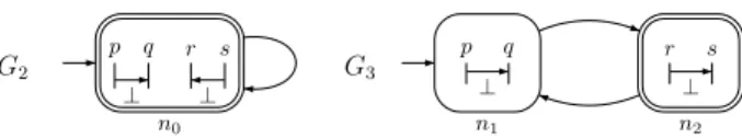
It immediately follows that if R is a set of represen-tatives for G, then L(G) = ∅ iff R = ∅. Now, many timed executions of a TC-MSC graph G are equiva-lent, in the sense that they are timed executions of the TC-MSC induced by the same final path of G. To check for emptiness of L(G), it suffices to con-sider emptiness of a set R of representatives for G, instead of L(G) itself. If R turns out to be regular and effective, then the emptiness problem for TC-MSC graphs can be decided. For example, consider G2 in Figure 2. The language L(G2) is not
regu-lar. However, the set {σ0, σ0σ1, σ0σ1σ2, . . .}, where
σi= (p!q, 4i)(q?p, 4i + 1)(s!r, 4i + 2)(r?s, 4i + 3) for
all i ∈ N, is a regular set of representatives for G2.
p q r s n0 ⊥ ⊥ G2 p q n1 ⊥ r s n2 ⊥ G3
Figure 2: Two TC-MSC graphs G2, G3. Specification G2 is
scenario-connected and G3 is not.
Thus, there are three elements in the technique of regular set of representatives: (1) choose a subset R of L(G), (2) show that R is a set of representatives for G and (3) prove that R is regular.
We fix TC-MSC graph G = (N, −→, nini, Nfin,
Λ, ∆), a path ρ = n0. . . nℓ of G, a timed execution
w = (a1, d1) . . . (ah, dh) of ρ, and e1. . . eh the
enu-meration of E associated with a1. . . ah. We start
by giving a first set of representatives.
Definition 3.2. Let K be an integer. We call w K-drift-bounded if for each 0 ≤ u ≤ ℓ, and i, j ∈ {1, . . . , h}, if ei, ejare in Λ(nu), then |di−dj| ≤ K.
Thus w is K-drift-bounded if the difference be-tween the first and last date associated with an event of any TC-MSC Λ(nu) is bounded by K.
In-terpreting the scenario in each node of a TC-MSC graph as one phase or transaction of a distributed protocol, it is realistic to believe that at least some (but not necessarily all) executions of an imple-mented system are K-drift-bounded.
Now, for a TC-MSC graph G and an integer K, we say that G is K-drift-bounded if for every con-sistent path ρ of G, there exists a K-drift-bounded timed execution in L(ρ). We emphasize that all timed executions of L(ρ) are not required to be K-drift-bounded. Observe that, G being K-drift bounded implies that the set LK(G) of
K-drift-bounded executions of G is a set of representatives of G. Unfortunately this set may not be regular. For example, G2in Figure 2 is K-drift-bounded for
K = 1, but LK(G2) is not regular for any K.
In-deed, for any K, the untimed projections of LK(G2)
and of Lt0(G
2), the timed language of G2where
ev-ery event occurs at date 0, are the same. As the un-timed projection of Lt0(G
2) is not regular, LK(G2)
is not (timed) regular.
For K′∈ N, w has at most K′ events per unit of
time if for any i, j ∈ {1, . . . , h}, dj− di≤ 1 implies
j − i < K′. A language L is strongly non-Zeno [5] if
there exists K′∈ N such that every execution of L
has at most K′events per unit of time. It turns out
that by imposing the following syntactical condi-tion, a TC-MSC graph has a strongly non-Zeno set of representatives (this is one consequence of Theo-rem 4.2 below). We say that a transition (n, n′) of
G is positively constrained if for every p, ∆p(n, n′)
is not [0, 0] (but can be [0, 1), [3, 3], [2, ∞) . . .). G is positively constrained if every transition of G is pos-itively constrained. This restriction does not imply that L(G) is itself strongly non-Zeno: consider the positively constrained TC-MSC graph G2of Figure
2 (where transitions without labels are implicitly labeled by ∆p= ⊥ for all p). L(G2) is not strongly
non-Zeno since unboundedly many events can oc-cur at date 0 (and hence within a unit of time). However, there exist timed executions where time elapses between positively constrained transitions.
We now present our regular set of representatives, namely the set LK,K′(G) of (K, K′)-well-behaved
timed executions, as well as the restriction needed on G for representativity.
Definition 3.3. For K, K′ ∈ N, we say that w is
(K, K′)-well-behaved if w is K-drift-bounded and
has at most K′ events per unit of time. Further a
TC-MSC graph is K-well-formed if it is K-drift-bounded and positively constrained.
4. Main results
We can now state our main results. The first two theorems below hold with one more technical re-striction imposed on TC-MSC graphs. However, the third theorem will establish decidability of the emptiness problem for TC-MSC graphs even with-out this technical restriction. A transition (n, n′)
of G is said to be scenario-connected if there exists a process p, s.t. both n and n′ have at least one p-event. G is scenario-connected if every transition of G is scenario-connected. For instance, in Figure 2, G2is scenario-connected while G3 is not.
Theorem 4.1. Let K, K′ ∈ N. If G is
scenario-connected, then LK,K′(G) is (timed) regular.
For representativity, we need G to be well-formed. Theorem 4.2. Let K ∈ N. If G is K-well-formed and scenario-connected, then LK,K′(G) is a set of
representatives of G, with K′ = (4(|P| + 1) + 2) ·
|P| · M , where M is the max number of events in a node of G.
Subsequently, in Proposition 5.3, we will prove that we can lift the the scenario-connected assumption, which along with Theorems 4.1 and 4.2 implies: Theorem 4.3. Given a K-well-formed TC-MSC graph G for some integer K, it is decidable to de-termine whether L(G) = ∅.
An immediate question is if, given a TC-MSC graph G and an integer K, one can decide whether G is K-well-formed. In fact, it turns out that this question is decidable. However, its proof involves vastly different techniques, and will be dealt with in a subsequent paper (see [16] for a draft). 5. Proofs of Main Results
Regularity: We prove Theorem 4.1 by construct-ing a timed automaton A which recognizes LK,K′(G). As in [15], A keeps track of nodes
that have not yet been fully executed, plus unex-ecuted events of these nodes. The property proved in Lemma 5.2 shows that it suffices to remember finitely many nodes and events (and thus finitely many clocks).
Throughout this section, let K, K′ ∈ N, and
ρ = n0. . . nz a (non necessarily final) path of a
scenario-connected TC-MSC graph G. Let w = (a1, d1) . . . (aℓ, dℓ) be a (K, K′)-well-behaved timed
execution of ρ. We denote by e1, . . . , eℓ the
enu-meration of events of Tρ associated with a
1, . . . , aℓ,
and d(ei) = di for all i. We also fix two constants
CK = (|P| + 1) · K and CK,K′= 2 · |P| · K′· CK.
Lemma 5.1. Let g be an event of node nj and g′ of
node nj′ of ρ, with j ≤ j′. Then d(g) ≤ d(g′) + CK.
Proof. Since G is scenario-connected, it follows that for each ntof ρ, there exists a process pt, an event
ft in nt and an event gt in nt+1 such that both
ft, gtare on process pt. Thus, there exists a
subse-quence of (ft, gt)j≤t≤j′ consisting of k ≤ |P| pairs
(fα(i), gα(i))1≤i≤k satisfying the following: (1) fα(1)
and g are in the same node, (2) fα(i+1) and gα(i)
are in the same node for each i < k, (3) g′ and
gα(k) are in the same node and (4) fα(i)and fα(i′)
are on different processes for all i 6= i′. Then,
we have fα(i) < gα(i) for each i ≤ k, as they are
on the same process. Hence d(fα(i)) ≤ d(gα(i)).
Also, |d(g) − d(fα(1))| ≤ K since g, fα(1) are in the
same node. Similarly, |d(fα(i+1)) − d(gα(i))| ≤ K
for each i ≤ k, and |d(gα(k)) − d(g′)| ≤ K. Thus,
d(g) ≤ d(g′) + (|P| + 1) · K (since k ≤ |P|).
The next lemma is the key for the regularity. Lemma 5.2. Let nxbe a node of ρ such that z−x ≥
CK,K′. For all e in nx and f in nz, d(e) < d(f ).
Proof. Recall that w has at most K′ events per
unit of time, and that each node of ρ contains at least one event. As z − x ≥ CK,K′ , there are m ≥
2K′× C
on the same process p, for some p ∈ P. Since w has at most K′ events per unit of time, it follows
that d(fm) > d(f1) + 2CK. Applying Lemma 5.1
to e, f1 and then again to fm, f , we obtain d(e) ≤
d(f1) + CK < d(fm) − 2CK+ CK≤ d(f ).
This lemma implies that taking aithe first event of
node nz appearing in w, every node nx with x ≤
z − CK,K′ has been fully executed before ai: for
every event ak of nx, we have k < i. We can now
sketch the construction of the timed automaton A: • States of A are sequences (n1, S1) · · · (nk, Sk),
such that k ≤ CK,K′, n1· · · nk is a (not
nec-essarily initial or final) path of G, for all i, Si is a suffix (for <ni) of Λ(ni) and S1 6= ∅.
(n0, Λ(n0)) is initial and (nf, ∅) is final.
Intu-itively, n1· · · nk are the last nodes of the path
seen during the execution, and Si is the set of
events not yet executed in ni. Since S1 6= ∅,
we can restrict to k ≤ CK,K′ using Lemma 5.2.
There is a clock associated with every event e inSi∈{1,...,k}Λ(ni), called the e-clock, and
ev-ery process p ∈ P, called the p-clock. • (n1, S1) · · · (nk, Sk) → (n′1, S1′) · · · (n′k′, S
′ k′) is
a transition of A if one of the following holds: action: k = k′, n′
j = nj for all j, there exists
i with Si = e · Si′ and Sj′ = Sj for all j 6= i.
Further, S1· · · Si−1 has no event on p(e). The
guard states that for all f in ni, the f -clock
is in δ(f, e), and if e is the first event of ni
on p, then the p-clock is in ∆p(ni−1, ni). The
transition resets the e-clock. Further, if e is the last event of nion p, then it resets the p-clock.
new node: k′ = k + 1 ≤ C K,K′ (n′ 1, S1′) · · · (n′k, Sk′) = (n1, S1) · · · (nk, Sk), nk→ n′k′ and Sk′′ = Λ(n′k′), deletion: k > 1, k′ = k − 1, S 1 = ∅ and (n′ 1, S1′) · · · (n′k′, Sk′′) = (n2, S2) · · · (nk, Sk).
It is easy but tedious to show L(A) = LK,K′(G).
Representativity: Now, we prove Theorem 4.2. Let ρ = n0. . . nz be a consistent path of G.
As G is bounded, there is a K-drift-bounded timed execution w = (a1, d1) . . . (aℓ, dℓ)
of Tρ. We construct another timed execution
w′ = (a
1, d′1) . . . (aℓ, d′ℓ) from w by suitably
mod-ifying the dates such that w′ is still an
execu-tion of Tρ and w′ is K-drift-bounded with at most
K′ = (4C
K+ 2) · |P| · M events per unit of time,
where M is the largest number of events in a node of G. The key idea in the construction of w′ is to
inductively postpone (when needed) the dates of all events of nx· · · nz. By postponing, we ensure that
there will exist some process p such that the differ-ence between the date of the last p-event of nx−1
and the date of the first p-event of nxis at least 1/2.
We use 1/2 since all intervals have integer bounds. We do not postpone if it is already the case.
As before, let e1. . . eℓ be an enumeration of
events in Tρ corresponding to a
1. . . aℓ, and let
us write d(e) (resp. d′(e)) for the date d i (resp
d′
i), when e = ei. To construct w′, we first
ini-tialize d′(e) = d(e) for each event e. Next,
con-sider node n1. Let Q be the set of processes
p that participate in both n0 and n1. As G is
scenario-connected, Q 6= ∅. For each p in Q, let lep(n0) denote the last p-event of n0 and fep(n1)
denote the first p-event of n1. If for some p ∈ Q,
d(fep(n1)) − d(lep(n0)) ≥ 1/2, then for each event
e in n1, do not modify d′(e) (it will not be
mod-ified later either). Otherwise, let θmax < 1/2 be
the maximum of d(fep(n1)) − d(lep(n0)) where p
ranges over Q. For each event e in n1. . . nz, set
d′(e) = d(e) + 1/2 − θ
max. We emphasize that when
considering node n1, the above procedure
post-pones dates of events in n1, and dates of events in
n2. . . nz, by the same amount. Since G is positively
constrained, the timed execution resulting from the above procedure is still in L(Tρ) and is still
K-drift-bounded. We inductively carry on the above procedure to consider each of the nodes n2, . . . , nz.
The timed execution w′ is obtained after
consider-ing all the nodes n0, . . . , nz. It follows that w′ is
K-drift-bounded and is in L(ρ).
It remains to show that w′has at most K′ events
per unit of time. It suffices to show that every pair of events e, f from two nodes nx, nz with z − x >
C = (4CK + 2) · |P| satisfies d′(f ) > d′(e) + 1.
Indeed, then, for each t, the set of events e with d(e) ∈ [t, t + 1) is included into the set of events of ny· · · ny+C for some y. There are at most K′ =
C × M such events, hence there are at most K′
events per unit of time.
If there are more than C = (4CK+ 2) · |P| nodes
between nxand nz, then there is some process p and
more than 4CK+2 pairs (fi, gi) of events in nx· · · nz
with fi the last p-event on some node nαi, gi is the
first event on node nα(i)+1, d′(gi) − d′(fi) ≥12, and
α is stricly increasing. This is by construction of w′. That is, d′(f
1) + 2CK + 1 < d′(gC+1). Now,
using Lemma 5.1 twice, for any event e of nx and
f of nz, we obtain d′(e) + 1 ≤ d′(f1) + CK+ 1 <
d′(g
C+1) − 2CK− 1 + CK+ 1 ≤ d′(f ).
Decidability: From Theorems 4.1 and 4.2, we readily conclude that, if G is scenario-connected, and K-well-formed, then one can decide whether L(G) is empty. It remains to lift the scenario-connected restriction to prove Theorem 4.3. Sup-pose G is not scenario-connected. Let NSC denote the set of transitions of G that are not scenario-connected. Proposition 5.3 states the crucial ob-servation that for any path ρ = n0· · · nℓ with
(ni, ni+1) in NSC for some i, the dates of events
in ni+1. . . nℓare not constrained in any way by the
dates of events in n0· · · ni. This fact was also used
in [9] along the same lines. Recall that in a transi-tion (n, n′), if some p ∈ P does not participate in either n or n′, then ∆
p(n, n′) = ⊥ = [0, ∞).
Proposition 5.3. Let ρ = n0· · · nℓ a path of G.
If (ni, ni+1) is in NSC then ρ is consistent iff both
n0· · · ni and ni+1· · · nℓ are consistent. If ρ is
con-sistent, (ni, ni+1), (nj, nj+1) are both in NSC and
ni= nj, then n0. . . ninj+1. . . nℓ is also consistent.
We now decompose G into a finite collection H of TC-MSC graphs, each of which is scenario-connected. We will decide the non-emptiness of L(G) by considering the non-emptiness of L(H) for every H in H, which is decidable as shown earlier. Let N1 be the subset of nodes n of G such that
(n′, n) ∈ NSC for some node n′ of G. Let N 2 be
the subset of nodes n′of G such that (n′, n) ∈ NSC
for some node n of G. For each n ∈ N1∪ {nini},
each n′∈ N
2∪Nfin, we build the scenario-connected
TC-MSC graph Hn,n′ from G as follows. The set
of nodes of Hn,n′ is the same as G. Hn,n′ has n as
initial node, and has one single final node n′. The transitions of Hn,n′consist of all scenario-connected
transitions of G. Let H be the collection of all such Hn,n′. For each Hn,n′ in H, we can decide whether
L(Hn,n′) is not empty since it is scenario-connected.
From Proposition 5.3(1), L(G) is not empty iff there exist a sequence Hn0,n1, Hn2,n3, . . ., Hn2ℓ,n2ℓ+1 in
H such that n0 = nini, n2ℓ+1 ∈ Nfin, and for each
i ≤ ℓ, L(Hn2i,n2i+1) is not empty and (n2i+1, n2i+2)
is in NSC . We can choose n0, n2. . . , n2ℓto be
dis-tinct according to Proposition 5.3(2). In particular, ℓ is at most the number of nodes of G.
6. Conclusion
In this paper, we have proved decidability of the language emptiness problem for a subclass of TC-MSC graphs. This problem was known to be un-decidable in general and un-decidable for regular TC-MSC graphs. The subclass considered in this paper
contains regular specifications and thus non-trivially extends the boundary of decidability. It is characterized in terms of bounds on the time a basic scenario takes, and disallows the constraint [0, 0] on transitions. We believe (see also [17]) that these two requirements do not impair implementability, and meet what designers have in mind when designing a TC-MSC graph: event execution takes time, and the specification is split in phases.
[1] S. Akshay, M. Mukund, and K. Narayan Kumar. Check-ing coverage for infinite collections of timed scenarios. In CONCUR 2007, LNCS 4703, pp. 181–196. Springer. [2] S. Akshay, P. Gastin, K. Narayan Kumar, and M. Mukund. Model checking time-constrained scenario-based specifications. In FSTTCS 2010, LNCS 4855, pp.
290–302. Springer.
[3] R. Alur and D. L. Dill. A theory of timed automata.
Theoretical Comp. Sci., 126(2):183–235, 1994.
[4] R. Alur and M. Yannakakis. Model checking of message sequence charts. In CONCUR 1999, LNCS 1664, pp.
114–129. Springer.
[5] C. Baier and T. Brihaye N. Bertrand, P. Bouyer. When are timed automata determinizable? In ICALP (2)
2009, LNCS 5556, pp. 43–54. Springer.
[6] P. Bouyer, S. Haddad, and P.-A. Reynier. Timed un-foldings for networks of timed automata. In ATVA
2006, LNCS 4218, pp. 292–306. Springer.
[7] F. Cassez, T. Chatain, and C. Jard. Symbolic unfold-ings for networks of timed automata. In ATVA 2006,
LNCS 4218, pp. 307–321. Springer.
[8] C. Dima and R. Lanotte. Distributed time-asynchronous automata. In ICTAC 2007, LNCS 4711,
185–200. Springer.
[9] P. Gastin, K. Narayan Kumar, and M. Mukund. Reach-ability and boundedness in time-constrained MSC graphs. In Perspectives in Concurrency – A
Fest-stichrift for P. S. Thiagarajan. Universities Press, 2009.
[10] B. Genest, D. Kuske, and A. Muscholl. A Kleene the-orem and model checking algorithms for existentially bounded communicating automata. Inf. and Comp., 204(6):920–956, 2006.
[11] J. G. Henriksen, M. Mukund, K. N. Kumar, M. So-honi, and P. S. Thiagarajan. A theory of regular MSC languages. Inf. and Comp., 202(1):1–38, 2005. [12] ITU-TS Recommendation Z.120: Message Sequence
Chart (MSC ’99), 1999.
[13] D. Lugiez, P. Niebert, and S. Zennou. A partial order semantics approach to the clock explosion problem of timed automata. TCS, 345(1):27–59, 2005.
[14] P. Madhusudan and B. Meenakshi. Beyond message sequence graphs. In FSTTCS 2001, LNCS 2245, pp.
256–267. Springer.
[15] A. Muscholl and D. Peled. Message sequence graphs and decision problems on mazurkiewicz traces. In MFCS
1999, LNCS 1672, pp. 81–91. Springer.
[16] S. Akshay, B. Genest, L. H´elou¨et, and S. Yang. Symbolically bounding the drift in time-constrained MSC graphs. Manuscript available at
http://www.crans.org/˜genest/AGHY12.pdf.
[17] S. Akshay, B. Genest, L. H´elou¨et, and S. Yang. Regular set of representatives for time-constrained MSC graphs. Technical Report RR-7823, HAL-INRIA, 2011.
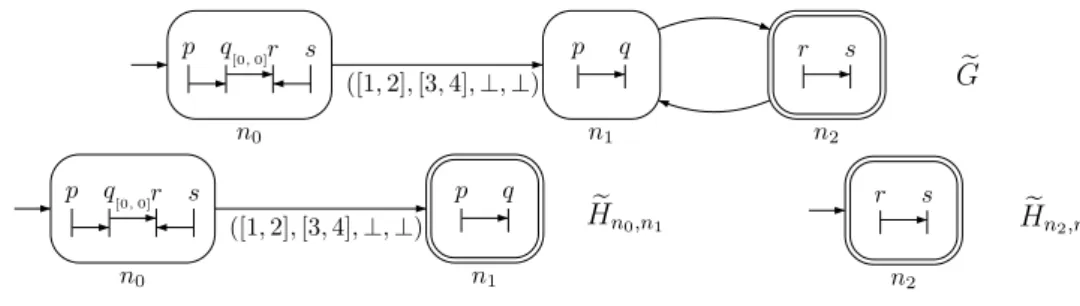
p q r s n0 [0,0] p q n1 ([1, 2], [3, 4], ⊥, ⊥) r s n2 e G p q r s n0 [0,0] p q n1 ([1, 2], [3, 4], ⊥, ⊥) Hen0,n1 r s n2 e H n2,n2
Figure 3: A TC-MSC graph eGwith unconstrained edges and its graph decomposition
Appendix
We give here the proof of Proposition 5.3. Proposition 5.3. Let ρ = n0· · · nℓ a path of G.
(1) If (ni, ni+1) is in NSC then ρ is consistent iff
both n0· · · ni and ni+1· · · nℓ are consistent. (2)If ρ
is consistent, (ni, ni+1), (nj, nj+1) are both in NSC
and ni = nj, then n0. . . ninj+1. . . nℓ is also
con-sistent.
We start by assuming wlog that a given TC-MSC graph G has a unique initial node n0and final node
nf(else we can add a dummy initial node and edges
from it to the old initial nodes and a dummy fi-nal node with edges from the old fifi-nal nodes to this one). Recall that (n1, n2) ∈ NSC if the
pro-cesses that participate in n1 and n2 are disjoint.
Observe that such edges are unconstrained by defi-nition, i.e., they can only have the timing constraint ⊥ = [0, ∞).
Proof. (1) One direction is straightforward. If ρ is consistent, then it means that we have a dated execution (w, d) corresponding to Tρ. Now,
pro-jecting (w, d) to events of n0· · · ni and ni+1· · · nℓ,
we respectively obtain a dated execution generated by Tn0···ni and Tni+1···nℓ. Thus, both Tn0···ni and
Tni+1···nℓ are consistent.
For the other direction, assume that both Tn0···ni
and Tni+1···nℓ are consistent, with timed
execu-tions (w1, d1) and (w2, d2). We can then obtain
the timed execution (w1w2, d) of Tρ by delaying
the timings sufficiently. More precisely, the timing d is obtained as d(e) = d1(e) for e ∈ n0· · · ni, and
d(e) = d2(e)+max for e ∈ ni+1· · · nℓ, where max is
the latest timing in d1. Indeed, such a delay in the
events is possible because we know that the edge (nini+1) is unconstrained and so a constant delay
in all the events will not affect any constraint in this execution Tρ. Thus (w
1w2, d) is a timed execution
of Tρ completing part(1) of the proof.
(2) Finally, assume that ρ is consistent, (ni, ni+1), (nj, nj+1) are both in NSC and ni =
nj. Consider a timed execution (w, d) of Tρ. We
first project it to events of n1· · · ni to obtain the
timed execution (w1, d1). We also project it to
events of nj+ 1 · · · nℓ to obtain the timed
execu-tions (w2, d2). Now, as above, the timed
execu-tion (w1w2, d′) with d′(e) = d1(e) for e ∈ n0· · · ni,
and d′(e) = d
2(e) + max for e ∈ ni+1· · · nℓ, where
max is the latest timing in d1 is an execution of
Tn0...ninj+1...nℓ, which is thus consistent.
With the above proof of Proposition 5.3, let us now demonstrate how the proof of Theorem 5.3 (de-cidability) works on a simple example. Consider the graph eG in Figure 3. Then (n1, n2) and (n2, n1)
are unconstrained edges and N1 = {n0, n2} and
N2 = {n1, n2} (the definitions of the sets N1 and
N2 are as in the last paragraph of Section 5). The
graph decomposition consists of eHn0,n1 and eHn2,n2
in the picture. Now observe that both eHn0,n1 and
e
Hn2,n2 are consistent (that it there exist accepting
paths) and (n1, n2) is unconstrained in eG. Thus
by Proposition 5.3 n0n1n2 is consistent and hence
L( eG) is non-empty, which indeed is also clear from the picture.