Descente d'échelle statistique du niveau de la mer pour les îles du Pacifique Sud-Ouest : une approche de régression linéaire multiple

(1)

THÈSE

En vue de l’obtention du

DOCTORAT DE L’UNIVERSITÉ DE TOULOUSE

Délivré par l'Université Toulouse 3 - Paul Sabatier

Présentée et soutenue par

Vandhna KUMAR

Le 18 octobre 2019

Descente d'échelle statistique du niveau de la mer pour les îles

du Paci-que Sud-Ouest - une approche de régression linéaire

multiple

Ecole doctorale : SDU2E - Sciences de l'Univers, de l'Environnement et de l'Espace

Spécialité : Océan, Atmosphère, Climat Unité de recherche :

LEGOS - Laboratoire d'Etudes en Géophysique et Océanographie Spatiale Thèse dirigée par

Alexandre GANACHAUD Jury

M. Christophe MAES, Rapporteur Mme Mélanie BECKER, Rapporteure

Mme Luciana FENOGLIO, Examinatrice Mme Déborah IDIER, Examinatrice M. Alexandre GANACHAUD, Directeur de thèse Mme Elisabeth HOLLAND, Co-directrice de thèse

Mme Mé

Mme Angélique MELET, M. Nicholas HALL,

Invitée

Établissement inscription, rang A

(2)

(3)

Statistical downscaling of island sea levels

in the southwest Pacific –

a multiple linear regression approach

by

Vandhna D. Kumar

A thesis submitted in fulfillment of the requirements for the degree of

Doctor of Philosophy

at

Université Toulouse III – Paul Sabatier in co-supervision with

Laboratoire d'Etudes en Géophysique et Océanographie (LEGOS), Toulouse Pacific Centre for Environment and Sustainable Development (PaCE-SD), Suva

(4)

(5)

i

Acknowledgements

I am grateful to many for their support and encouragement throughout this incredible thesis journey; I owe its sweet success and the many memories created along the way to them…

I would like to start with two of my pioneering mentors in the quest – Helene Jacot Des Combes, who was my supervisor from back during my Masters at PaCE-SD, and Dr. Awnesh Singh, who had freshly joined us as a postdoc back then. Their support kept me motivated in the direst days of my PhD opportunity hunt. Eventually, through them, I was introduced to Alexandre Ganachaud, who was looking for a student, and who later became my thesis director.

I extend heartfelt gratitude to my sponsors – the IPCC, IRD ARTS, and the USP Research office for jointly funding my study and for their commendable collaboration. I thank PaCE-SD, USP for being my home institution and for hosting me during my trips to Fiji. May our institutions continue to foster these exemplary partnerships as we strive towards resistance and capacity building against climate change in the Pacific.

Sincere thanks to my thesis director, Alex Ganachaud, a brilliant mentor and leader of our pedagogic committee. I continued to learn from your methodological approach and your proficiency, and am grateful for your continuous guidance. Big thanks to co-supervsior, Angélique Melet, whose efficiency and dedication to reviewing my numerous drafts remains unmatched. It was my good fortune to have your expertise in the team, and I thank you deeply for your commitment. I thank co-supervisor, Benoit Meyssignac, a true genius if I’ve met one. I remember days of perplexation and seemingly dead ends, only for them to be whisked away in seconds during discussions with Benoit.

Special thanks to co-supervisor Jerome Aucan, who contributed substantially despite being based far away from us, in Nouméa. Credit goes to Jerome for merging the two formerly separate tide gauge records for Nouméa and for recovering older records that had only existed in paper before. His contribution was not only towards the thesis, but to the larger sea level research community as well. I also thank Jerome for his assistance with my tide gauge data analysis.

Great contribution was also made by Billy Kessler, who provided the Rossby wave model used in this work. This was a key component of the analysis, and I thank Billy for his swift response and for sharing his expertise. It was a pleasure working with you, dear Billy.

I thank co-supervisor Awnesh Singh, our right-hand man for all our dealings with home institution, PaCE-SD, USP, back in Fiji. Thank-you for proficiently juggling the academic and administrative challenges this collaboration entailed.

Last but not least from our pedagogic committee, co-director Elisabeth Holland. Dear Elisabeth – I will be ever grateful for your support, understanding, and encouragement. In the ups and downs

(6)

ii

of my academic endeavors at PaCE-SD, I thank-you for being my rock. And thank-you for coming all the way from Fiji to attend my thesis defense.

The journey would not have been the same without my good friends and peers, of course!

Hearty thanks to my peers/mentors at LEGOS – Marine, Alice, Cori, Lise, Alejandro, Elvan, Hindu, Simon, Mariana, Fifi, Michel, and Cyril. I also thank Elodie, Malek, and Sylvain, and from PaCE-SD, Linda Yuen. And to my dearest friends Da and Sara, who I met at LEGOS – yours are the friendships I will forever cherish. Amidst the conversations and company of this lively circle, I always managed to find my strength whenever it was dwindling.

I am also very grateful to the LEGOS secretaries - Brigitte, Agathe, and especially Martine and Nadine for their constant assistance and support in all administrative matters. Special thanks for the warmth and welcome with which you always receive students.

Back at home, to my best friends Deepak and Shirleen – I am eternally grateful for your support and encouragement in my academic life and beyond. And to Nanna Emerly, with her kind and giving heart.

Thank-you for being part of my thesis journey…

(7)

iii The sea, at last, was as much his element as the land.

- Armstrong Sperry, The Boy Who Was Afraid (Call it Courage)

(8)

(9)

v

Auteur: Vandhna D. Kumar

Directeur de thèse: Alexandre Ganachaud

Titré de thèse: Descente d'échelle statistique du niveau de la mer pour les îles du Pacifique

Sud-Ouest - une approche de régression linéaire multiple

Discipline: Océanographie Physique

Lieu et date de soutenance: Observatoire Midi-Pyrénées, Toulouse, 8 Novembre, 2019 Laboratoire: LEGOS, UMR5566 CNRS/CNES/IRD/UPS, OMP, 14 Avenue Edouard Belin,

31400, Toulouse, France.

Résumé: L'élévation du niveau de la mer est une préoccupation croissante dans les îles du

Pacifique. Au cours de l'ère altimétrique (depuis 1993), les taux d'élévation du niveau de la mer sur le Pacific tropical ouest ont été parmi les plus élevés du monde, atteignant jusqu'à 3-4 fois la moyenne globale.

Alors que de plus en plus de communautés soumises aux risques associés à cette hausse du niveau de la mer se déplacent vers des terres plus élevées pour échapper à la montée des eaux, il est impératif de disposer de prédictions du niveau de la mer à l'échelle locale pour faciliter le processus d'adaptation et de planification. Ce processus n'est pas simple car le niveau de la mer varie d'une région à l'autre, notamment en fonction des redistributions de chaleur, sel et masses opérées aux échelles régionales par la circulation océanique, et des modes climatiques dominants (par exemple, ENSO, PDO/IPO). Même à l'échelle locale, d'importants changements du niveau de la mer relatif peuvent résulter de mouvements verticaux naturels ou anthropiques du sol terrestre.

Motivée par ces préoccupations, cette thèse se concentre sur l'utilisation d'une technique de descente d’échelle statistique basée sur des régressions linéaires multiples (MLR) pour modéliser les variations interannuelles-à-interdécennales du niveau de la mer pour trois sites côtiers localisés sur des îles du Pacifique Sud-Ouest - Suva et Lautoka à Fidji, et Nouméa en Nouvelle-Calédonie. Le modèle MLR est basé sur la connaissance que les variations du niveau de la mer à ces échelles de temps dans le Pacifique tropical sont principalement de nature thermostérique (c.-à-d. provenant des changements de densité de l’eau de mer induits par des changements de température de l'océan) et que ces variations thermostériques sont principalement générées par les variations de forçage de vent et les ondes de Rossby se propageant vers l’ouest qui en résultent.

Les expériences de MLR sont menées sur la période d'étude 1988-2014, l'accent étant mis sur la variabilité interannuelle à décennale et les tendances du niveau de la mer. Le niveau de la mer pour les trois sites côtiers insulaires est d'abord exprimé sous forme de somme des variations stériques et de masse. Dans un second temps, les modèles MLR développés se basent sur une approche plus orientée processus, en utilisant le rotationnel de tension de vent comme approximation de la composante thermostérique. Le niveau de la mer des îles est alors perçu comme une combinaison de composantes globale, régionales et locales, la seconde étant dominante. Le modèle MLR utilise le rotationnel de la tension de vent pour forcer un modèle

(10)

vi linéaire des ondes de Rossby. Les anomalies du niveau de la mer issues du modèle de Rossby sont utilisées comme régresseur régional dominant, alors que la composante halostérique locale (provenant des changements de densité de l’eau de mer induits par des changements de salinité de l'océan), la tension de vent locale et la température de surface de la mer locale sont utilisés comme régresseurs mineurs. Une régression par étapes est utilisée pour isoler les régresseurs statistiquement significatifs avant de calibrer le modèle MLR.

Le niveau de la mer prédit par la descente d’échelle statistique montre une forte concordance avec les observations, représentant en moyenne 80 % de la variance observée. Un test de stationnarité sur le modèle MLR montre qu'il peut être appliqué sur des périodes autres que celle utilisée pour la calibration, notamment pour les projections du niveau de la mer sur les décennies à venir. Dans l'ensemble, le niveau de la mer prédit par les modèles MLR donne un aperçu des principaux facteurs de la variabilité interannuelle-à-interdécennale du niveau de la mer sur les sites sélectionnés, montrant que si la dynamique locale et le signal global modulent le niveau de la mer dans une certaine mesure, la majeure partie de la variance est déterminée par des facteurs régionaux. Cela a des implications importantes pour les futures projections du niveau de la mer des îles - puisque les facteurs régionaux peuvent être simulés par des modèles climatiques, ils peuvent servir de lien entre les informations à l'échelle locale et les informations régionales à grande échelle fournies par les modèles climatiques à basse résolution. Les niveaux de la mer générés par la descente d’échelle statistique pourraient être utilisés comme source d’information pour élaborer des scénarios plus efficaces de planification de l'adaptation et de réduction des risques dans le Pacifique

Mots-clés: modèle statistique, régression linéaire multiple, niveau de la mer, îles, ouest

(11)

vii

Author: Vandhna D. Kumar

PhD director: Alexandre Ganachaud

Thesis title: Statistical downscaling of island sea levels in the southwest Pacific – a multiple

linear regression approach

Discipline: Physical Oceanography

Place and Date of defense: Observatory Midi-Pyrénées, Toulouse, 8 November, 2019 Laboratory: LEGOS, UMR5566 CNRS/CNES/IRD/UPS, OMP, 14 Avenue Edouard Belin,

31400, Toulouse, France.

Summary: Sea level rise is a growing concern in the islands of the western Pacific. Over the

altimetry era (1993-present), sea level rise rates in the western tropical Pacific were amongst the highest recorded across the world ocean, reaching up to 3-4 times the global mean. As more and more affected communities relocate to higher grounds to escape the rising seas, there is a compelling need for information on local scales to ease the adaptation and planning process. This is not a straightforward process as sea level varies regionally, driven by wind and ocean circulation patterns, and the prevailing climate modes (e.g. ENSO, PDO/IPO). On local scales, substantial sea level changes can result from natural or anthropogenic induced vertical ground motion.

Motivated by such concerns, this thesis focuses on developing a statistical downscaling technique, namely a multiple linear regression (MLR) model, to simulate island sea levels at selected sites in the southwest Pacific – Suva and Lautoka in Fiji, and Nouméa in New Caledonia. The model is based on the knowledge that sea level variations in the tropical Pacific are mainly thermosteric in nature (temperature-related changes in ocean water density) and that these thermosteric variations are dominated by wind-forced, westward propagating Rossby waves.

The MLR experiments are conducted over the 1988-2014 study period, with a focus on interannual-to-decadal sea level variability and trend. Island sea levels are first expressed a sum of steric and mass changes. Then, a more dynamical approach using wind stress curl as a proxy for the thermosteric component is undertaken to construct the MLR model. In the latter case, island sea levels are perceived as a composite of global, regional and local components, where the second is dominant. The MLR model takes wind stress curl as the dominant regional regressor (via a Rossby wave model), and the local halosteric component (salinity-related changes in ocean water density), local wind stress, and local sea surface temperature as minor regressors. A stepwise regression function is used to isolate statistically significant regressors before calibrating the MLR model.

The modeled sea level shows high agreement with observations, capturing 80% of the variance on average. Stationarity tests on the MLR model indicate that it can be applied skillfully to projections of future sea level. The statistical downscaling approach overall provides insights on key drivers of sea level variability at the selected sites, showing that while local dynamics and the global signal modulate sea level to a given extent, most of the variance is driven by

(12)

viii regional factors. This has important implications for future island sea level projections – since regional drivers can be simulated by climate models, it can serve as a link between high resolution, local scale information and low resolution climate models. The information generated can be used to guide more efficient adaptation planning and risk minimization practices in the Pacific.

Keywords: statistical downscaling, multiple linear regression, sea level, islands, western

(13)

ix

List of Figures

Chapter 2 – Literature review and background

Figure 2.1: Global sea level over the last 2,500 years ... 16

Figure 2.2: Altimetry-based GMSL time series over the 1993-2017 period.. ... 17

Figure 2.3: GMSL budget time series over the 2005-2012 period ... 19

Figure 2.4:Projections of global mean sea level rise over the 21st century relative to 1986– 2005 for RCP2.6 and RCP8.5. ... 24

Figure 2.4: Global, regional, and local sea levels in context: sea level trends across the globe from satellite altimetry for the period 1993-2012 (map) ... 27

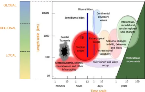
Figure 2.6: Schematic overview of local sea level processes. ... 28

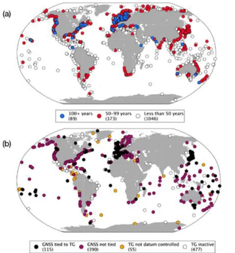
Figure 2.7: Tide gauge records available at the PSMSL database ... 30

Figure 2.8: Sketch showing basic observational quantities and techniques associated with sea level measurement ... 31

Figure 2.9: Sea level trends in the Pacific region over the 1993–2014 period from altimetry observations (GMSL trend included) ... 34

Figure 2.10: Schematic view of ocean and atmospheric conditions during the (a) neutral state, and anomalies during (b) El Niño and (c) La Niña. ... 36

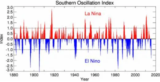
Figure 2.11: SOI time series from 1880 to 2013. Negative SOI values correspond to El Niño conditions (blue) and positive SOI values to La Niña conditions (red). ... 37

Figure 2.12: Spatial signature of IPO based SST anomalies. ... 38

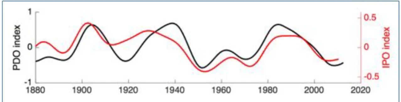
Figure 2.13: IPO and PDO index time series from 1880 to 2016. ... 39

Figure 2.14: The concept of spatial downscaling. ... 40

Figure 2.15: Map of the Fiji Islands, with study sites Suva and Lautoka marked. ... 43

Figure 2.16: Map of New Caledonia, with study site Nouméa marked. ... 43

Figure 2.17: Schematic representation of inter-linked processes and components of sea level change. ... 46

Chapter 3 - Methodology and datasets Figure 3.1: Illustration of the stepwise regression output (in Matlab) for the a given MLR experiment (undetrended, 1988-2014). . ... 51

Figure 3.2: Location of the Suva tide gauge (a, b) and GPS station (a, b, c). ... 55

Figure 3.3: Location of the Lautoka tide gauge (a, b, c) and GPS station (a, d). ... 55

Figure 3.4: Location of the Nouméa tide gauge (a, b) and GPS station (b), and the tide gauge inside the building. ... 55

(17)

xiii

Figure 3.5: 2-D correlation maps for selecting proxy boxes for the steric plus mass MLR

experiments for Suva (ORA-S4) over 2003-2014 (undetrended). ... 65

Figure 3.6: 2-D correlation maps for selecting proxy boxes for the steric plus mass MLR

experiments for Suva (tide gauge) over 2003-2014 (undetrended). ... 65

Figure 3.7: 2-D correlation maps for selecting proxy boxes for the main wind stress curl

dominated MLR experiments for Suva (ORA-S4) over 1988-2014 (undetrended). ... 68

Figure 3.8: 2-D correlation maps for selecting proxy boxes for the main wind stress curl

dominated MLR experiments for Suva (tide gauge) over 1988-2014 (undetrended). ... 68

Figure 3.9: 2-D correlation maps for selecting proxy boxes for MLR experiments using the

simplified approximation of the wind stress curl proxy for Suva (ORA-S4) over 1988-2014 (undetrended). ... 71

Chapter 4 - Evaluation of ORA-S4 steric fields - a site adapted approach

Figure 4.1: Island ORA-S4 steric sea-levels vs. the ORA-IP ensemble mean at

interannual-to-decadal timescales over 1993-2009 (including trend) ... 78

Figure 4.2: Island ORA-S4 thermosteric sea-levels vs. the ORA-IP ensemble mean at

interannual-to-decadal timescales over 1993-2009 (including trend). ... 79

Figure 4.3: Island ORA-S4 halosteric sea-levels vs. the ORA-IP ensemble mean at

interannual-to-decadal timescales over 1993-2009 (including trend). ... 80

Figure 4.4: 2-D correlation maps between island sea levels and the steric sea level fields for

selecting proxy boxes ... 83

Figure 4.5: Island sea-level time series (ORA-S4) vs. ORA-S4 steric component in the upper

(700 m) and deeper oceans (700 m – bottom) at interannual-to-decadal timescales over 1988-2014 (including trend) ... 84

Figure 4.6: Island sea-level time series (ORA-S4) vs. ORA-S4 thermosteric component in the

upper (700 m) and deeper oceans (700 m – bottom) at interannual-to-decadal timescales over 1988-2014 (including trend) ... 85

Figure 4.7: Island sea-level time series (ORA-S4) vs. ORA-S4 halosteric component in the

upper (700 m) and deeper oceans (700 m – bottom) at interannual-to-decadal timescales over 1988-2014 (including trend) ... 85

Figure 4.8: Time series of island thermosteric and halosteric sea-levels in the upper 700 m at

interannual-to-decadal timescales over 1988-2014 (including trend) ... 87

Chapter 5 - Results

Figure 5.1: Interannual sea-level time series at Suva (top panel), Lautoka (middle panel) and

Nouméa (bottom panel) over the 1988-2014 period... 92

Figure 5.2: Regressor and predictand time series at interannual-to-decadal timescales for the

(18)

xiv

Figure 5.3: Regressor and predictand time series at interannual-to-decadal timescales for the

steric plus mass MLR experiments (undetrended) over 2003-2014 ... 96

Figure 5.4: MLR modeled and predictand sea level time series at interannual-to-decadal

timescales for the steric plus mass MLR experiments (detrended) over 2003-2014 ... 100

timescales for the steric plus mass MLR experiments (undetrended) over 2003-2014 ... 101

timescales for the main wind stress curl (Rossby wave model) dominated MLR experiments (detrended) over 1988-2014 ... 104

timescales for the main wind stress curl (Rossby wave model) dominated MLR experiments (undetrended) over 1988-2014 ... 105

Figure 5.8: Site-based thermosteric sea level and wind stress curl (Rossby wave model) proxy

based thermosteric regressor time series at interannual-to-decadal timescales for the main MLR experiments (detrended) over 1988-2014 ... 108

Figure 5.9: Site-based thermosteric sea level and wind stress curl (Rossby wave model) proxy

based thermosteric regressor time series at interannual-to-decadal timescales for the main MLR experiments (undetrended) over 1988-2014 ... 109

Figure 5.10: MLR modeled and predictand sea level time series (ORA-S4 only) at

interannual-to-decadal timescales for the simplified approximation method MLR experiments (detrended) over 1988-2014. ... 113

Figure 5.11: MLR modeled and predictand sea level time series (ORA-S4 only) at

interannual-to-decadal timescales for the simplified approximation method MLR experiments (undetrended) over 1988-2014. ... 114

Figure 5.12: Site-based thermosteric sea level and wind stress curl proxy based thermosteric

regressor time series at interannual-to-decadal timescales for the simplified approximation method MLR experiments (detrended) over 1988-2014 ... 115

Figure 5.13: Site-based thermosteric sea level and wind stress curl proxy based thermosteric

regressor time series at interannual-to-decadal timescales for the simplified approximation method MLR experiments (undetrended) over 1988-2014 ... 116

Figure 5.14: Stationarity test for the main wind stress curl (Rossby wave model) dominated

MLR experiments (detrended) over 1988-2014 (interannual-to-decadal timescales) ... 118

Figure 5.15: Stationarity test for the main wind stress curl (Rossby wave model) dominated

MLR experiments (undetrended) over 1988-2014 (interannual-to-decadal timescales) ... 119

Figure 5.16: Stationarity test for the simplified approximation method MLR experiments

(detrended) over 1988-2014 (interannual-to-decadal timescales)... 120

Figure 5.17: Stationarity test for the simplified approximation method MLR experiments

(19)

xv

Chapter 6 - Discussion

Figure 6.1: Island sea level for the study sites (ORA-S4) correlated with the basin-wide

thermosteric sea level (a, c, e) and the Rossby wave modeled thermosteric change (b, d, f) at interannual-to-decadal time scales over 1988-2014 (undetrended). ... 135

Figure .2: Time series of the Niño 3.4, IPO indices versus the dominant wind stress curl

(20)

xvi

List of Tables

Chapter 2 – Literature review and background

Table 2.1: Global mean sea level budget (mm/yr) over different intervals within the 20th_and

early 21st_{century from observations and model simulations. ... 18}

Chapter 3 – Methodology and datasets

Table 3.1: Tide gauge station data for Suva, Lautoka, and Nouméa, with longitude/latitude

coordinates, data duration, and percentage of missing data. ... 54

Table 3.2: Proxy box bounds (longitude/latitude) for the thermosteric and halosteric

regressors for the steric plus mass MLR experiments over 2003-2014. ... 66

Table 3.3: Proxy box bounds (longitude/latitude) for all regressors (Rossby wave SLA,

halosteric SLA, zonal and meridional wind stress, and SST) for the wind stress curl dominated MLR experiments over 1988-2014. ... 69

Table 3.4: Proxy box bounds (longitude/latitude) for all regressors (wind stress curl, halosteric

SLA, zonal and meridional wind stress, and SST) for the MLR experiments using the simplified approximation of the wind stress curl proxy over 1988-2014. ... 72

Chapter 4 – Evaluation of ORA-S4 steric fields – a site adapted approach

Table 4.1: Correlation coefficient (r) between island steric, thermosteric, and halosteric

sea-levels from ORA-S4 and ORA-IP reanalysis ensemble mean, and ratio of standard deviations

of ORA-S4 time series to the ensemble mean (σORA-S4/σens.) at interannual-to-decadal

timescales over 1993-2009 (including trend) ... 81

Table 4.2: Trends of island steric, thermosteric, and halosteric sea-levels from ORA-S4 and

ORA-IP reanalysis ensemble mean over 1993-2009. ... 82

Table 4.3: Correlation coefficient (r) between island sea-levels (ORA-S4) and ORA-S4 steric,

thermosteric, and halosteric components in the upper (700 m) and deeper oceans (700 m –

bottom), and percentage variance (R2_{) explained by each at interannual-to-decadal timescales}

over 1988-2014 (including trend) ... 86

Table 4.4: Correlation coefficient (r) between the thermosteric and halosteric sea-levels in

the upper 700 m at interannual-to-decadal timescales over 1988-2014 (including trend) ………...……….…...… 87

Chapter 5 - Results

Table 5.1: Sea-level trends (mm/yr) from tide gauge, ORA-S4 and altimetry at Suva,

Lautoka and Nouméa over the 1988-2014 and 1993-2014 periods. ... 93

Table 5.2: Correlation coefficient (r) between tide gauge, ORA-S4, and altimetry sea-level

(21)

xvii

Table 5.3: Correlation coefficient (r) between the predictand and individual regressors

(thermosteric SLA, halosteric SLA, and mass change), and percentage variance (R2_{) explained}

by each for the steric plus mass MLR experiments over 2003-2014. ... 97

Table 5.4: Equations (regression coefficients) of the steric plus mass MLR models over

2003-2014 ... 98

Table 5.5: Correlation coefficient (r) between the predictand (ORA-S4, tide gauges) and

MLR modeled sea-levels, and percentage variance (R2_{) explained by the MLR model for all}

experiments (simplified approximation method MLR experiments conducted with ORA-S4 sea-levels only). ... 102

Table 5.6: Predictand (ORA-S4, tide gauges) and MLR modeled sea-level trends for all

experiments with undetrended data. ... 106

Table 5.7: Equations (regression coefficients) of the wind stress curl (Rossby wave model)

dominated MLR models over 1988-2014... 107

Table 5.8: Correlation coefficient (r) between the thermosteric sea-level and wind stress curl

regressor (Rossby wave model derived thermosteric approximated proxy), and percentage

variance (R2_{) explained by the thermosteric proxy for the wind stress curl dominated and the}

simplified approximation method MLR experiments (conducted with ORA-S4 sea-levels only)... 110

Table 5.9: Equations (regression coefficients) of the simplified approximation method MLR

models over 1988-2014. ... 114

Table 5.10: Stationarity test statistics - correlation coefficient (r) between the predictand

(ORA-S4, tide gauges) and MLR modeled sea-levels, and percentage variance (R2_{) explained}

by the MLR model for the wind stress curl dominated (Rossby wae model) MLR experiments over 1988-2014. ... 122

Table 5.11: Stationarity test statistics - correlation coefficient (r) between the predictand

(ORA-S4, tide gauges) and MLR modeled sea-levels, and percentage variance (R2_{) explained}

by the MLR model for experiments using the simplified approximation of the wind stress curl proxy over 1988-2014. ... 123

Table 5.12: Stationarity test MLR trends for all experiments with undetrended datasets over

1988-2014 ... 124

Chapter 6 – Discussion

Table 6.1: Correlation coefficient (r) between the Niño 3.4, IPO indices and the (1) dominant

wind stress curl regressor, (2) island sea level for the main (Rossby wave model) MLR experiments over 1988-2014 ... 142

(22)

(23)

xix

List of Abbreviations

AMMA – African Monsoon Multidisciplinary Analysis APB – Autonomous Pinniped Bathythermograph AR5 – Assessment Report 5

CCA – Canonical Correlation Analysis CTD – Conductivity, Temperature, Depth

CLARIS – Climate Change Assessment and Impact Studies CMEMS – Copernicus Marine Environment Monitoring Service CMIP5 – Coupled Model Intercomparison Project phase 5

CSIRO – Commonwealth Scientific and Industrial Research Organization CORDEX – Coordinated Regional Climate Downscaling Experiment CSR – Center for Space Research

DUACS – Data Unification and Altimeter Combination System ECMWF – European Center for Medium-Range Weather Forecasts ENSO – El Niño Southern Oscillation

EOF – Empirical Orthogonal Analysis ERA – ECMWF Re-Analysis

GCM – General Circulation Model GFZ – GeoForschungsZentrum GMSL – Global Mean Sea Level

GNSS – Global Navigation Satellite Systems GPS – Global Positioning System

GRACE – Gravity Recovery and Climate Experiment GRGS – Groupe de Recherche de Geodesie Spatiale IFS – Integrated Forecasting System

IPCC – Intergovernmental Panel on Climate Change IPO – Interdecadal Pacific Oscillation

IRD – Institut de Recherche pour le Développement ITCZ – Inter Tropical Convergence Zone

JPL – Jet Propulsion Laboratory

LEGOS – Laboratoire d’Études en Géophysique et Océanographie Spatiales MEI – Multivariate ENSO Index

MEDRYS – MEDiterranean sea ReanalYsiS MLR – Multiple Linear Regression

(24)

xx

NEMO – Nucleus for European Modeling of the Ocean NEMOVAR – NEMO variational data assimilation

OCHA – United Nations Office for the Coordination of Humanitarian Affairs OGCM – Ocean General Circulation Model

OMP – Observatoire Midi-Pyrénées

ORA-IP – Ocean Re-Analysis Intercomparison Project ORA-S3 – Ocean Re-Analysis System 3

ORA-S4 – Ocean Re-Analysis System 4

PaCE-SD – Pacific Centre for Environment and Sustainable Development PDO – Pacific Decadal Oscillation

PRUDENCE – Prediction of Regional scenarios and Uncertainties for Defining EuropeaN

Climate change risks and Effects

PIRATA – Prediction and Research Moored Array in the Tropical Atlantic PSMSL – Permanent Service for Mean Sea Level

RAMA – Research Moored Array for African-Asian-Australian Monsoon Analysis RCP – Representative Concentration Pathway

REFMAR – Réseaux de référence des observations marégraphiques RLR – Relative Local Reference

RMSE – Root Mean Square Error SLA – Sea Level Anomaly

SLP – Sea Level Pressure

SOI – Southern Oscillation Index

SONEL – Système d'Observation du Niveau des Eaux Littorales SPCZ – South Pacific Convergence Zone

SPM – Summary for Policy Makers

SSALTO – Segment Sol Multimission Altimetry and Orbitography SSH – Sea Surface Height

SST – Sea Surface Temperature

STARDEX – STAtistical and Regional dynamical Downscaling of EXtremes for European

regions

SVD – Singular Vector Decomposition TAO – Tropical Atmosphere Ocean ToE – Time of Emergence

TNI – Trans-Niño Index

TOPEX-Poseidon – Topography Experiment - Positioning, Ocean, Solid Earth, Ice Dynamics,

Orbital Navigator

(25)

xxi

TUG – Graz University of Technology WMO – World Meteorological Organization XBT – Expendable BathyThermograph

(26)

(27)

1

Introduction générale (en français)

Motivation

L’Océan Pacifique est le plus vaste océan du monde. Couvrant environ un vaste tiers de la surface de la Terre, l'océan Pacifique abrite de nombreux petits États insulaires en développement (PEID). L'océan est profondément enraciné dans les identités culturelles du Pacifique et joue un rôle important pour les moyens d’existence et les économies insulaires, sous-tendant des secteurs comme la pêche, le tourisme, la sécurité alimentaire, les transports et les loisirs. En englobant la plus grande zone océanique tropicale de la planète, le Pacifique est aussi le centre d'action de phénomènes climatiques majeurs comme El Niño Southern Oscillation et la Pacific Decadal Oscillation / Interdecadal Pacific Oscillation (PDO/IPO), et représente donc une zone d’intérêt pour la recherche sur le climat et l’océan. Au cours des dernières décennies, le Pacifique a enregistré les taux les plus élevés d'élévation du niveau de la mer dans le monde, ce qui a suscité un vif intérêt de la part de la communauté mondiale des chercheurs sur le climat et le niveau de la mer (e.g. Becker et al. 2012 ; Meyssignac et al. 2012 ; Han et al. 2014 ; Palanisamy et al. 2015a ; Marcos et al. 2017). L'élévation du niveau de la mer est une conséquence directe du changement climatique en cours. Les tendances récentes du niveau de la mer présentent un aléa pour les zones côtières. Combiné à l’exposition des populations insulaires vivant en zone côtière et à la vulnérabilité de ces îles face au changement climatique et à la hausse du niveau de la mer (facteurs typiques tels que l'isolement géographique, le stress économique, les contraintes financières et le manque d'expertise humaine et technique), l’aléa associé à la hausse du niveau de la mer devient un risque majeur associé au changement climatique pour ces états insulaires du Pacifique (e.g. Barnett et Campbell 2010 ; Wong et al, 2014 ; Garschagen et al, 2016). Contrairement aux menaces à long-terme et/ou sporadiques liées au climat, l'élévation du niveau de la mer ne représente plus un risque pour le futur lointain ou un risque peu fréquent mais une réalité déjà présente dans de nombreuses zones côtières (Hallegatte et al. 2013 ; Wong et al. 2014 ; Neumann et al. 2015). Si les atolls coralliens de faible altitude sont certainement plus menacés que les îles volcaniques présentant des altitudes plus importantes, même ces dernières ont vu des communautés forcées de se déplacer en raison de l'intrusion d'eau salée dans les eaux de surface (sur terre) et les nappes phréatiques, de niveaux de la mer élévés pendant les périodes de vives-eaux des marées de périgée et des crues subites lors des événements extrêmes (Nurse et al. 2014 ; OCHA-ONU 2014 ; McNamara & Jacot Des Combes 2015 ; Albert et al. 2016).

A mesure que le réchauffement planétaire se poursuit, l'expansion thermique de l'eau de mer, la fonte des glaciers et la perte de masse des calottes glaciaires entraîneront une augmentation de l'élévation du niveau moyen de la mer (Jevrejeva et al. 2010 ; Church et al. 2011 ; Church et al. 2013) qui aggravera les impacts côtiers associés au niveau de la mer (inondations, intrusion saline, …). Compte tenu des trajectoires actuellement suivies pour les émissions de gaz à effet de serre, du réchauffement planétaire asssocié (Boyd et al. 2015 ; Höhne et al. 2017 ; Millar et al. 2017) et de la

(28)

2

mémoire longue des océans associées aux échelles de temps longues de la circulation profondes (Rhein et al. 2013), l'option la plus viable pour les îles menacées est une planification efficace des mesures d'adaptation et de réduction des risques. Pour que ces stratégies soient efficaces, il est essentiel de disposer d'informations solides à l'échelle locale.

De nos jours, les modèles numériques de climat sont les outils privilégiés pour comprendre le système climatique et sa prévisibilité à différentes échelles de temps et sous différentes perturbations. L'information provenant des modèles de climat sert à orienter les études de détection et d'attribution pour évaluer dans quelle mesure les changements observés sur la période instrumentale sont à attribuer au changement climatique (forçage anthropogénique) ou à la variabilité interne du système climatique. Les modèles de climat permettent également de produire des projections des conditions climatiques et océaniques sur les décennies et siècle(s) à venir. Ces informations sont essentielles au processus décisionnel des parties prenantes dans divers domaines tels que l'agriculture, la pêche, les infrastructures, l'urbanisme, la sécurité alimentaire et en eau, l'énergie, les transports, les assurances, l'adaptation, la prévention des risques, etc. Cependant, les incertitudes associées aux variables simulées par les modèles de climat deviennent plus importantes quand on s’intéresse à des échelles spatiales de plus en plus fine. Ceci est en partie du aux résolutions spatiales généralement grossières (~100 km) de ces modèles. Avec les résolutions utilisées dans les composantes océaniques des modèles de climat actuels, les petites îles ne sont pas résolues et sont perçues comme faisant partie de l'océan.

Cette thèse est motivée par le besoin urgent de disposer d'informations fiables sur le niveau de la mer à l'échelle locale, qui peuvent aider pour élaborer des mesures efficaces d'adaptation et de réduction des risques.

Le processus de génération d'information à haute résolution ou à l'échelle locale à partir de d’information à grande échelle est connu sous le nom de descente d’échelle (downscaling en anglais). Dans cette thèse, une technique de descente d'échelle statistique est utilisée pour reconstituer le niveau de la mer pour certains sites côtiers des îles du Pacifique Sud-Ouest - Suva et Lautoka dans les îles Fidji, et Nouméa en Nouvelle-Calédonie. Basée sur les connaissances existantes sur les processus responsables des variations régionales et locales du niveau de la mer dans le Pacifique tropical, l'approche utilise une combinaison de variables océaniques/atmosphériques comme prédicteurs pour formuler un modèle de régression linéaire multiple (multiple linear regression –MLR- en anglais) du niveau de la mer insulaire. Le niveau de la mer local ainsi modélisé à partir de variables à grande échelle présente une grande similitude (corrélation, variance expliquée) avec le niveau de la mer observé et peut être utilisé pour générer des projections des changements futurs du niveau de la mer à l'échelle locale et raffiner à l’échelles locale les modèles climatiques à grande échelle. L'approche peut également être adaptée à d'autres sites, en ajustant les combinaisons de variables fournissant l’information de grande échelle au besoin.

(29)

3

Les informations à l’échelle locale peuvent être utilisées par les parties prenantes et les décideurs pour affiner la planification de l'adaptation et de la réduction des risques. De cette façon, les résultats scientifiques sur la probabilité de changements futurs peuvent être appliqués jusqu'aux politiques et canaux et de mise en œuvre, devenant ainsi une partie du renforcement de la résilience dans le Pacifique.

Périmètre de l'étude

Cette thèse vise à construire un modèle statistique de descente d'échelle pour les variations interannuelles à inter-décennales du niveau de la mer pour trois sites côtiers situés sur des îles du Pacifique sud-ouest. Dans l'approche de descente d'échelle utilisée dans cette thèse, le niveau de la mer à un site donné (local) est fonction de régresseurs potentiels représentant des facteurs régionaux (à grande échelle) et locaux (à petite échelle) superposés à la moyenne globale (von Storch et al. 2000 ; Benestad et al. 2007). Le concept est appliqué aux sites d'étude sélectionnés à l'aide d'une régression linéaire multiple (MLR), un ensemble de variables océaniques et atmosphériques servant de régresseurs. Les variables explicatives permettent de représenter le niveau régional de la mer, qui s'avère dominant pour les trois sites étudiés ici, et les signatures locales. La moyenne globale est retirée du prédictand (niveau de la mer observé servant à calibrer le modèle MLR).

Dans la région du Pacifique, comme dans la plupart des régions du globe, les variations du niveau de la mer sont largement de nature stérique (i.e. liés à des changements de volume de l’océan induits par des changements de densité de l’eau de mer) avec une prédominance de la composante thermostérique (liées aux changements de densité induit par les changements de température). Aux échelles de temps interannuelles à décennales, les variations du niveau de la mer thermostérique sont en majeur partie générées par les variations de la tension du vent sur le bassin tropical (p. ex. Carton et al. 2005 ; Köhl et al. 2007 ; McGregor et al. 2012 ; Nidheesh et al. 2013 ; Timmermann et al. 2010). Les anomalies de rotationnel de tension de vent contrôlent la profondeur de la thermocline et le niveau de la mer stérique qui, en bonne approximation pour cette région, en est le miroir, en modulant le transport d’Ekman près de la surface, le pompage Ekman et la propagation vers l'ouest des ondes de Rossby. En tant que tel, les changements de la tension du vent représentent un facteur déterminant des tendances et des variations du niveau de la mer dans la région.

Dans le Pacifique Ouest, la propagation des ondes de Rossby explique la majeure partie de la variabilité du niveau de la mer (Fu et Qiu 2002 ; Qiu et Chen 2006 ; Lu et al. 2013) et un modèle linéaire en eau peu profonde à gravité réduite (modèle des ondes de Rossby) est utilisé pour modéliser la réponse du niveau de la mer thermostérique aux variations du forçage en vent. Le niveau de la mer fournit par le modèle d’ondes de Rossby s'avère être le principal régresseur dans le modèle de descente d’échelle MLR.

(30)

4

Une fonction de régression par étapes est d'abord utilisée pour isoler les régresseurs statistiquement significatifs, qui sont ensuite utilisés pour calibrer le modèle MLR. Les autres variables explicatives représentent les effets locaux : niveau de la mer halostérique, tension de vent et température de surface de l’océan pour, représenter respectivement, les flux d'eau douce, les surcotes liées au vent et les flux de chaleur de surface.

Comme la motivation sous-jacente à l'élaboration du modèle MLR est une application aux projections futures du niveau de la mer, la capacité du modèle à générer une information pertinente sur des périodes autres que celle sur laquelle il a été calibré est évaluée par un test de stationnarité. La performance du modèle sur des périodes autres que celles sur lesquelles il a été calibré est alors évaluée à la lumière du modèle MLR utilisé à plein potentiel.

L'analyse MLR est effectuée à la fois en utilisant des séries temporelles du niveau de la mer issues de l’estimation de l'état de l'océan (réanalyse ORA-S4) et de marégraphes in situ pour calibrer le modèle. Cependant, du fait que la réanalyse du niveau de la mer fait déjà partie de la méthodologie, la correction du mouvement vertical du sol (affaissement, soulèvement) affectant les enregistrements de marégraphes n'entre pas dans le cadre de cette thèse; les résultats sont plutôt pris en compte sur la base d'un tel mouvement lorsque des preuves sont disponibles (littérature, enregistrements, altimétrie).

L'étendue de la thèse va jusqu'au processus de calibration et du test de stationnarité du modèle MLR. Bien que l'application du modèle développé aux données CMIP5 a été plus que souhaitée, elle n'a pas été couverte en raison des contraintes de temps. Cependant, il est fortement prévu que les expériences MLR-CMIP5 soient poursuivies dans une étude de suivi.

Objectifs

Les objectifs de cette thèse sont les suivants :

i. Élaborer une régression linéaire multiple pour les variations interannelles à interdécennales du niveau de la mer pour trois sites insulaires en utilisant des variables océaniques/atmosphériques régionales et locales.

ii. Permettre une meilleure compréhension de l'importance relative des processus physiques pour les changements locaux du niveau de la mer sur les sites d'étude.

iii. Évaluer la performance globale du modèle MLR et identifier les sources d'erreur et la variance inexpliquée du modèle utilisé pour le niveau de la mer.

iv. Évaluer la stationnarité du modèle MLR développé par rapport aux projections futures du niveau de la mer.

(31)

5

Plan de thèse

Après cette brève introduction, où la motivation, la portée et les objectifs de la thèse sont présentés, un aperçu plus complet des variations du niveau de la mer, de ses causes physiques et de la réduction d'échelle est fourni au Chapitre 2 - Revue de la littérature et contexte. Le Chapitre 2 décrit le contexte plus large de cette thèse, couvrant un éventail de sujets tels que le niveau de la mer mondial et régional, les tendances du niveau de la mer du Pacifique, les modes climatiques régionaux tels que ENSO et IPO / PDO, et les méthodes de réduction d'échelle, et introduit les sites d'étude. Les ensembles de données utilisés et les expériences menées sont ensuite décrits au Chapitre 3. Au Chapitre 4, la méthode de sélection du produit de réanalyse, ORA-S4, qui est la source de certains des principaux ensembles de données utilisés dans la thèse, est pré-évaluée pour la région d'étude.

Les résultats sont fournis dans le Chapitre 5, reliant et développant sur l'article revu et publié durant la période de travail de cette thèse.

La discussion du Chapitre 6, en plus d'étendre les résultats de l'étude, décrit le modèle MLR développé dans le contexte d'autres initiatives de réduction d'échelle du niveau de la mer du monde entier et discute des préoccupations pratiques pour de futures applications.

Enfin, la conclusion et les recommandations sont présentées au Chapitre 7.

Des documents supplémentaires sont fournis en annexe. L'article revu et publié durant cette thèse est inclus dans l'annexe 1, et les contenus des affiches présentées lors des conférences et réunions internationales sont ajoutés dans l'annexe 2.

(32)

(33)

7

Chapter 1 Introduction

1.1 Motivation ... 9 1.2 Scope of the thesis ... 10 1.3 Objectives ... 11 1.4 Thesis outline ... 12

(34)

(35)

9

1. Introduction

1.1 Motivation

The Pacific is the world’s largest ocean. Covering roughly a vast one third of the Earth’s surface area, the Pacific Ocean is home to numerous small island developing states (SIDS). The ocean is rooted deeply into Pacific cultural identities as well as island livelihoods and economies, underpinning sectors such as fisheries, tourism, food security, transportation and recreation. Encompassing the planet’s largest tropical ocean zone, the Pacific is also the origin and center of action of major climatic phenomenon like the El Niño Southern Oscillation (ENSO) and the Pacific Decadal Oscillation (PDO)/ Interdecadal Pacific Oscillation (IPO), and thus a hotspot for climate and ocean research. Over recent decades, the Pacific has recorded the highest rates of sea level rise across the globe, spurring keen interest from the climate and sea level research community worldwide (e.g. Becker et al. 2012; Meyssignac et al. 2012; Han et al. 2014; Palanisamy et al. 2015a; Marcos et al. 2017).

Sea level rise is a critical consequence of global warming and recent climate change. Recent sea level trends, combined with typical factors such as geographical isolation, economic stress, financial constraints, and lack of both human and technical expertise make the Pacific islands amongst the most vulnerable to ongoing climate and sea level changes (e.g. Barnett & Campbell 2010; Nicholls and Cazenave 2010; Wong et al., 2014; Garschagen et al. 2016;). Unlike long-term and/or sporadic climate-related threats, rising sea levels are no longer a distant or infrequent hazard but present reality in many coastal zones (Hallegatte et al. 2013; Wong et al. 2014; Neumann et al. 2015). While low-lying coral atolls are certainly more endangered than high rise volcanic islands, even the latter have had communities forced to relocate due to saltwater intrusion, perigean spring tides, and flash floods during extreme events (Hallegatte et al. 2013; Nurse et al. 2014; OCHA—United Nations 2014; McNamara & Jacot Des Combes 2015; Albert et al. 2016; Hinkel et al. 2019).

As global warming continues, thermal expansion of seawater, and melt of glaciers and ice sheets will lead to committed global mean sea level rise (e.g. Church et al. 2013; Levermann et al. 2013; Golledge et al. 2015; Mengel et al. 2018) exacerbating coastal impacts. Based on ongoing emission trajectories (Boyd et al. 2015; Höhne et al. 2017; Millar et al. 2017) and the slow thermal feedback of the ocean (Rhein et al. 2013), the more viable option on threatened islands is efficient adaptation. For such strategies to be effective, local scale information is essential (e.g. refined estimates of projected sea level changes, unambiguous probabilistic projections, best and worst-case scenarios of sea-level rise, etc. (e.g. Hinkel et al. 2019)).

In the present day, climate models serve as central tools for understanding the climate system and its predictability on various timescales and under different perturbations. Information from climate models is used to guide detection and attribution studies in the context of recent climate change and to generate projections of climate/ocean conditions on decadal to centennial timescales. This information is key in the decision-making process for policymakers across various domains such as

(36)

10

agriculture, fisheries, infrastructure, urban planning, food/water security, energy, transportation, insurance, adaptation, risk prevention, etc. Yet, while climate models are reliable for large-scale simulations, their skill is greatly reduced at small scales due to typically coarse spatial resolutions (~100 km for the ocean component). At this resolution, smaller islands are not well represented in the model, remaining unresolved and being perceived largely as part of the ocean. In addition, climate models do not represent all the physical processes that cause relative sea level changes at the coast.

Motivation for this thesis hence stems from the pressing need to have reliable sea level information on local scales, which can be used to develop efficient adaptation and risk minimization measures. The process of obtaining high resolution, local scale information from large scale simulations is known as downscaling; this forms the basis of the present thesis. Here, a statistical downscaling technique is used to reconstruct island sea levels over the last decades at selected sites in the western South Pacific – Suva and Lautoka in the Fiji islands, and Nouméa in New Caledonia. Based on existing knowledge of regional and local sea level variations in the tropical Pacific, the approach uses a combination of oceanic/atmospheric variables as predictors to formulate a multiple linear regression model of island sea level. The modeled sea level bears high similarity to the observed/predictand and can be applied in generating projections for future sea level changes at the local scale. The approach can be easily adapted to other sites as well, adjusting the predictor combinations as appropriate.

Information at the local scale can be utilized by policymakers and stakeholders to refine adaptation and risk minimization practices on vulnerable islands, preventing loss to life, infrastructure and various other sectors in the longer future. In this way, scientific findings on the likelihood of future changes can be translated all the way to the policy and implementation channels, becoming part of resilience building in the Pacific.

1.2 Scope of the thesis

This thesis is based on constructing a statistical downscaling model for sea levels in the western South Pacific islands, focusing on interannual-to-decadal scale variability and trend. In this method, sea level at a given site is perceived as a function of regional (large scale) and local drivers (small scale), superimposed on the global mean (von Storch et al. 2000; Benestad et al. 2007). The concept is applied to the selected study sites using a multiple linear regression (MLR) approach, with a selection of oceanic and atmospheric variables serving as regressors.

In the Pacific region, as in most parts of the globe, sea level variations are largely steric (density related), with the thermosteric component (temperature related) predominating. On interannual-to-decadal timescales, thermosteric variations are driven by wind stress (e.g. Carton et al. 2005; Köhl et al. 2007; McGregor et al. 2012; Nidheesh et al. 2013; Timmermann et al. 2010). Wind

(37)

11

stress curl anomalies can control the thermocline depth and resultant sea levels in the tropical Pacific by modulating the near-surface Ekman transport, Ekman pumping, and westward propagating Rossby waves. As such, wind stress plays a critical role in determining sea levels trends and variations in the region. In the western Pacific, where the study sites are located, the wind forced propagation of Rossby waves is particularly relevant (Fu and Qiu 2002; Qiu and Chen 2006; Lu et al. 2013).

The MLR analysis begins with a preliminary set of experiments, where island sea levels are first expressed as a sum of steric and mass changes. A more dynamical approach is then undertaken, where wind stress curl is taken as a proxy for the thermosteric component. The MLR model uses regional wind stress curl as the dominant regressor and incorporates minor regressors representing local processes to simulate observed island sea levels.

As the underlying motive of developing the MLR model is to apply it to future projections of sea leve, a stationarity test comprised an integral part of the study. Here, the skill of the model over periods other than which it was calibrated over is assessed in light of the MLR model’s full potential. The MLR analysis is performed using ocean reanalysis as well as tide gauge sea levels as predictands. However, especially since reanalysis sea levels are part of the analysis, correcting for vertical land motion (subsidence, uplift) affecting the tide gauge records is outside the scope of this thesis; the results rather are accounted for on the basis of such motion where evidence is available (literature, records, altimetry).

The extent of the thesis is till the calibration process and stationarity testing of the MLR model. While it was much aspired to apply the MLR model developed to CMIP5 data, it was not covered due to time constraints. However, it is intended that the MLR-CMIP5 experiments are pursed in a follow-up study.

1.3 Objectives

The objectives of this thesis are as follows:

i. To develop a multiple linear regression model for island sea level variations on

interannual-to-decadal timescales using regional and local oceanic/atmospheric variables.

ii. To provide insights on the relative importance of physical processes to local sea level

changes at the study sites.

iii. To evaluate the overall skill of the MLR model and identify sources of error and

unexplained variance.

iv. To assess the stationarity of the MLR model developed in regards to future sea level

(38)

12

1.4 Thesis outline

Following this brief introduction, where the thesis motivation, scope, and objectives have been presented, a more extensive overview of sea level variations, its physical causes, and downscaling is provided in Chapter 2 – Literature review and background. Chapter 2 describes the broader context of this thesis, covering a range of topics such as global and regional sea levels, Pacific sea level trends, regional climate modes such as ENSO and IPO/PDO, and downscaling methods, and introduces the study sites.

The datasets used and experiments conducted are then described in Chapter 3.

In Chapter 4, the reanalysis product ORA-S4, which is the source of some of the main datasets used in the thesis, is pre-assessed for the study region.

Results are provided in Chapter 5, linking to and developing upon the peer-reviewed article published earlier from this thesis.

The discussion in Chapter 6, in addition to expanding on the study results, portrays the MLR model developed in the context of other sea level downscaling initiatives from around the world and discusses practical concerns for future applications.

Finally, the conclusion and recommendations are presented in Chapter 7.

Supplementary materials are provided in the Appendix. The peer-reviewed article from this thesis is included in Annex 1, and poster presentations communicated at international conferences and meetings are added in Annex 2.

(39)

13

Chapter 2 Literature review and

background

2.1 Sea level - Scientific context ... 15

2.1.1 Historical and contemporary sea level changes ... 15 2.1.2 Global mean sea level rise ... 18 2.1.2.1 Thermal expansion ... 19 2.1.2.2 Mass loss of glaciers and ice sheets ... 20 2.1.2.3 Terrestrial water storage ... 22 2.1.2.4 Future projections ... 24 2.1.3 Regional sea levels ... 25 2.1.4 Local sea levels ... 27 2.1.5 Sea level observations – the instrumental era ... 30 2.1.5.1 Tide gauges ... 30 2.1.5.2 Satellite altimetry ... 31 2.1.6 The case of the Pacific Ocean ... 33 2.1.6.1 Pacific sea level trends ... 33 2.1.6.2 El Niño Southern Oscillation (ENSO) ... 35 2.1.6.3 Decadal variability – IPO and PDO ... 37

2.2 Downscaling - an introduction ... 39

2.2.1 Dynamical downscaling ... 40 2.2.2 Statistical downscaling ... 41 2.2.3 Downscaling method used - MLR ... 42

2.3 Study sites ... 42 2.4 Synthesis and MLR Framework ... 44

(40)

(41)

15

2. Literature review and Background

This chapter provides a more detailed introduction to the main aspects of the thesis – sea level changes and downscaling.

There are various dimensions to sea level change, such as spatial and temporal variability, processes and components involved, natural and anthropogenic drivers, and so on. Under the sea level section, this chapter covers historical to contemporary changes, variations on global/regional/local scales, sea level observations, recent trends in the Pacific Ocean, and the major climate modes in this region (ENSO and IPO/PDO).

The section following explains the concept of downscaling and why it is needed. It also describes the two main approaches to downscaling, dynamical and statistical. The downscaling method used in this thesis is also briefly presented.

The study sites are introduced towards the end, and the chapter concludes with a synthesis of the information provided here in the framework of statistical downscaling of island sea levels.

2.1 Sea level – scientific context

2.1.1 Historical and contemporary sea level changes

Sea level changes have occurred throughout Earth’s history, covering a wide range of spatial and temporal scales. They provide a glimpse into the tectonic and climate history of the planet, reflecting the ocean’s response to various changes over millennia (e.g. Kominz 2001).

Paleo data in the form of coastal/shoreline records, emergent shoreline deposits, marine/salt marsh sediments, oxygen-18 isotopes in fossils and ice cores, dating of corals, to name a few, have allowed the investigation of sea levels back into centuries to millennia (Douglas et al. 2001; Kemp et al. 2011; Masson-Delmotte et al. 2013). Information has been retrieved from archaeological evidence as well, with the example of ancient fish tanks in the Mediterranean basin making it possible to estimate local sea levels during the Roman era, 2000 years ago (Lambeck et al. 2004). These records reflect both local and global conditions (Masson-Delmotte et al. 2013).

The largest global scale sea level changes, in orders of 100–200 m, are estimated to have occurred about 100 million years ago. These were related mainly to tectonic processes, such as large scale changes in the shape of the oceans basins associated with the spreading of the sea-floor and the expansion of mid-ocean ranges (Haq and Schutter 2008, Müller et al. 2008; Miller et al. 2011). Later, as the Antarctic ice-sheet formed (~34 million years ago), the GMSL receded by about 50 m (Douglas et al. 2001).

In the more recent past, about 3 million years ago, the cooling of the Earth has induced glacial/interglacial cycles controlled by changes in incoming insolation due to variations in the

(42)

16

Earth’s orbit and obliquity, i.e. the Milankovich cycles (Berger 1988). The cycles are induced by fluctuations in the eccentricity of the Earth orbit, the obliquity of the ecliptic (axial tilt of Earth’s in relation to its orbit), and its precession (direction of Earth’s rotation on its axis), with respective cycles of about 100,000, 41,000 and 26,000 years. Although relatively small, the fluctuations are large enough to cause growth or decay of glaciers and ice-sheets around the poles. These in turn correspond to large variations in the global mean sea level (GMSL) (> 100 m) as the ice melts or accumulates on continents (Lambeck et al. 2002; Rohling et al. 2009; Yokoyama and Esat 2011). The phenomenon has been noted to be particularly pronounced in the northern hemisphere (Lambeck and Chappell 2001).

The last glacial-interglacial episodes have contributed to GMSL changes ranging between 120-140 m, much of which were spread out over 10,000-15,000 years between full transitions. This amounts to rates of 10-15 mm/yr, with higher than average rates as the accumulated ice melted (Masson-Delmotte et al. 2013).

In the present Holocene (last 10,000 years), sea level rise rates gradually stabilized around 2,000-6,000 years ago (Lambeck et al. 2002; 2011; Kopp et al. 2016). Over the past two millennia, there has been no evidence of large fluctuations in the GMSL (Miller et al. 2009; Lambeck et al. 2010; Kemp et al. 2011) (Figure 2.1). Sea level change rates over this period remained low at 0.5-0.7

mm/yr until these figures took on increasing trends following the start of the industrial era (late 19th

century). Upward trends in the early 20th_{century are evident from analysis of salt marshes from}

around the world as well as early tide gauge records from Europe and North America (Donelly et al. 2004; Gehrels et al. 2005; 2006; Kemp et al. 2011; Woodworth et al. 2011).

Figure 2.1: Global sea level over the last 2,500 years (black line) from a statistical synthesis of regional sea-level reconstructions. The heavy shading indicates the 67% credible interval and the light shading the 90% credible interval.