HAL Id: tel-00589606
https://tel.archives-ouvertes.fr/tel-00589606
Submitted on 29 Apr 2011HAL is a multi-disciplinary open access archive for the deposit and dissemination of sci-entific research documents, whether they are pub-lished or not. The documents may come from teaching and research institutions in France or abroad, or from public or private research centers.
L’archive ouverte pluridisciplinaire HAL, est destinée au dépôt et à la diffusion de documents scientifiques de niveau recherche, publiés ou non, émanant des établissements d’enseignement et de recherche français ou étrangers, des laboratoires publics ou privés.
Empirical analysis of wireless sensor networks
Ashish Gupta
To cite this version:
Ashish Gupta. Empirical analysis of wireless sensor networks. Other [cs.OH]. Institut National des Télécommunications, 2010. English. �NNT : 2010TELE0016�. �tel-00589606�
Thèse n° 2010TELE0016
Ecole Doctorale EDITE
Thèse présentée pour l’obtention du diplôme de
Docteur de Télécom & Management SudParis
Doctorat conjoint TMSP-UPMC
Spécialité : Informatique
Par
Ashish GUPTA
Titre
Empirical Analysis of Wireless Sensor
Networks
Soutenue le 10 Septembre 2010 devant le jury composé de :
Prof. Paul. J. KUEHN
Université de Stuttgart
Rapporteur
Prof. André-Luc BEYLOT
IRIT-ENSEEIHT
Rapporteur
Dr. Frederica DAREMA
AFOSR, USA
Examinateur
Prof. Guy PUJOLLE
Université Paris VI
Examinateur
Dr. Didier PERINO
HLP, Paris
Invité
Dr. Riadh DHAOU
IRIT-ENSEEIHT
Examinateur
Prof. Monique BECKER
TMSP
Directeur de thèse
Empirical Analysis of Wireless Sensor Networks
Copyright 2010
by
Ashish Gupta
Abstract
Empirical Analysis of Wireless Sensor Networks
by
Ashish Gupta
Doctor of Philosophy in Computer Science
Telecom-SudParis
Monique Becker- Director
Wireless sensor networks are the collection of wireless nodes that are deployed to monitor certain phenomena of interest. Once the node takes measurements it transmits to a base station over a wireless channel. The base station collects data from all the nodes and do further analysis. To save energy, it is often useful to build clusters, and the head of each cluster communicates with the base station.
Initially, we do the simulation analysis of the Zigbee networks where few nodes are more powerful than the other nodes. The results show that in the mobile heteroge-neous sensor networks, due to phenomenon orphaning and high cost of route discovery and maintenance, the performance of the network degrades with respect to the homogeneous network.
The core of this thesis is to empirically analyze the sensor network. Due to its resource constraints, low power wireless sensor networks face several technical challenges. Many protocols work well on simulators but do not act as we expect in the actual deploy-ments. For example, sensors physically placed at the top of the heap experience Free Space propagation model, while the sensors which are at the bottom of the heap have sharp fading channel characteristics.
In this thesis, we show that impact of asymmetric links in the wireless sensor network topology and that link quality between sensors varies consistently. We propose two ways to improve the performance of Link Quality Indicator (LQI) based algorithms in the real asymmetric link sensor networks. In the first way, network has no choice but to have some sensors which can transmit over the larger distance and become cluster heads. The number of cluster heads can be given by Mat´ern Hard-Core process. In the second solution,
ii we propose HybridLQI which improves the performance of LQI based algorithm without adding any overhead on the network.
Later, we apply theoretical clustering approaches in sensor network to real world. We deploy Mat´ern Hard Core Process and Max-Min cluster Formation heuristic on real Tmote nodes in sparse as well as highly dense networks. Empirical results show clustering process based on Mat´ern Hard Core Process outperforms Max-Min Cluster formation in terms of the memory requirement, ease of implementation and number of messages needed for clustering.
Finally, using Absorbing Markov chain and measurements we study the perfor-mance of load balancing techniques in real sensor networks.
R´
esum´
e
Empirical Analysis of Wireless Sensor Networks
par
Ashish Gupta
Les r´eseaux de capteurs sans fil sont une collection de nœuds non connect´es qui sont install´es pour la d´etection de certains ph´enom`enes int´eressants. Apr`es avoir pris des mesures un capteur sans fil retransmet ces mesures la station de base. La station de base collecte les donn´ees de tous les capteurs et les analyse. Pour ´economiser l’´energie il est souvent utilise de grouper les capteurs en clusters, chaque cluster ayant une tˆete de cluster qui communique avec la station de base.
Au d´ebut, on commence par analyser la simulation des r´eseaux Zigbee o`u il y a quelques nœuds qui transmettent avec diff´erentes puissances. Les r´esultats montrent que dans les r´eseaux de capteurs mobiles et h´et´erog`enes et cause du ph´enom`ene d’isolation des nœuds et du coˆut tr`es ´elev´e du routage et la maintenance, les performances sont moins bonnes que celles des r´eseaux homog`enes.
Le but principal de cette th`ese est de faire une analyse empirique des r´eseaux de capteurs. A cause de leurs ressources limit´ees les r´eseaux de capteurs doivent faire face plusieurs d´efis techniques. Beaucoup de protocoles fonctionnent tr`es bien dans les simulateurs mais pas aussi bien en impl´ementation r´eelle. Par exemple, les capteurs d´epos´es sur un objet ´elev´e subissent moins d’att´enuation que les autres capteurs plac´es sur le sol.
Dans cette th`ese, on montre qu’il y a un impact des liens asym´etriques sur la topologie des r´eseaux de capteurs sans fil et que la qualit´e des liens (LQI) varie en per-manence. On propose deux m´ethodes pour am´eliorer les performances des algorithmes bas´es sur la qualit´e des liens des r´eseaux de capteurs avec des liens asym´etriques. Dans la premi`ere m´ethode, le r´eseau n’a pas d’autre choix que d’avoir des nœuds qui transmettent des grandes distances et deviennent des clusters Head. Le nombre de clusters Head peut ˆetre donn´e par Mat´ern Hard-core process. Dans la seconde m´ethode, on propose HybridLQI qui am´eliore les algorithmes bas´es sur LQI sans ajouter des entˆetes au r´eseau.
Ensuite, on applique les approches de clust´erisassions th´eoriques sur le r´eseau de capteurs r´eel. On applique Mat´ern Hard Core process et Max-Min heuristique de formation
iv des clusters sur des nœuds ”Tmote ” dans des r´eseaux denses et des r´eseaux de faible densit´e. Les r´esultats empiriques ont montr´e la sup´eriorit´e de Mat´ern sur Max-Min dans les besoins d’espace m´emoire, la simplicit´e de l’impl´ementation et le nombre de messages de signalisation.
Enfin, en utilisant les chaˆınes de Markov absorbantes et des mesures, on ´etudie les performances des techniques de la distribution de charge dans des r´eseaux de capteurs r´eels.
vi
The grand aim of all science is to cover the greatest number of empirical facts by
logical deduction from the smallest number of hypotheses or axioms -Albert Enstien
Acknowledgments
Great discoveries and improvements invariably involve the cooperation of many minds. I may be given credit for having blazed the trail, but when I look at the subsequent developments I feel the credit is due to others rather than to myself.
Alexander Graham Bell
First and foremost I would like to thank my advisor Prof. Monique Becker. It has been an honor to be her Ph.D. student. Prof. Monique Becker’s dedication, advise, perse-verance and guidance has made this thesis possible. She has been an excellent motivator.
Prof. Michel Marot my ”encadrant” has been very supportive. Michel taught me the intricacies of what it means to be a researcher. His patience with me has helped me to improve my French language skills by several notches. The level of our friendliness can be gauged from the fact that sometimes our discussion took turn to BCE period. These discussions helped me to think out of the box. His dedication and attention to detail has resulted in profound improvements.
I am grateful to Prof. Andr´e Luc Beylot (IRIT, Toulouse) for accepting to be a reporter for this thesis. Various interactions with him and Dr. Riadh Dhaou (IRIT, Toulouse) during our project meetings have proved invaluable.
I would like to express my gratitude to Dr. Frederica Darema (Scientific Director, Air force office of Scientific Research,USA) and Prof. Guy Pujolle (Universit´e Paris VI) for being members of the jury. I would also like to express my gratitude to Prof. Paul J. Kuehn (University of Stuttgart, Germany) for accepting to be a reporter for this thesis.
I would also like to thank Dr. Didier Perino. On several occasions he arranged sensors for me. Let me take this opportunity to thank Fr´ederic as well for his timely help while installing TinyOS and other troubleshooting.
I would also like to thank Prof. Harve Debar (Head of the Departmetment-RST) for his constant encouragement espcially at the final phase of this thesis. I would also like to thank Prof. Maryline Laurent-Maknavicius for insightful interactions.
viii
Ch´erif Diallo has been a true friend. On numerous occasions he has helped me. Professionally, he aided me in conducting several experiments with sensors which made this thesis possible.
I would also like to thank Prof. Pierre Becker. He and Prof. Monique Becker invited me to their house on numerous occasions to take my mind off the inevitable frus-trations that I encountered during my thesis.
Rahim Kacimi (IRIT, Toulouse) needs a special mention for his patience and dedication in dealing with me. Not only we worked together on the empirical study on Link quality but he is a great host as well. When I went to Toulouse in 2008, he had done all the necessary arrangements beforehand. Not only he managed to get me a decent place but also made himself available 24x7 for the whole week.
I would also like to thank Dr. Alexandre Delye De Clauzade De Mazieux. He mentored me during the initial period of this thesis. His efforts made my first publication possible. I would also like to thank Dr. Vincent Gauthier with whom discussions during the coffee breaks have been quiet insightful.
I would also like to thank Mohit Sharma (summer intern at TMSP from IIT-Kanpur) for his help to program and fine tune the Hybrid MultihopLQI algorithm. For the work on Max-Min and Mat´ern Hardcore Point process, I am particularly thankful to Harmeet Singh (summer intern at TMSP from IIT-Kanpur) for his code and help.
I would also like to thank Dr. Manoj Panda for his insights on CSMA behaviour and Mat´ern process. I would also like to thank Sanjay Kanade for his emotional support during this whole time. I can never forget the numerous trips we took together to Carrefour. I would also like to thank Dr. Sandhodche Balakrishnan and Dr. Mahendiran Prathaban for their help to complete the paper work with UPMC especially at the time of registration.
I would also like to thank Nicholas Charbel. Our discussions over the lunch time have been very useful.
I would also like to thank Er. Deepak Makhija. We are friends since our Engineer-ing days. He has been a tremendous help to me whenever I got stuck in JAVA. I would also like to thank Chakib Bekara and Wassim Drira with whom I worked on the CAPTEURS Project.
all administrative work. She is the one who took care of all necessary administrative work from buying a simple USB hub to all conference missions and other reimbursements. I take this opportunity to also thank C´eline Bourdais to provide invaluable support to process CNRS-SAMOVAR grants.
Finally, I owe whatever I am to my parents Er. Balbir Singh Gupta and Mrs. Sunita Gupta and my younger brother Dr. Ankit Gupta. Their constant support and sacrifices have made this thesis possible. “Thanks” is too little a word to express my feelings.
x
Contents
List of Figures xiv
List of Tables xviii
Abbreviations xix
1 Introduction 1
1.1 Project-CAPTEURS . . . 4
1.2 Problem Definition and Approaches in Sensor Network . . . 5
1.2.1 Objective . . . 5
2 Background 8 2.1 Wireless Sensor Networks . . . 8
2.1.1 How to study sensor networks. . . 9
2.2 Experimental Studies. . . 10
2.2.1 Existence of Radio Irregularity -CC1000 . . . 10
2.2.2 Link Asymmetries due to Nodes - 802.11 . . . 11
2.2.3 Gray Area - 802.11 . . . 11
2.2.4 Threshold RSSI. . . 12
2.2.5 Link Quality Indicator . . . 12
2.3 Deployment Experiences . . . 14
2.4 Routing . . . 18
2.4.1 Routing Metrics . . . 18
2.5 MAC protocols . . . 20
2.6 Zigbee . . . 22
2.6.1 Coexistence between Zigbee, Wi-Fi and Bluetooth . . . 22
2.7 Protocols in TinyOS . . . 24
2.8 MultihopLQI . . . 25
2.9 Conclusion . . . 32
3 Effect of Topology on the Mobile Zigbee Sensor Networks 33 3.1 Background- Routing. . . 34
3.1.2 Mesh Routing. . . 35 3.1.3 LEACH . . . 36 3.1.4 Related Work . . . 36 3.2 Environment . . . 37 3.2.1 NS2 and LEACH . . . 37 3.2.2 NS2 and IEEE 802.15.4 . . . 38 3.2.3 Mobility Model . . . 38 3.3 Network Model . . . 38 3.4 Simulation. . . 39 3.4.1 Energy distribution. . . 40 3.4.2 Description . . . 41 3.5 Results. . . 42 3.6 Conclusion . . . 45
4 Experimental Study: Link quality and Deployment issues in Sensor net-work 47 4.1 Introduction. . . 48
4.1.1 Objective . . . 48
4.2 Problem and Background . . . 49
4.3 Experimental Set-up . . . 49
4.4 Tool . . . 50
4.5 Outdoor Deployment . . . 52
4.6 Indoor Deployment . . . 52
4.6.1 Analysis and Observation . . . 70
4.7 Grid topology . . . 75
4.8 Emulating RFD and FFD in real time . . . 78
4.9 Conclusion . . . 79
5 Topology Challenges in the Implementation of Wireless Sensor Network for Cold Chain 81 5.1 Introduction. . . 82
5.2 Background . . . 83
5.3 Deployment context and the Cold Chain . . . 84
5.3.1 Influence of Bluetooth, Wi-Fi . . . 87
5.3.2 Effect of Subzero Temperature - Unresolved Issue. . . 87
5.4 Observation . . . 87
5.4.1 Homogeneous Vs Heterogeneous Nodes- straight line . . . 88
5.4.2 Effect of surroundings . . . 89
5.4.3 Role of height . . . 89
5.5 Using LQI to select the Cluster Head. . . 90
CONTENTS xii
6 HybridLQI: Hybrid MultihopLQI for Improving Asymmetric Links in Wireless Sensor Networks. 93
6.1 Background . . . 94
6.2 Motivation . . . 94
6.2.1 Deployment in Straight line . . . 95
6.2.2 Effect on the Hopcount- Grid Topology . . . 97
6.3 Algorithm . . . 98
6.4 SetUp . . . 100
6.4.1 Platform. . . 100
6.4.2 TestBed Area . . . 100
6.5 Evaluation. . . 101
6.5.1 Deployment in a Dense Network . . . 101
6.5.2 Deployment in a Sparse Network . . . 102
6.6 Observations and Discussion. . . 104
6.6.1 Deceptive Acknowledgement . . . 104
6.6.2 High values of LQI do not translate into a good connection . . . 105
6.6.3 Transient Performance Loss . . . 105
7 Implementing Clustering in Real Wireless Sensor Network 107 7.1 Motivation . . . 108
7.2 Building clusters . . . 109
7.2.1 Mat´ern hard-core Process . . . 109
7.2.2 Max-Min cluster Formation Heuristic . . . 113
7.3 Implementation . . . 114
7.3.1 Mat´ern Algorithm . . . 114
7.3.2 Max-Min algorithm . . . 116
7.4 Analysis . . . 119
7.4.1 Effect of node density on Max-Min . . . 119
7.4.2 Max-Min Vs Mat´ern Hardcore Process . . . 123
7.4.3 Mat´ern in dense network . . . 128
7.4.4 Mat´ern Hardcore Process in large network, 450 m2 . . . 128
7.5 Conclusion and Discussion . . . 130
8 Performance of load balancing in real world 132 8.1 Introduction. . . 132
8.2 Retransmission . . . 134
8.2.1 Retransmission Model- Absorbing Markov Chain . . . 135
8.3 LoadBalancing . . . 140 8.4 Experimental Results. . . 142 8.4.1 Analysis . . . 144 8.5 Conclusion . . . 146 9 Conclusion 148 9.1 Future Directions . . . 151
Bibliography 154
xiv
List of Figures
1.1 Layered Messages . . . 4
2.1 Radio Irregularity Reality [101].. . . 11
2.2 Schematic view of the data packet [1] . . . 13
2.3 Modulator [1] . . . 13
2.4 Typical Sensor . . . 20
2.5 LR-WPAN vs Non-Overlapping WLAN Channel Allocations . . . 23
2.6 Sensornet . . . 25
2.7 MultihopLQI . . . 27
2.8 LQI and the Estimated Cost Relationship . . . 28
2.9 Neighbour table management . . . 30
2.10 Delta Application configuration. Direction of arrows indicates interface provider/user relationships NOT data flow direction. . . 31
2.11 MultiHopRouter configuration. Direction of arrows indicates interface provider/user relationships NOT data flow direction. . . 31
3.1 ZigBee Network Topology Models. . . 34
3.2 Network Model . . . 40
3.3 Messages . . . 44
3.4 Energy Consumed . . . 44
3.5 Nodes alive in the network. . . 45
4.1 Straight-line (a) and Grid (b) deployment. . . 50
4.2 Front and Back of the Tmote Sky module . . . 51
4.3 Topology-Scenario1, BS TPL=31, node TPL=25 . . . 54
4.4 LQI of the Beacons Received from the BS at different sensors, BS TPL=31, node TPL=25. . . 55
4.5 Topology-Scenario-2, BS TPL=31, node TPL=25 . . . 55
4.6 LQI of the Beacons Received from the BS, BS TPL=31, node TPL=25 . . 56
4.7 Topology-Scenario-3, BS TPL=25, node TPL=25 . . . 56
4.8 LQI of the Beacons Received from the BS, BS TPL=25, node TPL=25 . . 57
4.10 Scenario-4, LQI of the Beacons Received from the BS, BS TPL=25, node TPL=25 . . . 58
4.11 Topology-Scenario-5, BS TPL= 31, node TPL =25 . . . 58
4.12 Scenario-5,LQI of the Beacons Received from the BS, BS TPL= 31, node TPL =25. Here, we place last node behind a wall and hence node could not receive beacon from the BS. . . 58
4.13 Topology-Scenario-6, BS TPL= 31, node TPL =25 . . . 59
4.14 Scenario-6-LQI of the Beacons Received from the BS, BS TPL= 31, node TPL =25 . . . 59
4.15 Random movement of People caused topology change, Topology-Scenario-7, BS TPL= 20, node TPL =20 . . . 60
4.16 LQI of the Beacons Received from the BS Scenario 7, BS TPL= 20, node TPL =20 . . . 61
4.17 Topology-Scenario-8, BS TPL= 31, node TPL =20 . . . 61
4.18 LQI of the Beacons Received from the BS, Scenario 8, BS TPL= 20, node TPL =20 . . . 62
4.19 LQI of the Beacons Received from the BS- Scenario 9, BS TPL= 20, node TPL =20 . . . 62
4.20 LQI of the Beacons Received from the BS- Scenario 10, BS TPL= 20, node TPL =20 . . . 63
4.21 LQI of the Beacons Received from the BS- Scenario 11, BS TPL= 31, node TPL =20 . . . 64
4.22 LQI of the Beacons Received from the BS- Scenario 12, BS TPL= 31, node TPL =20 . . . 64
4.23 LQI of the Beacons Received from the BS, Scenario 13, BS TPL= 15, node TPL =15 . . . 65
4.24 LQI of the Beacons Received from the BS, Scenario 14, BS TPL= 15, node TPL =15 . . . 65
4.25 LQI of the Beacons Received from the BS, Scenario 15, BS TPL= 15, node TPL =15 . . . 66
4.26 LQI of the Beacons Received from the BS, Scenario 16, BS TPL= 31, node TPL =15 . . . 67
4.27 LQI of the Beacons Received from the BS, Scenario 17, BS TPL= 31, node TPL =15 . . . 67
4.28 LQI of the Beacons Received from the BS, Scenario 18, BS TPL= 31, node TPL =15 . . . 68
4.29 Topology, Scenario 18 . . . 68
4.30 LQI of the Beacons Received from the BS, (a) Scenario 19 (b) Scenario 21 (c) Scenario 23. BS TPL= 10, node TPL =10 . . . 69
4.31 LQI of the Beacons Received from the BS, (a) Scenario 20 (b) Scenario 22. BS TPL= 31, node TPL =10 . . . 70
4.32 LQI of the Beacons Received from the BS, (a) Scenario 24 (b) Scenario 26 (c) Scenario 28. BS TPL= 31, node TPL =5 . . . 71
LIST OF FIGURES xvi
4.33 LQI of the Beacons Received from the BS, (a) Scenario 25 (b) Scenario 27
(c) Scenario 29. BS TPL= 5, node TPL =5 . . . 72
4.34 Real time evolution of LQI. . . 73
4.35 Impact of position of Base Station. . . 73
4.36 Impact of high power of Base Station. . . 75
4.37 LQI variation with time, scenario 33. . . 76
4.38 BS transmission power effects.. . . 77
4.39 Average number of hops. . . 78
4.40 Number of multi-hop routes. . . 78
5.1 A typical Warehouse . . . 84
5.2 Sensor plugged inside a Pallete . . . 85
5.3 Grid Topology . . . 85
5.4 Message Receive Percentage for different nodes placed in a 2 meter wide corridor open to public in three different scenarios. BS TPL= 31 in all the cases. . . 88
5.5 Message Receive Percentage for different nodes placed in a 2 meter wide corridor open to public. . . 89
5.6 Message Losses in different deployment surroundings . . . 90
5.7 Comparison of Message Loss Percentage when nodes are placed on the Floor Vs placed on the Table, BS TPL =3 and Node TPL=10 . . . 91
5.8 Variation of Message Lost Percentages,Addition of HP nodes stabilizes net-work . . . 91
6.1 LQI of the BS received by the 6 different nodes, when Base Station TPL = 0 dbm and -20 dbm. In both cases nodes transmit at -20 dbm . . . 95
6.2 Average number of hopcounts of the nodes from the BS when BS transmits at 0 dbm and -20 dbm. In both the cases, 6 other nodes transmit at -20 dbm 96 6.3 Average number of hops from the Nodes to the BS, when nodes are deployed in 3x6 grid topology. In all the cases, 17 nodes transmit at -20 dbm. . . 97
6.4 HybridLQI routing Algorithm . . . 98
6.5 Deployment Topology, where BS is the simple node, which is attached to the Laptop . . . 100
6.6 HybridLQI Vs MultihopLQI Losses at various Transmission Power Levels. 5x10 nodes (including BS) are deployed over 250 m2. . . . . 102
6.7 Message Receive Percentage of HybridLQI Vs MultihopLQI for 6 out of 7 nodes. Each node is separated by 6 meters. BS TPL= 0 dBm and Node TPL= -20 dBm. . . 104
6.8 LQI of various nodes with node 24, when all nodes transmits at 0 dBm . . 105
7.1 A typical cluster . . . 108
7.2 CH positions after applying Mat´ern Hard core poisson Process. Parameters are: Intensity of the nodes λ =1000 and h =0.1. The side length of the square is one. . . 111
7.3 Lower bound of number of CH required as a function of Coverage Radio Range of a Cluster Head. Number of nodes = 1000 distributed over a unit
area. . . 112
7.4 MHP in grid . . . 112
7.5 Mat´ern Algorithm . . . 115
7.6 Max-Min Algorithm . . . 117
7.7 Clusters produced by Max-Min, Number of nodes =12 . . . 120
7.8 Clusters produced by Max-Min, Number of nodes =12 . . . 121
7.9 Max-Min cluster formation, number of nodes 30. . . 122
7.10 Clusters produced by Max-Min, Singleton . . . 124
7.11 Max-Min clusters with no maintenance, number of nodes = 12 . . . 126
7.12 Mat´ern. . . 126
7.13 Max Min with 12 nodes, after one BEACON TIME OUT, no cluster main-tenance . . . 127
7.14 MHP with 12 nodes with cluster maintenance . . . 127
7.15 Mat´ern Hardcore process in dense network. . . 128
7.16 Output of Mat´ern Hardcore process in dense network. . . 129
7.17 Output of Mat´ern Hardcore Process in grid topology . . . 129
8.1 LQI distribution of BS Beacons received by different sensors as function of Transmission Power of the BS and sensor’s distance from the BS. . . 134
8.2 Simple Multihop Sensor Network . . . 135
8.3 State diagram for the retransmission process . . . 136
8.4 Probability of Reliable Packet Reception after retransmissions. . . 140
8.5 Load Balancing Model . . . 141
8.6 Average number of Neighbour per node . . . 144
8.7 Average number of Hopcounts per node . . . 145
8.8 Packet Reception in different routing Algorithm. . . 145
A.1 Output power configuration for the CC2420 . . . 165
xviii
List of Tables
2.1 Hardware Comparison . . . 14
2.2 Experimental Results. . . 15
2.3 Experimental Results Cont... . . 16
2.4 Experimental Results cont.. . . 17
2.5 Beacon Message. . . 26
3.1 Simulation Scenario . . . 41
3.2 General Simulation Parameters . . . 41
3.3 Heterogeneous network parameters . . . 41
4.1 Scenario Description-First Set . . . 52
4.2 Scenario Description . . . 53
4.3 Grid Scenario Description . . . 75
4.4 Emulating RFD and FFD in real time . . . 79
5.1 Scenario Description . . . 86
6.1 Routing Table of Node A . . . 98
6.2 Experimental Parameters for Dense Network . . . 101
6.3 Dense Network Scenarios . . . 101
6.4 Experimental Parameters for Sparse Network . . . 103
6.5 Sparse Network Scenario . . . 103
7.1 Deployment Parameters . . . 119
8.1 Experimental Parameters . . . 142
Abbrevations
Ack Acknowledgement
AODV Ad hoc On Demand Distance Vector
B-MAC Berkeley Medium Access Control
BS Base Station
CH Cluster Head
CRC Cyclic Redundancy check
CSMA Carrier Sense Multiple Access
CSMA/CA Carrier sense multiple access with collision avoidance
DSR Dynamic Source Routing
DSDV Destination-Sequenced Distance-Vector DSSS direct sequence spread spectrum
ETX Expected transmission Count
FFD Fully Function Device
FSK Frequency-shift keying
GPS Global Positioning System
HiPERLAN High Performance Radio LAN
LEACH Low Energy Adaptive Clustering Hierarchy
LQI Link Quality Indicator
M- LEACH Multihop-Low Energy Adaptive Clustering Hierarchy
MAC Medium Access Control
MANET Mobile Ad hoc Network
MRP Message Receive Percentage
MHP Mat ern Hardcore Process
NS2 Network Simulator2
OTcl Object Tool Command Language
OQPSK Orthogonal Quadrature Phase Shift Keying
PDL Passive Data Logger
PRPD Probability of Reliable Packet Delivery
PRP Packet Receive Percentage
Abbreviations xx
PSR Packet Success Rate
RFD Reduce Functional Device
RFID Radio-frequency identification RSSI Receive Signal Strength Indicator
RWP Random Waypoint model
S-MAC Sensor Medium Access Control
SINR Signal to Interference-plus-Noise Ratio
SNR Signal to noise ratio
T-MAC Timeout Medium Access Control
TDMA Time division multiple access
TPL Transmission Power Level
TPP Thomas Point Process
TRAMA Traffic-Adaptive MAC Protocol
TTL Time to live
WMEWMA Window Mean with Exponentially Weighted Moving Average WPAN Wireless Personal Area Network
WSN Wireless Sensor Network
Lead me from darkness (ignorance) to light (knowledge.) Brihadaranyaka Upanishad (∼600 BCE)
Chapter 1
Introduction
With the rapid improvement in wireless network technologies and chip designing ([13],[1],[2],[3] and[4]) more and more opportunities are opening up to deploy large scale sensor networks. Spread across a huge geographical area, a wireless sensor network consists of hundreds or thousands of sensors called nodes that assemble and configure themselves. The nodes then sense environmental changes and report them to other nodes over defined network architectures. Usage scenarios for these devices range from real-time tracking, to monitoring of environmental conditions, to ubiquitous computing environments.
In most of the settings, the network operates for long periods of time and the nodes are wireless, so the available energy resources limit their overall operation. To minimize energy consumption, most of the device’s components, including the radio, are likely being turned off most of the time ([73,99,17,18,19,77,95]). One of the most important aspects of a wireless sensor network is the communication between the nodes. Their deployment generally means that there will be a high degree of interaction between nodes, both positive and negative ([33]). The character of the communication used in a wireless sensor network has a huge impact on the usability of a sensor network( [92]). For example, the lifetime of a sensor network in which most nodes are battery-powered or non-rechargeable is essen-tially influenced by the used communication patterns ([87]). Each of these factors further complicates the networking protocols. Some of the applications for sensor networks are:
• Home Automation. • Industrial Automation.
2
• Disaster Assistance. • Remote Metering. • Automotive Networks. • Logistics.
• Medicine and Health Care
Some of the design issues which should be taken into account while implementing the sensor networks are:
• Enable low-cost, low-power embedded networking. – “Low Cost” basically means low memory footprint.
– “Low Power” means low radio power as well as long battery life. • Support a wide variety of technical requirement and design tradeoffs.
– Battery life vs. throughput/latency. – Latency vs. spatial coverage.
– Code size vs. ”Ease of use” and ”Feature Richness”.
Due to the inherent low cost, low power equipments the wireless sensor networks pose a unique challenge. Unlike the classical wireless technologies /network where a client node can directly communicate/connects with the Base Station, the WSN nodes have to depend on the neighbouring /intermediate nodes. So, the challenge is not only to do the efficient routing but also to have some kind of feedback mechanism.
Initially, the routing algorithms for ad hoc/sensor networks were based on two criteria, Active and Reactive. Active algorithms keep a periodic state of the art of the network while reactive algorithms update the network topology only in case of any request by a node. AODV (Ad hoc on demand distance vector) is one of the oldest reactive algorithms. Once the routing is done, the need of MAC (Medium Access Control) protocols arise. The MAC protocol assumed even more significance as the sensor networks will envi-sion incorporating sleep and awake cycles. Sleeping means that the sensor’s radio will be switched off, thus enabling energy conservation.
In the beginning, ad hoc networks were implemented on 802.11 networks. Appli-cations were designed for high bit rate and for a limited duration. However, by now new routing metrics based on Multihop were proposed. Metrics such as minimum hop count used in DSR and DSDV found to be inadequate. Expected transmission count (ETX) proposed by Cuto et al. find the paths that maximizes throughput.
According to [69], problem of routing is essentially for the distributed version of shortest path problem. Each node maintains a list of preferred next hop nodes and each data packet contains its sender and its destination address. When an intermediate node receives a packet it parses and finds its destination and accordingly it forwards it to its next hop neighbour. The process continues till the packet is finally received at its destination (as shown below).
---event received()
{
if(packet_destination==my_id) {Process the packet;} else { event (send); } } event send () { transmit(get_next_hop_neighbour()); }
---The next-hop routing methods can be categorized into: Link-state and distance-vector.
Link-State In the link-state approach, each node maintains cost for each link. To have a consistent state of the network, each node periodically broadcasts the link state in form of beacon messages. So, when a node receives beacons or other messages it constructs and maintains its neighbour table.
1.1. PROJECT-CAPTEURS 4
Distance-Vector A distance-vector routing protocol requires a router to inform its neigh-bors of topology changes periodically and, in some cases, when a change is detected in the topology of a network. Compared to link-state protocols, which require a router to inform all the nodes in a network of topology changes, distance-vector routing protocols have less computational complexity and message overhead.
Figure 1.1: Layered Messages
Sensor networks like any other network are layered. The application defines the requirement of the underlying layers where we have WiFi, Bluetooth or ZigBee standards. Figure1.1shows a typical sensor network, where Data or Beacon messages are encapsulated into Multihop Message. These multihop messages are then fit into the TinyOS messages and sent over the radio to the next hop. Usually, beacon message Time to live (TTL) is 1 and the Data message TTL is equal to the hopcount of the sending node.
1.1
Project-CAPTEURS
CAPTEURS’s goal is to propose a system for the whole supply chain, from the warehouses to the retailers. Goods are stored in a pallet and each pallet is equipped with a temperature sensor. A truck can’t transport more than 33 pallets (1m x 1m x 1m) in a single trip but a warehouse is more likely to store hundred of thousands of pallets. For scalability reasons, it is essential to have clustering techniques combined with the energy
efficient routing mechanism.
In the last decade, lots of efforts have been focused on semiconductor and networking tech-nologies. Therefore, several existing solutions are used to build architectures. However, a lot of technical challenges remain. Some doors remain to be opened in the field of communi-cation networks. For instance, quality of service must be ensured while taking into account large network limitations and low energy levels of sensors at the same time.
The CAPTEURS project has been divided into two parallel tasks. In the first task, prospec-tive studies have been carried out on addressing large networks. It is also planned to reuse clustering techniques which have been proposed in the literature. To this end, CAPTEURS has developed an important theoretical validation work of well known clustering techniques together with other modeling techniques. In this same first task, experiments have been performed for routing studies and particularly dealing with link quality estimation. This is very important because efficient clustering, routing and power control algorithms are now based on link quality estimation.
In the second task, the effort has focused on designing a concrete solution for only the transportation phase of the supply chain.
1.2
Problem Definition and Approaches in Sensor Network
1.2.1
Objective
The objective of our work is to understand and observe the issues which are rele-vant during the real deployment of sensor network :
A. Sensors can have low quality of radio antenna.
B. Deployment in an area where steady environment can’t be possible. C. Change in the orientation of deployment of sensors.
In this thesis, we have taken a particular problem in each chapter and propose solutions for each of these problems. Initially, we use simulation tools such as NS2. Later, we have shifted to measurement studies and finally, we show a simple Absorbing Markov Chain model to validate some of our findings.
This thesis is organized in nine chapters. Chapter 2 presents the background of wireless sensor networks. It gives a literature survey in this field. It provides insight into
1.2. PROBLEM DEFINITION AND APPROACHES IN SENSOR
NETWORK 6
the general routing and limitations of simulation studies. More importantly, it discusses several experimental studies in the field of sensor networks.
In this thesis, we will be using TinyOS [48] as the operating system for our sensors.
“TinyOS [48] is an open-source operating system designed for wireless embedded sensor networks. It features a component-based architecture which enables rapid innovation and implementation while minimizing code size as required by the severe memory constraints inherent in sensor networks. TinyOS’s component library includes network protocols, dis-tributed services, sensor drivers, and data acquisition tools all of which can be used as-is or be further refined for a custom application. TinyOS’s event-driven execution model enables fine-grained power management yet allows the scheduling flexibility made necessary by the unpredictable nature of wireless communication and physical world interfaces.”
Chapter 3 briefly discusses the Zigbee standard. The standard is placed at the top of IEEE.802.15.4. The standard deals with heterogeneous sensor networks where only few nodes are capable of routing the data. In this chapter hierarchical cluster routing is implemented using the LEACH protocol and the performance of heterogeneous network is compared with a homogeneous network. The results show that in the mobile heterogeneous sensor network, due to the phenomenon of orphaning and high cost of route discovery and maintenance, the performance of the network degrades with respect to the homogeneous network. The performance of the system worsens as the number of hops between the node and the base station increases. These results helped us to select the real sensor nodes (i.e., Fully Function Device) which we have used in this thesis.
Chapter 4 discusses the real time deployment issues in the sensor networks using the concept of Link Quality Indicator (LQI) as the criteria. While most of the earlier peer studies are done on the test-bed, our studies are more comprehensive as we deploy sensors in straight line, grid topology, in isolated places as well as in the public area. Different nodes transmit at different power levels making the deployment more realistic. Further, we deploy sensors in the outdoor as well as indoors. This study takes three factors in
account:-• Sensors can have low quality of radio antenna.
• Deployment in an area where steady environment can’t be possible. • Change in the orientation of deployment of sensors.
Chapter 5 continues this study. It studies,investigates and clarifies: how in hetero-geneous networks, transmission power mismatch among the sensors can affect topology and its detrimental result on packet reception in the sensor network. Then, we have exploited the characteristics of LQI and of asymmetric links to emulate rugged terrain and other obstacle-rich environments and show that by adding some powerful nodes it can be one of the ways forward to improve the performance of sensor networks.
Chapter 6 proposes a simple way to improve the behavior of the MultihopLQI algorithm without transmitting additional information about the state of the network. The results are based on empirical data.
Chapter 7 investigates two clustering techniques in sensor networks. Results based on empirical data show that clustering based on Mat´ern Hardcore Process outperforms Max-Min cluster formation heuristic.
Chapter 8 investigates the idea of load balancing for increasing the life time of the sensor network. The question arises whether load balancing is really implementable. If yes, what should be the minimum requirement? How far can we push this hypothesis? Finally, can we apply the load balancing techniques in a generic manner? The chapter investigates some of these issues. We apply link quality based algorithms and compare their performances with the round robin algorithm. Finally, chapter 9 concludes the thesis.
Nel mezzo del cammin di nostra vita mi ritrovai per una selva oscura, ch´e la diritta via era smarrita.
In the middle of the road of my life, I awoke in the dark wood,
where the true way was wholly lost. Dante’s La Commedia Divina
Chapter 2
Background
“If we examine our thoughts, we shall find them always occupied with the past and the future –Blaise Pascal ”
The advent of small, efficient, integrated sensors can allow us to implement cost effective solutions. On the one hand these solutions can range from our daily lives to the complex problems of the industrial monitoring and automation. So, now question arises ”how far can we go with the present technologies?”
It has been more than a decade when research community first started looking for these answers and in this direction huge theoretical work has been done. However, due to hardware and cost factors, there have been limited efforts in the experimental verification of the ad hoc or sensors algorithm.
This chapter briefly discusses why experimental studies are important and does the survey of important work in this direction. Also, it discusses various routing and MAC schemes.
2.1
Wireless Sensor Networks
Developments in the wireless technologies are opening up new application avenues in the automation of traditionally labour intensive work. With the infinite number of small and cheap devices available today, the question remains, how should they communicate in an effective manner? One of the major constraints of these small devices is their limited
battery capacity. In fact, the degree of success of any kind of automation lies on the level of human interference; the lower the human interference is, the better the system is, while providing seamless services. Therefore, not only it is important that these devices should communicate in an efficient manner but also independent of any fixed infrastructure. Nevertheless, sensor networks are different from simple ad hoc networks, as sensor networks are designed for much longer life time frame. Eventually, data collected by each device should be communicated to certain Base Station (BS) which might be fixed or mobile. So, we can define the job of the sensor node in the following
manner:-1. Sense: Node monitors its surrounding and periodically (depending on the specification at application layer) collects data.
2. Relay: Once the data is collected route it to collecting node or route data packets of other nodes.
3. Sleeping: To conserve energy go to the sleeping mode.
4. MAC: Synchronization is essential if the sleeping states are incorporated. Even if the sensors are in ”mostly-on” implementation, sensors needs MAC protocols to access the physical media.
5. Birth process: When a node enters the network, if it is alone in the network it initiates the network else joins an existing network.
6. Death Process: When a nodes exits the network or runs out of battery.
Furthermore, the sensor network may undergo dynamic and frequent topology changes. All these factors are unique to the sensor networks.
2.1.1
How to study sensor networks
So, now the question arises ”how to study the sensor networks”?
Graph Theory: Answer can be the graph theory where each edge be treated as the radio channel link. However, these edges fail to consider the dynamic nature of links. Sensor networks are envisioned to have small size. They should also have minimal price. Because of these attributes several compromises are done. One of the biggest fallout of these is the
2.2. EXPERIMENTAL STUDIES 10
quality of the radio antenna. Plus due to the dynamic physical media, the use of graph theory to model the wireless links cannot be an obvious choice.
Simulation: Another way is to simulate. Simulators such as MATLAB [15], NS-2, Em-star [41] don’t support sensor network as such. TOSSIM [63] does not support MAC layer in the simulation. Further, their support for asymmetric link is also limited. So, without the MAC layers results usually do not match the performance of the network in real time. Many protocols work well on simulators but do not act as we expect in the actual deployments. Therefore, this decade has witnessed research community focusing more and more on the real time application and deployment of various testbeds. The testbeds initially set up to verify the algorithms have opened new fronts in the area of wireless sensor networks. These testbeds have shown several deployment limitations which were very difficult to detect in the simulators. One wireless sensor network deployment failed due to inconsistency between routing and the MAC layer [62]. [60] indicates the wide difference between the simulations and the real world issues. Next section discusses some of the major experimental work done in the last decade or so.
2.2
Experimental Studies
This section discusses the previous experimental work done in the field of wireless sensor network. Initially, we discuss tests conducted over IEEE 802.11 and then we move to experiments on IEEE 802.15.4
2.2.1
Existence of Radio Irregularity -CC1000
Woo at al. [97] using Mica motes found that Packet Reception Rates (PRR) for a large range of distance has no correlation with PRR. In [101], Zhou et al. conducted experiments using MICA [47] nodes and confirmed the existence of the radio irregularity. They evaluated that the radio irregularity has greater impact on the routing layer than the MAC layer. Figure2.1(a)and Figure2.1(b)show the signal strength and respective packet reception over four directions. The results show that the overdependence on the simulation has its own limitations.
(a) Signal Strength over time in Four Direction.
(b) Non-Isotropic Packet Reception
Figure 2.1: Radio Irregularity Reality [101].
2.2.2
Link Asymmetries due to Nodes - 802.11
Ganesan et al. [40] using rene motes showed that even simple algorithms such as flooding had significant complexity at large scales. They observed that many node pairs had asymmetric packet reception rates, which they postulate were due to receive sensitivity differences among the nodes. Cerpa et al. [28] swapped node pair and supported this asymmetric node pairs finding that the asymmetries were a product of the nodes and not the environment.
2.2.3
Gray Area - 802.11
Traditionally like any other networking protocols wireless sensor network protocols have often been evaluated via the simulators. However, due to the constraints such as low power battery and the low quality of the radio antenna of the sensor hardware, some of the assumptions in the simulators are not valid in the real time.
2.2. EXPERIMENTAL STUDIES 12
In [100], Zhao et al. placed nodes in three different environment, namely, office park and a secluded parking lot. Messages were simply sent to receiving nodes with no
Acknowledgement packets. Authors, observed grey areas in the network with poor packet
delivery performance. Experiment also suggested for links with highest reception rate had signal strength value higher than a given threshold value, but not the vice-versa. Also
Woo et al. [97] also show the existence of a gray region in the wireless network. These results verify the huge difference between the simulated and the real time results. When developing reliable routing protocols for wireless sensor networks, these things must be taken into consideration.
Woo et al. [97] observed that increase in transmit power resulted in augmenting higher effective region. After some distance, average link quality falls off smoothly, but some individual pairs exhibited high variations.They proposed Window Mean with Exponentially Weighted Moving Average( WMEWMA) link estimation technique.
2.2.4
Threshold RSSI
Son et al. [88] through measurements of the mica2 showed that if the signal to interference plus noise ratio (SINR) is above a threshold, Packet Reception Rate (PRR) is very high (> 99.9%), and that this threshold varies for different nodes. These results suggest that SINR may be a good way to understand PRR. If the RSSI values are stable over time, then RSSI might be a good indicator of packet delivery.
However, in this thesis, we will show that RSSI and LQI (presented next) are good indicator of the link as long as there are two nodes. As the number of nodes in the network increases, the values of RSSI and LQI changes rapidly. Nevertheless, these results are good enough to motivate us to work directly on the sensor node/mote.
For the rest of the thesis, the use of word ”mote/node” mean a wireless sensor.
2.2.5
Link Quality Indicator
The link quality indication (LQI) metric characterizes the strength and/or quality of a received packet. LQI measures the incoming modulation of each successfully received packet. The CC2420 radio as per IEEE 802.15.4, samples the first eight chips of a packet (8 chips/bit), measures the error in the modulation, and calculates a LQI value. In other words, LQI can be seen as a physical measure of the error in the incoming modulation of
successfully received packet (packet that passes the CRC check).
Basically, the CC2420 chip correlation indicator provides fine- grained information on the part of the SINR curve where the slope is significant. This is why the values show much larger temporal variation: a tiny shift in SINR causes a change in LQI. : If the received modulation is FSK or GFSK, the receiver will measure the frequency of each ”bit” and compare it with the expected frequency based on the channel frequency and the deviation and the measured frequency offset. If other modulations are used, the error of the modulated parameter (frequency for FSK/GFSK, phase for MSK, amplitude for ASK etc) will be measured against the expected ideal value.
Figure 2.2: Schematic view of the data packet [1]
Figure2.2 shows the schematic view of the data packet.
Figure 2.3: Modulator [1]
2.3. DEPLOYMENT EXPERIENCES 14
2.3
Deployment Experiences
In the real time deployment of the sensors, now, it has become a well established fact that radio links are unreliable [32],[97],[102], [24]. In [44], Gungor et al. have presented a resource-aware and link quality based routing metric for wireless sensor in order to adapt to variable wireless channel. Blumenthal et al. [26], have used LQI in the field of localization. In [32], Couto et al. using measurements for DSDV and DSR, over a 29 node 802.11b test-bed and proposed expected transmission count metric (ETX) showing if the real channel characteristics are not taken into account, the minimum hop-count metric has poor performance. By accounting the effects of link loss ratios, asymmetry and interference, they presented the ETX metric. The metric finds path with high throughput.
Lal et al. [61] deployed bosch Research Sensor nodes and divided Signal to noise ratio (SNR) into 3 categories: beyond a certain threshold Packet Success Rate (PSR) was 100%.
In [96], Wahba et al. proposed empirical study on wireless link quality, however the results were limited. As only 2 nodes were used and that too in an isolated place.
In [102], Zuniga et al. have discussed the transitional region i.e. area with the unreliable links, in low power wireless links.
One of the classical ways to calculate the route cost is based on the minimum-number-of-hops routing based technique. However, one of the major problems is the unre-liability of the radio links. If the link quality of the channel is not so good, nodes have to indulge in retransmission again and again, having detrimental effect on the life time of the network.
Polastre et al.[74] in their preliminary evaluation for Telos motes suggested that the average LQI is a better indicator of packet reception rate (PRR).
Holland et al.[49] conducted experiments using 20 motes in outdoor and indoor and have observed that LQI very closely related to packet yield. Further height of sensors played a significant role in performance. This fact is also noted in [24].
Table 2.1: Hardware Comparison
Radio Hardware Data Rate Keying
CC1000 Mica2 19.2Kbps BFSK
CC2420 micaZ, Teleos, Tmote Sky 256 OQPSK
T ab le 2. 2: E x p er im en tal R es u lt s Au th or s T ec h n ol ogy /Har d w ar e M ot e ty p e D ep lo y m en t O b se rv at ion C ou to et al .[ 32 ], 2003 802. 11b , n o d e w it h C is co/Ai ron et 340 P C I 802. 11b car d , om n id ir ec ti on al 2. 2 d B i d ip ol e an te n n a (a ru b b er d u ck ) st at ion ar y Li n u x P C 29 n o d es p lac ed in offi ce . E T X sh ow ed b et te r re su lt s ov er si m p le m in im u m h op al gor it h m . W o o et al .[ 97 ], 2003 4 M Hz A tm el M ic ro-p ro ce ss or w it h 128 K B p rogr am m ab le m em or y an d 4K B d at a m em or y. R F M on ol it h ic s, AS K , 916 M h z ra-d io, M ax im u m R ad io th rou gh p u t= 40k b p s M ic a 60 n o d es sc at -te r ar ou n d an op en te n n is cou rt . • In cr eas e in tr an sm it p ow er re su lt ed in au gm en t-in g h igh er eff ec ti ve re gi on . • S om e in d iv id u al p ai rs ex h ib it ed h igh var iat ion s. • P rop os ed W in d ow M ean w it h E x p on en ti al ly W ei gh te d M ov in g Av er age ( W M E W M A) li n k es -ti m at ion te ch n iq u e. Z h ao et al .[ 100 ], 2003 AS K , 433 M h z rad io, IS M B an d , R ad io th rou gh p u t= 20k b p s, 4M h z A tm el p ro ce s-sor (128k E E P R O M an d 4K B R AM ) M ic a 60 n o d es d ep lo ye d in offi ce , p ar k an d a se cl u d ed p ar k in g lot • No Ac k n ow le d ge m en t u sage for th e re ce iv ed p ac ke ts . • G re y ar eas in th e n et w or k w it h p o or p ac ke t d e-li ve ry p er for m an ce . • Li n k s w it h h igh es t re ce p ti on rat e h ad si gn al st re n gt h val u e h igh er th an a gi ve n th re sh ol d val u e, b u t n ot th e v ic e-ve rs a. Lal et al .[ 61 ], 2003 8 b it M ic ro-con tr ol le r, 16K R AM ,u lt ra-lo w -p ow er b in ar y F S K rad io ch ip , q u ar te r-w av el en gt h m on op ol e w ir e an -te n n as w it h 900M h z IS M b an d , B os ch R es ear ch se n sor n o d e E x p er im en ts car ri ed ou t in in d o or en v ir on m en t • Li n k s ov er ce rt ai n th re sh ol d val u e h ad 100% p ac ke t su cc es s rat e (P S R ). • S NR w as m eas u re d w it h re ce iv ed p ac k et . • S NR cou ld b e cal cu lat ed as th e re ci p ro cal of m eas u re d P S R for gi ve n sam p le .
2.3. DEPLOYMENT EXPERIENCES 16 T ab le 2. 3: E x p er im en tal R es u lt s C on t. . Au th or s T ec h n ol ogy /Har d w ar e M ot e ty p e Nu m b er of Mot es O b se rv at ion J am ie son et al .[ 54 ], 2005 S et 1 { R ad io = C h ip con C C 1000, D at a R at e= 38. 4 K b p s} , S et 2 { R ad io = A th er os 5212, D at a R at e= 2 to 60M b p s} S et 1 {Nar ro w B an d F M rad io } S et 2 {802. 11 } S et 1{ 60 } , S et 2{ 3 } • C ar ri er se n se im p ro ve s li n k d el iv er y rat es . • T h e en er gy d et ec t m et h o d of car ri er se n se m ay b e for goi n g som e go o d tr an sm is si on op p or tu n i-ti es . • Un d er ex tr em el y h igh load s, th e im p ro ve m en t in li n k q u al it y m igh t n ot b e w or th th e ti m e it tak es to car ri er se n se . S on et al .[ 88 ], 2006 C C 1000 [ 13 ], S in gl e C h ip Ul tr a Lo w P ow er R F T ran sc ei ve r for 315/433/868/915 M Hz S R D B an d M ic a2 4 • F or su cc es sf u l p ac k et re ce p ti on S INR sh ou ld ex -ce ed a cr it ic al th re sh ol d . • E x is te n ce of gr ey ar ea. • S in gl e R S S I val u e m eas u re m en t is n ot al w ay s a go o d es ti m at or of cu rr en t in te rf er en ce . S ri n iv as an et al .[ 90 ], 2006 C C 2420 [ 1 ], 2. 4G Hz , IE E E 802. 15. 4 com p li an t, O Q P S K m o d u lat ion M ic aZ ,T el os re v B 100 M i-caZ , 30 T el os • Li n k s ou td o or p er for m an ce is b et te r. • G re y ar eas in th e n et w or k w it h p o or p ac ke t d e-li ve ry p er for m an ce . • Li n k s w it h h igh es t re ce p ti on rat e h ad si gn al st re n gt h val u e h igh er th an a gi ve n th re sh ol d val u e, b u t n ot th e v ic e-ve rs a. • T ri ed to com p ar e th e b eh av ior of M ic az an d T el os p lat for m , b u t re m ai n ed n on com m it tal on w h ic h p lat for m is b et te r ov er w h om .
T ab le 2. 4: E x p er im en tal R es u lt s con t. . Au th or s T ec h n ol ogy /Har d w ar e M ot e ty p e Nu m b er of Mot es O b se rv at ion Hol lan d et al .[ 49 ], 2006 C C 2420 [ 1 ], 2. 4G Hz , IE E E 802. 15. 4 com p li an t T m ot e S k y 20 • R S S I ap p ear s to d egr ad e as an ex p on en ti al fu n c-ti on of d is tan ce . • LQ I v er y cl os el y cor re lat ed to p ac ke t y ie ld . • F ou n d sy m m et ri cal li n k s w h il e b ot h se n d in g an d re ce iv in g d at a. S ri n iv as an et al .[ 91 ], 2006 C C 2420 M ic aZ 30 • R S S I is b et te r in d ic at or of P ac ke t R ec ep ti on th an LQ I. • T h re sh ol d R S S I. • Av er age LQ I is b et te r th an in st an tan eou s LQ I. W ah b a et al .[ 96 ], 2007 M ic ro-con tr ol le r op er at in g at 8M h z, 48K of R O M , 10K of R AM , a 2. 4G Hz Z igB ee w ir el es s tr an sc ei v er T m ot e S k y 2 • F or m at ion of h igh -q u al it y an d lo w -q u al it y li n k re gi on . • Ho w ev er , re su lt s w er e ve ry li m it ed .
2.4. ROUTING 18
Srinivasan et al. [90] using 30 nodes from MIRAGE test bed computed Packet Reception Reception Rate (PRR) between every node pair. They computed several asym-metrical links. It was also computed that temporal effects can also induce significant link asymmetry. Table2.1 shows the hardware used in the various experimental studies.
Table 2.2, 2.3, 2.4summarizes some of the previous work. In most of the articles, authors have considered only the homogeneous nature of the network. However, it is not possible in the real deployment. Sensors differ, may be because of the orientation, hardware problem, etc. With respect to LQI, they differ, as LQI varies with distance, so by changing the transmission power of node, we are effectively changing the distances among the sensor. Also, by the time, may be some sensors run out of battery or their transmission power have decreased.
2.4
Routing
Initially ad-hoc routing algorithms were designed for mobile networks but some of the algorithms such as [25, 32] are also applied to fixed network. The Distributed Source Routing protocol (DSR) [57] and the Destination Sequenced Distance Vector pro-tocol (DSDV) [70] have been one of the earliest proposed routing algorithms. The DSR is an on-demand routing protocol. In DSR, a node wishing to communicate with another node broadcasts a route discovery packet. Intermediate nodes that receive route discovery packets add their own address to the packets and re-broadcast the request. Hence, the request propagates over the network. Route maintenance in DSR happens either through the use of link-layer acknowledgements provided by the MAC layer or through the use of passive acknowledgements. DSDV on the other hand proactively builds routes from any node to any node, which can lead to increased control overhead, The beacon Based rout-ing algorithms such as [5] are inspired from both the DSR and DSDV. The Base Station initiates the route request and the tree/mesh is created for whole network.
2.4.1
Routing Metrics
The routing metric is a critical part of a routing protocol. It is the factor applied by the routing protocol to determine the best path. The higher is the ability of the routing metric to correctly capture the underlying topology dynamics, the better is the performance
of the routing algorithm.
Traditionally, the Minimum Hop Count (or shortest path) metric was used in sev-eral Internet/ wired routing protocols. In this metric, the path that minimizes the number of hops is preferred. It was originally used in DSR and DSDV for routing. However, it was found to be inadequate for wireless adhoc networks. In [36], Cuto et al. experimentally present that many of the multiple minimum hop-count paths often have poor throughput. Minimum-hop-count routing often chooses routes that have significantly less capacity than the best paths that exist in the network The failure to capture the effects of lossy links and asymmetric links are the biggest limitations [21, 32].
Cerpa et al. [29], Zhao et al. [100] and Woo et al. [97] highlighted this problem for the wireless sensor networks. If link quality/losses is not taken into account, the metric can select poor quality paths, as they exhibited a smaller hop count than much higher quality paths. A poor quality route can have high losses. Asymmetric links, i.e., links whose channel quality in one direction differs substantially from the quality in the other direction, are also ignored by the minimum hop count metric. These links can be quite frequent both in wireless networks in general and in WSNs in particular, especially mote-based WSNs. Next chapters will highlight the problems associated with the asymmetrical links.
The Estimated Transmission Count(ETX) [32] metric finds paths that maximize the data throughput. These paths require the minimum amount of transmissions to suc-cessfully send a packet from the source to the destination. The requirement of successful delivery means that each packet being acknowledged. Therefore, in an ideal case, the number of packet transmissions required is 2; one for the actual packet and one for the acknowledgement. If the links are not perfect, then the minimum number of transmissions per packet are greater, as packets (and ACKs) may be retransmitted. By using an indicator for the number of transmissions per link and by including reverse-link information through the requirement for a successful ACK reception, ETX incorporates both the lossy link and the asymmetric link issues into the routing metric itself. The ETX metrics can be given as:
ET X = 1/df∗ dr
The routing algorithm selects the path with the least sum of ETX values over its constituent links. Each node broadcasts a probe packet every second to measure df
2.5. MAC PROTOCOLS 20
ETX assumes losses over time are independent. ETX calculates the average number of transmissions needed for a packet as the inverse of recep-tion ratios calculated over an interval (usually from control beacons). Cerpa et al. [30] showed that PRR rates can change significantly over time. So, the long-term PRR calculation can lead to very inaccurate results. Cerpa et al. [30] method of sending control packets every few milliseconds have very high energy overhead.
2.5
MAC protocols
Figure 2.4: Typical Sensor
Energy saving is the foremost goal during the deployment of sensor network. A typical sensor network is depicted in Figure 2.4. We can observe that, once a node has finished its task of sending or receiving its packet, it goes to sleeping mode. So, one of the major challenges we are facing during the deployment or even in designing any network is to synchronize sleep and awake modes of different sensors. Keeping in mind this criteria several MAC protocols have been proposed.
These protocols fall into two basic classes: slotted protocols and sampling proto-cols. In the slotted protocols, a node’s time is divided into discrete time intervals (slots) and scheduler is used to set the mode of the radio. Synchronizing slots with neighbors allows
nodes to only power the radio on when needed, significantly reducing idle listening. One of the limitations of the slotted protocols is the inflexibility; after they establish a schedule, a node can usually only communicate with other nodes on the same schedule. Short commu-nication periods can lead to increased contention, plus synchronization maintenance costs both power and bandwidth. Slotted protocols include the TDMA family of protocols such as IEEE 802.15.4 [14], S-MAC [99], T-MAC [34] and TRAMA [76].
In SMAC, nodes use sync packets to exchange their schedules. It employs carrier sense to avoid collision and uses RTS/CTS (Request to Send / Clear to Send) for transmis-sion. However, one of the major problem is the static scheduling. If the traffic is variable the schedule can become a bottleneck. T-MAC (Time-Out MAC) is improvement over SMAC in terms of energy consumption. T-MAC allows the node to go to sleep earlier ( i.e. ahead of its schedule), if there is no packet to be received, however, channel throughput is lesser than the SMAC. Traffic Adative Medium Access (TRAMA) protocol, assumes that time is slotted and uses a distributed election scheme based on information about the traffic at each node to determine which node can transmit at a particular time slot. This scheme relies on heavily on neighbours and considers that during the random access period all nodes must be in receiving or transmitting state. This increases the duty cycle of the nodes. Z-MAC [80] is a combination of TDMA and CSMA . The authors showed that Z-MAC achieves high channel utilization and low latency than pure TDMA and CSMA. IEEE 802.15.4 defines a MAC protocol for low-rate Wireless Sensor Networks. When operating in TDMA mode it provides guaranteed channel access via a co-ordinator (using beacons). In ad hoc mode, channel uses CSMA/CA for non-guaranteed access.
Hardware based approaches are also examined for the MAC synchronization. In [82] authors have presented a design for programmable RFID sensor. In [59]authors discussed Passive Data Logger (PDL), which charges itself (capacitors) using the RFID Reader and therefore, does not need any battery support to continue its operation. However, this ar-chitecture is not autonomous as well as feasible without any Base Station (in this case RFID Reader). In [81] a RFID wake up mechanism for sensor network is proposed and in [58]authors have evaluated the performance of multi-hop RFID sensor networks. In [43] authors have examined various RFID circuits for wake-up mechanism.
For our experimental purpose, we will use simple CSMA/CA MAC supported by Tmote sky sensor and operated via TinyOS-1.x. For ease of programming, we will not
2.6. ZIGBEE 22
implement sleeping mode in our algorithms.
2.6
Zigbee
Sensor networks are divided into two types of categories: - homogeneous networks where each device in the network has equal capabilities and the heterogeneous networks where some devices are more powerful than the other devices. A Zigbee network is an example of heterogeneous networks. In 2003, a consortium of industrial partners called Zigbee alliance published first specification for Low Rate- Wireless Personal Area Network. The Zigbee [14] protocol is implemented on top of the IEEE 802.15.4 radio communication standard. The Zigbee specification is designed to utilize the features supported by IEEE 802.15.4. In particular, the scope of Zigbee lies in applications with low requirements for data transmission rates and devices with constrained energy sources. Zigbee proposes a classical layered architecture where each layer assumes a specific role and provides services to upper-layers. General characteristics of IEEE 802.15.4 are:
• Data rates of 250 kbps, 20 kbps and 40kpbs. • Star, mesh, tree topology.
• Support for low latency devices. • CSMA-CA channel access.
• 16 channels in the 2.4GHz ISM band, 10 channels in the 915MHz ISM band and one channel in the European 868MHz band.
• Low power consumption.
IEEE 802.15.4 uses orthogonal quadrature phase shift keying (OQPSK) and direct sequence spread spectrum (DSSS). Subsequently, several Zigbee compliant solutions are currently available. The Zigbee standardizes the platform for the research community.
2.6.1
Coexistence between Zigbee, Wi-Fi and Bluetooth
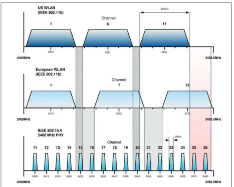
802.15.4 has 16 non-overlapping channels separated by 5 Mhz. Wi-Fi, Bluetooth and Zigbee all operates on 2.4 GHz. Figure2.5 shows the overlapping Wi-Fi and Zigbee
Figure 2.5: LR-WPAN vs Non-Overlapping WLAN Channel Allocations
channels. The interference by 802.11 can effect 802.14.4 given that the latter is narrow-band in comparison to the former. This interference can cause significant packet losses. Further, during one of the measurements, our sensor-testbed created problems for the other team. They informed us that our messages, reset their’s motes. Later, it was discovered that our initialization beacons were their reset commands. This means that MAC protocols cannot assume that they are the sole users of the channel. Therefore, analytical results in ideal system may not be applicable in the real-world systems.
Research community has put a lot of effort to study the effect of overlapping technologies, e.g., [50],[71],[85] and [86]. [85] concluded that effect of 802.11 on 802.15.4 can be negligible if the carrier frequencies of 802.11 and 802.15.4 are separated by at least 7 MHz. [50] concluded that 802.15.4 has minimal or no effect on 802.11 systems unless an 802.11 node is near a cluster of 802.15.4 nodes with very high activity.
While performing experiments for this thesis, we also do not observe any affect of the WiFi. We do observe interferences from the other Zigbee networks. Once our colleagues reported to us that their network was re-initialized when we started our network.
2.7. PROTOCOLS IN TINYOS 24
DSSS Transmission
As per the Jennic [56]’s technical report, IEEE 802.15.4 is designed to promote co-existence with other technologies. Therefore, the Direct Sequence Spread Spectrum (DSSS) transmit scheme is used for the communication. The basic idea is to use more bandwidth than is strictly required, thus spreading the signal over a wider frequency band. This is achieved by mapping the incoming bit-pattern into a higher data-rate bit sequence using a chipping code (effectively adding redundancy). Since the signal is spread over a larger bandwidth, narrow-band interferers block a smaller overall percentage of the signal, allowing the receiver to recover the signal.
2.7
Protocols in TinyOS
Collection Tree Protocol and MultihopLQI are the two collection protocols now available in TinyOS2.x . DRIP and DIP are the two dissemination protocols and finally the Deluge for over the air programming.
MultihopLQI [5]
• Mostly tested and used on platforms with CC2420. • Small footprint.
• Assumes links are symmetric. Collection Tree Protocol [42]
• System Independent. • Not thoroughly tested.
• Code foot print can be an issue. Drip [6]
• Fast and efficient for small number of items. • Trickle timers for advertisements.
DIP [7]
• Efficiently Disseminates large number of items (can not fit in one packet). • Use hashes and version vectors to detect and identify updates to the values. Deluge, [8]
• Over-the-air programming. • Disseminates code.
• Programs the nodes.
• If code size is large Deluge can not work.
2.8
MultihopLQI
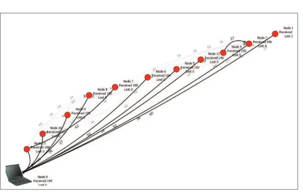
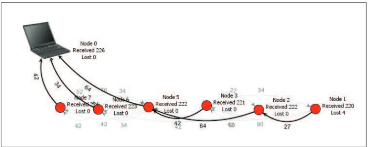
Figure 2.6: Sensornet
Figure2.6 exhibits an example of Ad hoc network, where nodes exchange some messages to construct their topology. MultihopLQI is the tree based routing algorithm. At the core of the algorithm is the use of routing beacons for a node to alert its neighbors about its current route to the destination. The MultihopLQI algorithms uses two types of messages:- 1). Data Message- set by the application layer 2.) Beacon Message- set by the