Department of Physics
University of Fribourg (Switzerland)
Synchrotron radiation based high–resolution grazing emission X–ray fluorescence
THESIS
presented to the Faculty of Science of the University of Fribourg (Switzerland) in consideration for the award of the academic grade of Doctor rerum naturalium
by
Yves Kayser
from
Luxembourg
Thesis No: 1717 Editor: UniFr – UniPrint
Prof. Dr. Christian Bernhard, Université de Fribourg (President of the jury) Prof. Dr. Jean–Claude Dousse, Université de Fribourg (Thesis Supervisor) Dr. Joanna Hoszowska, Université de Fribourg (Expert)
Dr. Burkhard Beckhoff, Physikalisch–Technische Bundesanstalt (External expert)
Fribourg, July 7th 2011
Thesis supervisor Dean
Abstract V
Résumé VII
Zusammenfassung IX
I. Introduction 1
II. Total Reflection X–ray Fluorescence 5
II.1. X–ray standing wave technique . . . 5
II.2. Total external reflection of X–rays . . . 8
II.3. Critical angle for total external reflection . . . 10
II.4. Characterization of the TXRF standing wave–pattern . . . 12
II.5. Standing wave–patterns of TXRF and XSW . . . 13
II.6. TXRF instrumentation . . . 16
II.7. Applications of TXRF . . . 21
III. Grazing Emission X–ray Fluorescence 29 III.1. Principle of microscopic reversibility . . . 29
III.2. GEXRF setup . . . 33
III.3. GEXRF applications . . . 37
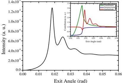
III.4. Intensity Calculations . . . 41
III.4.1. Theoretical derivation . . . 41
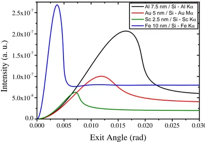
III.4.2. Examples . . . 48
IV. Experimental Setup 59 IV.1. ESRF ID21 beam line . . . 59
IV.2. Von Hámos spectrometer . . . 62
IV.2.1. Von Hámos geometry . . . 62
IV.2.2. Technical details . . . 67
IV.2.3. Realization of grazing emission conditions . . . 73
IV.3. High–resolution microfocused GEXRF . . . 76
IV.3.1. Polycapillary optics . . . 76
IV.3.2. Installation of a polycapillary optics in the von Hámos spec-trometer . . . 80
V. Experimental 91 V.1. Motivation for depth–profiling experiments . . . 92
V.2. Current methods for depth–profiling . . . 96
V.3. Experimental Conditions and Measurements . . . 100
V.3.1. Al–implanted Si wafers . . . 101
V.3.2. P–, In– and Sb–implanted Si wafers and P–implanted Ge wafers . . . 105
VI. Results and Discussion 111 VI.1. General Considerations . . . 111
VI.2. Theoretical Inversions . . . 114
VI.2.1. The truncated Laplace transform and Tykhonov’s regular-ization method . . . 115
VI.2.2. The maximum–entropy method . . . 119
VI.3. Fitting with a Gaussian . . . 121
VI.4. Fitting with joined half–Gaussian distributions . . . 126
VI.5. Fitting without a priori knowledge . . . 129
VI.6. Quantification and scan of the implantation homogeneity . . . 133
VI.7. Comparison to AES measurements . . . 134
VI.8. Comparison to GIXRF and SIMS measurements . . . 135
VII. Conclusion 141
List of Figures 145
References 153
Acknowlegements 167
Curriculum Vitae 169
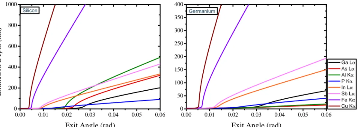
Photo–induced surface–sensitive X–ray fluorescence measurements can be realized by different means. One can either irradiate the sample with a collimated pri-mary X–ray beam at shallow incidence angles (0 to 2 degrees) relatively to the surface, or alternatively detect the X–ray fluorescence under well–defined shallow emission angles relatively to the sample surface. The first case corresponds to the Total Reflection X–ray fluorescence (TXRF) method, or the grazing incidence X–ray fluorescence (GIXRF) technique in the angle–dependent version, and the latter to the grazing emission X–ray fluorescence (GEXRF) technique. The prin-ciple of these methods is either to confine the X–ray fluorescence production to a surface–near region (on a nanometer scale) or to detect only the X–ray fluores-cence emitted by surface–near atoms. In both geometries the probed depth region, which extends from the sample surface into the bulk, changes significantly with the angle and varies from a few nm to several hundred nm.
The physical principles of TXRF, GIXRF and GEXRF will be thoroughly pre-sented. The requirements on the experimental setup for the realization of grazing incidence or grazing emission conditions, as well as their main differences, will be discussed. From a purely physical point of view the grazing incidence and the grazing emission geometry can be treated equivalently because of the principle of microscopic reversibility. Thus, their application domains are similar. In partic-ular, the variation of the probed depth region with the angle predestines these methods for non–destructive depth–profiling experiments. The depth distribution of the atoms is assessed from the dependence of the X–ray fluorescence intensity on the angle. In the present thesis, GEXRF depth–profiling measurements for different ion–implanted Si and Ge wafers with different implantation energies and fluences will be reported. The motivation for carrying out depth–profiling mea-surements and the description of existing methods will be presented. Calculations of the X–ray fluorescence intensity dependence on the grazing emission angle
re-ported in review articles of H.P. Urbach und P.K. de Bokx will also be summarized.
The experiments were carried out by means of the von Hámos crystal X–ray spec-trometer of the University of Fribourg installed at the European Synchrotron Ra-diation Facility (ESRF) ID21 beam line. Both the spectrometer and the beam line will be presented in detail. The realization of the grazing emission conditions in the von Hámos geometry will be explained. In the experiments, profit was made from the high resolution of the wavelength–dispersive detection setup and the advantages offered by synchrotron radiation. In addition, a focusing polycap-illary half–lens was installed in the spectrometer for micro–focused experiments permitting a local characterization of the sample. The necessary modifications, operational requirements and equipment for a successful implementation of the polycapillary optics in the von Hámos spectrometer will be presented.
In principle, the extraction of the depth concentration distribution of the im-planted ions from the angular intensity profile of an X–ray fluorescence line mea-sured by means of the presented experimental setup can be realized with different approaches. However, those based on purely theoretical concepts, discussed in detail, did not provide satisfactory results because of experimental intensity fluc-tuations (Poisson noise). Conversely, adopting the dopant depth distributions calculated with the SRIM (Stopping and Range of Ions in Matter) code, well– defined distribution functions for the implanted dopant atoms could be assumed and implemented in the fit of the angular intensity profiles to assess the dopant depth distribution. This approach provided accurate results in good agreement with theoretical expectations. In addition, an algorithm for the extraction of the dopant depth distribution without a priori knowledge has been developed. Its application to real data and its limits will be discussed. For few samples, compar-ative measurements with GIXRF and secondary ion mass spectrometry (SIMS) were performed. The retrieved depth profiles were found to be in good agreement with the depth profiles obtained with GEXRF. In summary, the synchrotron ra-diation based high–resolution GEXRF technique presented in this thesis, which can be optionally combined with focusing optics for the primary X–ray beam, is a powerful tool for extracting dopant depth profiles of ion–implanted samples.
Des expériences par fluorescence X sensibles à la région près de la surface de l’échantillon peuvent être réalisées de différentes manières. Une possibilité, connue sous les noms de TXRF (Total Reflection X–ray Fluorescence – fluorescence X par réflexion totale) ou GIXRF (Grazing Incidence X–ray Fluorescence – fluores-cence X sous incidence rasante) consiste à irradier l’échantillon avec un faisceau de rayons X collimé sous des angles d’incidence très petits (entre 0 et 2 degrés). Une autre alternative, dénommée GEXRF (Grazing Emission X–ray Fluorescence – Fluorescence X en émission rasante) est de mesurer la fluorescence X sous des angles d’émission très petits et bien définis. Le principe de base est soit de confi-ner la production de la fluorescence X à une région proche de la surface (sur une échelle nanométrique), soit de détecter uniquement la fluorescence X émise par des atomes situés près de la surface. Dans les deux géométries, la région étudiée s’étend de la surface de l’échantillon jusqu’à une profondeur variant entre quelques nano-mètres et quelques centaines de nanonano-mètres selon l’angle d’incidence ou d’émission.
Les principes physiques sur lesquels se basent les méthodes TXRF, GIXRF et GEXRF, les exigences imposées à l’instrumentation expérimentale ainsi que les principales différences entre les trois méthodes seront discutés en détail. D’un point de vue physique, l’incidence et l’émission sous angles rasants peuvent être traitées de manière équivalente à cause du principe de réversibilité microscopique. Les do-maines d’application étudiés sont donc similaires. En particulier, la variation de la profondeur étudiée en fonction de l’angle d’incidence ou d’émission prédestine ces techniques à la mesure non destructive de la distribution d’implants dans la pro-fondeur de l’échantillon. Dans cette thèse de doctorat, les profils d’implantation de différents ions introduits par implantation ionique avec différentes énergies et dif-férentes doses dans des échantillons de Si et de Ge ont été déterminés au moyen de la méthode GEXRF où la dépendance de l’intensité de la fluorescence émise par les atomes implantés est mesurée en fonction de l’angle d’émission. La motivation qui
nous a conduit à réaliser de telles mesures ainsi que les méthodes expérimentales alternatives existantes seront discutées. Un résumé du modèle théorique développé par H.P. Urbach et P.K. de Bokx pour calculer la variation de l’intensité de la fluo-rescence en fonction de l’angle d’émission sera également présenté.
Les mesures ont été réalisées en haute résolution avec le spectromètre à cristal incurvé von Hámos de Fribourg, lequel a été installé sur la ligne ID21 de l’ESRF (European Synchrotron Radiation Facility). Le spectromètre, sa géométrie, la réa-lisation des conditions d’émission rasante ainsi que la ligne de faisceau seront pré-sentés en détail. Les mesures ont pu être réalisées grâce aux avantages offerts par le rayonnement synchrotronique et la haute résolution du spectromètre. En plus une optique polycapillaire focalisante a été installée à l’intérieur du spectromètre pour réaliser des mesures avec un faisceau d’une taille latérale micrométrique ce qui a permis une caractérisation locale de l’échantillon. Les modifications du spectro-mètre requises pour l’installation du polycapillaire, les exigences pour l’alignement de ce dernier et l’instrumentation nécessaire seront expliquées.
L’extraction des profils d’implantation des ions à partir de la dépendance angulaire de l’intensité de la fluorescence X, mesurée à l’aide du dispositif expérimental men-tionné ci–dessus, peut être réalisée de différentes manières. Des approches basées sur la théorie seront présentées bien que celles–ci ne délivrent pas des résultats sa-tisfaisants à cause des fluctuations d’intensité expérimentale. Alternativement, en se basant sur des calculs effectués à l’aide du code SRIM (Stopping and Range of Ions in Matter), une distribution bien définie peut être supposée pour reproduire les mesures et retrouver ainsi la distribution en profondeur des dopants implan-tés. Cette approche a donné de bons résultats en comparaison avec les attentes théoriques. De plus un algorithme n’utilisant aucune connaissance a priori de la distribution en profondeur des ions mis à part un profil en forme en cloche a été développé. Son application aux mesures et ses limites théoriques seront discutées. Pour certains échantillons des mesures comparatives avec les méthodes GIXRF et SIMS (secondary ion mass spectrometry – spectrométrie de masse à ionisation secondaire) ont donné des résultats en bon accord avec les mesures GEXRF. Les résultats de cette thèse montrent que la technique GEXRF à haute résolution uti-lisant le rayonnement synchrotronique, avec l’option d’utilisation d’une optique focalisante, est un outil puissant pour la détermination non destructive des profils en profondeur de dopants introduits par implantation ionique.
Photoinduzierte Röntgenfluoreszenzanalyse kann zur Oberflächenanalyse von ben eingesetzt werden. Zwei Möglichkeiten hierzu sind die Anstrahlung der be mit einem Röntgenstrahl unter streifenden Einfallswinkeln bezüglich der Pro-benoberfläche und die Beobachtung der Fluoreszenzstrahlung unter streifenden Ausfallswinkeln. Im ersten Fall ist von Totalreflexions-Röntgenfluoreszenzanalyse (TXRF – Total Reflection X–ray fluorescence) oder Röntgenfluoreszenzanalyse unter streifendem Einfall (GIXRF – Grazing Incidence X–ray Fluorescence) die Rede, im zweiten Fall von Röntgenfluoreszenzanalyse unter streifendem Ausfall (GEXRF – Grazing Emission X–ray Fluorescence). Die dahinter stehende Idee ist entweder die Erzeugung der Röntgenfluoreszenz auf eine oberflächennahe Schicht (auf einer Nanometerskala) zu begrenzen oder nur die Fluoreszenzstrahlung von oberflächennahen Atomen zu detektieren. In beiden Fällen ändert sich die unter-suchte Probentiefe, die sich von der Oberfläche in die Probe hinein erstreckt, mit dem streifenden Winkel und kann je nach Winkel zwischen ein paar Nanometer oder mehreren hundert Nanometer variieren.
Die physikalischen Grundlagen von TXRF, GIXRF and GEXRF werden ausführ-lich diskutiert. Die Anforderungen an die Messapparatur um streifende Einfallswin-kel oder streifende AusfallwinEinfallswin-kel zu erzeugen werden erörtert, sowie die Unterschie-de zwischen beiUnterschie-den Messgeometrien. Von einem rein physikalischen Standpunkt können beide Messgeometrien, wegen des Prinzips der mikroskopischen Reversibi-lität, als äquivalent betrachtet werden. Dem zu Folge sind sich die Anwendungs-gebiete der Verfahren ähnlich. Insbesondere die Abhängigkeit der erprobten Tiefe vom Winkel prädestiniert die beiden Messmethoden für nicht destruktive Tiefen-profilmessungen. Die Verteilung der Atome, die die Fluoreszenzstrahlung emit-tieren, kann von der Winkelabhängigkeit der Intensität der Fluoreszenzstrahlung abgeleitet werden. In der vorliegenden Dissertation wurden Tiefenprofilmessungen mit Hilfe der GEXRF Geometrie für ionenimplantierte Si and Ge Proben
vor-genommen. Die Wichtigkeit von Tiefenprofilmessungen wird hervorgehoben und bestehende Alternativen werden diskutiert. Eine Zusammenfassung der von H.P. Urbach und P.K. de Bokx publizierten Berechnungen der Winkelabhängigkeit der Intensität der Fluoreszenzstrahlung wird ebenfalls dargestellt.
Die Messungen der Winkelabhängigkeit der Fluoreszenzstrahlung wurden mit Hil-fe des von Hámos Kristallspektometers der Universität Fribourg an der Strahllinie ID21 im ESRF (European Synchrotron Radiation Facility) vorgenommen. Das Spektrometer, dessen Geometrie, die Definition von streifenden Ausfallwinkeln in dieser Geometrie, und die Strahllinie werden vorgestellt. Die hohe Energieauflö-sung sowie die Synchrotronstrahlung boten einzigartige Vorteile für die Durchfüh-rung der Messungen. Zusätzlich wurde eine mikrofokussierende Polykapillaroptik im Spektrometer installiert um eine lokale Charakterisierung der Probe zu er-möglichen. Die notwendigen Änderungen am Spektrometer, die Anforderungen an die korrekte Ausrichtung der Polykapillaroptik, sowie die erforderliche Ausrüstung diesbezüglich werden visualisiert.
Die Rekonstruktion der Tiefenprofile der implantierten Atome kann aus der, mit Hilfe der eben erwähnten Messapparatur, beobachteten Winkelabhängigkeit der In-tensität der Fluoreszenzstrahlung mit unterschiedlichen Ansätzen verfolgt werden. Auf theoretischen Konzepten basierende Ansätze werden präsentiert, sie liefern allerdings keine zufriedenstellenden Resultate. Anhand der Berechnungen der Tie-fenprofile mit Hilfe des SRIM (Stopping and Range of Ions in Matter) Programms, konnte die Tiefenverteilung der implantierten Atome aus der Winkelabhängigkeit der Fluoreszenzstrahlungsintensität konstruiert werden. Es zeigte sich eine gute Übereinstimmung mit den theoretischen Erwartungen. Zusätzlich wurde ein Al-gorithmus entwickelt, der es erlaubt die Tiefenverteilung der implantierten Atome ohne a priori Annahmen aus den Messungen zu extrahieren. Die Anwendung des Algorithmus auf experimentelle Daten und die Validität der erhaltenen Resultate werden diskutiert. Darüber hinaus wurden für einige Proben komplementäre Mes-sungen mit Hilfe von GIXRF und Sekundärionen–Massenspektrometrie (SIMS) vorgenommen. Die erhaltenen Tiefenprofile entsprachen den GEXRF Messungen. Die in dieser Dissertation vorgestellte, auf hoher Energieauflösung und Synchro-tronstrahlung basierende, GEXRF–Technik (mit der Möglichkeit eine fokussieren-de Polykapillaroptik zu nutzen) ermöglicht die Durchführung von präzisen, nicht destruktive Tiefenprofilmessungen von ionenimplantierten Proben.
Introduction
X–rays, which have a wavelength between the wavelengths of UV radiation and gamma rays, were discovered in 1895 by W.C. Röntgen [1], a discovery for which he was awarded the Nobel prize in 1901, and are nowadays widely used for an-alytical aims in physics, chemistry, biology, archeology, geology and medicine of course. Indeed methods based on X–ray excitation and detection offer, due to the soft interaction of X–rays with materials in comparison with ion excitation, the advantage of non-consumptive analysis while at the same time requiring little sam-ple preparation. In comparison to other analytical techniques an operation under atmospheric pressure can be envisaged for hard X–rays. The combination of these advantages allows to integrate X–ray based analytical setups as an automatized, routine control in manufacturing processes.
X–ray analytical methods where X–rays are used in the detection channel are either based on X–ray scattering or X–ray fluorescence. Other analytical methods may use X–rays only in the excitation channel, like it is the case in Auger electron spectroscopy (AES) and X–ray photoelectron spectroscopy (XPS).
In X–ray scattering techniques, an X–ray beam is incident on the sample and the scattered radiation is measured as a function of the incidence angle, the scattering angle, the energy (elastic or inelastic scattering) and sometimes the polarization. Scattering experiments allow to deduce structural information from crystalline, powder (polycrystalline) or liquid samples. In this perspective X–rays are optimal since their wavelength is comparable to interatomic distances. For example X–ray diffraction (XRD) experiments enabled J. Watson and F. Crick in 1953 to deter-mine the DNA structure [2].
X–ray fluorescence, on the other side, is based on the excitation and detection of X–rays. The X–ray emission process can either be induced by particles (elec-trons, protons, ions) or by X–rays, resp. gamma rays, provided there is enough energy to excite the electrons in the atomic shells surrounding the nucleus. During the following de–excitation process, the excitation energy can be emitted in the form of an Auger electron or a fluorescence X–ray photon. The energy of both the Auger electron and the emitted X–ray photon, which is measured in X–ray fluo-rescence experiments, is characteristic for the considered element. Consequently, if the electron involved in the de–excitation process originates from a valence shell, X–ray fluorescence experiments are essentially used when the (quantitative) ele-mental or chemical analysis are the main goals.
However, if the intent is to realize surface–sensitive X–ray fluorescence measure-ments, the quite large penetration depths of the primary X–rays used to excite the fluorescence radiation are cumbersome (Fig. I.1). Alternatively particles could
0 1 0 0 0 2 0 0 0 3 0 0 0 4 0 0 0 5 0 0 0 0 . 0 0 . 2 0 . 4 0 . 6 0 . 8 1 . 0 A tt en u at io n D e p t h ( n m ) S i l i c o n 0 1 0 0 0 2 0 0 0 3 0 0 0 4 0 0 0 5 0 0 0 0 . 0 0 . 2 0 . 4 0 . 6 0 . 8 1 . 0 1 . 5 k e V 2 . 5 k e V 3 . 5 k e V 4 . 5 k e V 5 . 5 k e V 6 . 5 k e V 7 . 5 k e V D e p t h ( n m ) G e r m a n i u m
Figure I.1: Illustration of the intensity decay for X–rays penetrating Si
re-spectively Ge bulk samples at normal incidence. The X–ray beams penetrate quite deeply into the bulk, making surface–sensitive measurements (in the nanometer regime) difficult if not impossible due to the large background con-tribution (Compton scattering, Rayleigh scattering, X–ray fluorescence) from the bulk.
be used to excite the X–ray fluorescence since their penetration depths into the sample are much shorter. However, particle induced X–ray emissions require a high–vacuum setup to avoid the absorption of the particles in air and result in noisier X–ray spectra. Indeed particles have compared to X–ray photons a larger probability to multiply ionize atoms, which makes the quantitative interpretation
of the spectra more difficult due to the many satellite lines. In addition a quite noisy background radiation is induced due to the particle Bremsstrahlung pro-duced in the bulk target. Fluorescence radiation inpro-duced by photons on the other hand provides cleaner experimental spectra which is especially useful in the case of micro- and trace analysis. The realization of surface–sensitive measurements is also possible by either adjusting the angle of incidence of the primary photon beam or the emission angle of the fluorescence radiation.
Total Reflection X–ray
Fluorescence
Usually the efficiency of surface analysis (or interface analysis of multilayered sam-ples) by means of X–ray probing is limited by the rather large penetration of the incident primary X–rays into the sample. The surface–near region is not efficiently excited with respect to the bulk. The excited fluorescence X–ray signal originates from the whole excited sample region and therefore the signal from the surface (or interface) region may be hidden in the bulk fluorescence signal or background (due to elastic scattering, detector noise and photoelectron Bremsstrahlung) if the X–ray energy of the surface elements is not located in a clean, i.e., free of any other signals, region of the X–ray spectrum.
One possibility to improve the surface analytical capabilities is to enhance the excitation of the atoms at the surface with respect to the excitation of bulk atoms. This can be done by creating an X–ray standing wave–pattern resulting from the coherent superposition of two plane waves on the surface of the bulk sample. To this end one can employ the X–ray standing waves (XSW) technique (Fig. II.1) or the total reflection of X–rays (Fig. II.2) as used in the total reflection X–ray fluorescence (TXRF) method.
II.1
X–ray standing wave technique
The XSW technique has been pioneered by B.W. Batterman [3] who used it to trace interstitial impurities in crystalline samples. The bulk sample is a perfect crystal or a multilayer and the standing wave–pattern results from the
interfer-D i f f r a c t e d P l a n e X - r a y W a v e d d P la n es w ith c o n str u ct iv e i n te rf er en ce I n c i d e n t P l a n e X - r a y W a v e S u r f a c e n n
Figure II.1: X–ray standing wavefield created by the interference of an
in-cident and a Bragg–diffracted (section IV.2.1) plane wave of wavelength λ around the surface region of a Bragg diffraction crystal. The maximum and minimum amplitudes of the plane waves are colored in blue, resp. in red. The planes in which constructive interferences take place are parallel to the Miller planes of the crystal and the periodicity is connected to the crystal lattice spacing.
ence of the incident X–ray beam with the Bragg diffracted beam (Fig. II.1). The condition for Bragg diffraction is discussed in paragraph IV.2.1, illustrated in Fig. IV.4 and mathematically described in Eq. IV.1 1. The theoretical description for the standing wave–pattern due to the coherent superposition of the incident and diffracted beams is based on the dynamical diffraction theory. The standing wave–pattern is characterized by regions with constructive, respectively destruc-tive, interference. The interference regions are parallel to the crystal Miller planes. In regions with constructive interference, the initial amplitude of the plane waves is doubled. The probability to excite fluorescence X–rays is increased compared to a situation where no interference effects take place, favoring thus the detection of X–rays emitted from the parts where constructive interference occurs. In re-gions with destructive interference the probability of photoelectric absorption is drastically reduced. By the different incidence angles around the Bragg angle, the
1Note that the Bragg law is for the constructive interference of plane X–ray waves diffracted at
different Miller planes of the crystal. The waves considered in this type of interference propagate therefore in the same direction in contrast to the waves creating the standing wavefield–pattern. The Bragg law assumes that phase differences between the diffracted waves are only due to different pathlengths, the phase shift upon the coherent scattering at the atoms of the Miller planes having a constant value.
standing wave–pattern is altered and accordingly the regions with constructive or destructive interference are displaced. This allows in principle to obtain spatial information on the distribution of the target element. This technique can also be combined with X–ray diffraction.
In the perspective of surface analysis, a drawback of the XSW technique is the extension of the standing wave–pattern which is formed both above and below the sample surface. A contribution from the bulk sample in the experimental X– ray spectrum is still present. If the focus of the experiment is surface analysis, a standing wave–pattern which is present only above the surface would be preferable since then only contributions from the region of interest would be present in the measured X–ray spectrum. In this perspective the penetration of the incident X– rays into the sample should be minimized. The total external reflection of X–rays on a smooth sample surface does not allow an X–ray photon to penetrate deeply into the sample, while at the same time a standing wave–pattern is created on top of the sample surface due to the interference of the incident and reflected X–ray beams (Fig. II.2).
R e f l e c t e d P l a n e X - r a y W a v e D P l a n e s w i t h c o n s t r u c t i v e i n t e r f e r e n c e i i I n c i d e n t P l a n e X - r a y W a v e S u r f a c e
Figure II.2: X–ray standing wavefield created by the interference of an
inci-dent and a totally reflected (section II.2) X–ray plane wave of wavelength λ. The maximum and minimum amplitudes of the plane waves are again colored in blue, resp. in red. The planes in which constructive interference takes place are parallel to the sample surface. The periodicity varies with the incidence angle θi and is larger than in the case of an X–ray standing wave–pattern created by Bragg diffraction (section II.5).
II.2
Total external reflection of X–rays
As X–rays are electromagnetic waves, refraction (transmission and reflection) of X–rays at the interface between different media takes place. The TXRF method is based on the total external (to the bulk sample) reflection of the incident X–ray beam, meaning that the reflected beam has an intensity nearly equal to the one of the incident beam and no refracted beam penetrates deep into the sample. A.H. Compton was the first to report in 1923 on total reflection of X–rays from solid samples [4], whereas the first theoretical formalism on the basis of dispersion the-ory was established by L.G. Paratt in 1954 [5] to discuss surface properties of solids.
In order to observe total reflection of X–rays (or light in general) at the inter-face of two media, two conditions need to be satisfied:
1. The refractive index n1 of the medium in which the X–ray beam is initially propagating needs to be larger than the refractive index n2 of the medium onto which the beam is incident. The second medium should be optically less dense.
2. The X–ray beam should be incident on the interface at angles θi below the critical angle for total reflection.
Both conditions can be derived from Snell’s law (also known as Snell–Descartes law) which can be deduced from the continuity condition for the incident, reflected and refracted electromagnetic waves at the interface requiring that the temporal and spatial evolution of the three waves shall be identical at the interface,
n1× cos θi = n2× cos θt. (II.1)
In the case where n1 > n2 with an X–ray beam incident from the medium with refractive index n1 on the medium with refractive index n2, i.e., in a situation cor-responding to the first condition for total reflection, the refraction angle θt needs to be smaller than θi in order for Eq. II.1 to be verified. This means that upon penetration into the second medium with refractive index n2 the X–ray beam is refracted towards the interface of the two media (Fig. II.3). Accordingly there exists a minimum angle θi for which θt = 0◦, meaning that the refracted X–ray beam propagates along the surface in medium 2. This angle is called the critical angle for total reflection θc = arccos(n2/n1), the incident beam cannot be further
r e f l e c t e d r e f r a c t e d 2 2 2 1 1 1 n 1 n 2 i n c i d e n t i n c i d e n t r e f l e c t e d r e f r a c t e d
Figure II.3: At the interface between two media of refractive indexes n1
and n2, with n2 < n1 in the present example, light beams in general and
X–ray beams in particular are partially refracted (transmitted) and partially reflected. The reflection angle is equal to the incidence angle θ1on the interface while the refraction angle θ2 and thus the deviation of the refracted beam is fixed by Snell’s law (Eq. II.1).
refracted towards the interface boundary for incidence angles θi smaller than θc (section II.3). Indeed only an evanescent, exponentially damped wave, propagating along the surface penetrates into the second medium. The short, vertical pene-tration range is due to energy and momentum conservation. The incident beam will be reflected, the reflection angle θr being identical to the incidence angle θi (Fig. II.3) because of the continuity condition at the interface. This justifies the second condition for total reflection. The incident and reflected beam will super-pose coherently above the region where the incident beam hits the sample surface, creating a standing X–ray wave–pattern (Fig. II.2).
The total external reflection of X–rays not only improves the excitation efficiency for fluorescence radiation of the near–surface region like the XSW technique does but prevents in addition any fluorescence excitation of the bulk, provided the in-cidence angle θi is below the critical angle for total external reflection θc (see Fig. II.4). For larger incidence angles θi, the primary X–ray radiation can penetrate into the sample, but due to the shallow incidence angles, the X–ray absorption is quite pronounced in the depth direction (factor sin θi), limiting the depth region which is effectively excited to very narrow regions (see Fig. II.4 and Fig. I.1 for comparison).
For n1 < n2 no total reflection can occur, since the refracted beam will be re-fracted away from the interface of the two media and will therefore penetrate into the medium with refractive index n2, independently of the incidence angle θi (Fig. II.3).
0 . 0 0 0 . 0 1 0 . 0 2 0 . 0 3 0 . 0 4 0 . 0 5 0 . 0 6 0 2 0 0 4 0 0 6 0 0 8 0 0 1 0 0 0 G e r m a n i u m I n c i d e n c e A n g l e ( r a d ) 1 . 5 k e V 2 . 5 k e V 3 . 5 k e V 4 . 5 k e V 5 . 5 k e V 6 . 5 k e V 7 . 5 k e V 0 . 0 0 0 . 0 1 0 . 0 2 0 . 0 3 0 . 0 4 0 . 0 5 0 . 0 6 0 2 0 0 4 0 0 6 0 0 8 0 0 1 0 0 0 S i l i c o n E x ti n ct io n D ep th ( n m ) I n c i d e n c e A n g l e ( r a d )
Figure II.4: Plot of the extinction depth as a function of the incidence angle
θi for different primary beam energies in Si and Ge. The extinction depth
corresponds to the perpendicular distance from the surface after which the intensity has been attenuated by a factor e−1. The extinction depth depends strongly on the incidence angle θi: below the critical angle θc (marked by a
steep step in the variation of the extinction depth) only a shallow surface layer (about 3–5 nm) is penetrated, whereas for larger incidence angles the primary X–rays penetrate deeper into the sample. However, in comparison to Fig. I.1, the extinction depth is much narrower for grazing incidence angles.
II.3
Critical angle for total external reflection
Since the refractive index n1 of vacuum is one, the condition for total external reflection of X–rays incident on the sample with refractive index n2can be rewrittencos θc= n2/n1 = n2. (II.2)
The refractive index of solid samples in the X–ray domain is a complex quantity, n2 = 1 − δ2 + iβ2, the refractive index decrement δ2 and the absorption index β2 being positive quantities related to the scattering and absorption properties [6],
δ2 = NA 2π × re× ρ2 A2 × f2(λi) × λ2i, (II.3) β2 = µ2(λi) 4π × ρ2× λi. (II.4)
Here λi represents the wavelength of the incident X–rays, NA = 6.022 × 10²³ the Avogadro’s number, re = 2.818 × 10⁻³ Å the electron radius (or equivalently the X–ray scattering amplitude per electron), ρ2 the mass density of the scattering sample, A2 the molar mass of the sample, µ2(λi) the total mass absorption coeffi-cient of the sample’s element and f2 = f2(0) + f2∗(λi) the real part of the atomic scattering factor, where f2(0) corresponds to the atomic forward scattering fac-tor, being approximately equal to the atomic number Z2 of the sample’s element
(the difference being given by a small relativistic correction [7]) and f2∗(λi) to a correction factor that is essential in the X–ray wavelength domain below the ab-sorption edges of the sample’s element. In formulas II.3 and II.4 a homogeneous monoelemental sample was assumed but the formulas can also be applied if the scattering factor f2 is known for the considered compound, the other factors being in principle calculable with a weighted linear combination of the corresponding elemental factors. The weights are given by the relative elemental concentration. The ratio NAρ2/A2 corresponds to the atomic density, which can be related with f2(0) to the electronic density, the electrons being the X–ray scatterers.
The order of magnitude of δ2 and β2 varies between 10−3 and 10−6. The real part of the refractive index n2 is thus really close to one, implying that θc is very small. Representing the cosine function by the first terms of a Taylor series one obtains: n2 = cos θc ≈ 1 − θ2 c 2 ⇒ θc ≈ q 2 × δ2 ≈ λi √ π × s NA× re× ρ2× Z2 A2 . (II.5)
The latter approximation is for X–ray wavelengths shorter than wavelengths cor-responding to the absorption edges of the sample’s element. Given the order of magnitude of δ2, the critical angle θc for total external reflection is of the order of 1◦ or smaller. It depends on the sample’s element and the wavelength of the in-cident X–rays and tends to decrease for heavier elements and higher X–ray energies.
In order for total external reflection to happen, i.e., the reflection occurs on the vacuum (or air) side of the vacuum (resp. air) – sample interface for a bulk sam-ple, the refractive index of the sample (the second medium) should be smaller than one, the refractive index associated to vacuum (resp. air). This premise is valid for solid samples in the wavelength domain of X–rays, as explained in [6] and [8] with the following arguments. The X–ray frequency is of the order of the binding frequency of the atomic electrons. In the derivation of the refractive index n in the Lorentz theory, the electrons are assumed to be quasi–elastically–bound and forced to oscillations by the incident primary X–rays. Upon this the electrons radiate with a phase–difference and by superposition of both radiations the phase velocity v of the primary beam is altered to values larger than c, the speed of light. Hence the refractive index n = c/v is modified to values smaller than one
by a quantity δ. This is not in contradiction with the relativity theory, since the group velocity, i.e., the speed at which the signal is transported, does not exceed c.
The refraction angle is a complex number and can also be calculated with Eq. II.1 with the small angle approximation for the cosine functions,
θt= v u u t θ2 i − 2 × δ2+ 2i × β2 1 − δ2+ iβ2 (II.6)
For visible light, only total internal reflection, on the sample side of the air–sample interface, can occur since in this wavelength region the refractive index of a solid sample is always larger than one.
II.4
Characterization of the TXRF standing wave–
pattern
The sample surface is supposed to be perfectly smooth on the nanometer scale. The X–ray standing wave–pattern is formed on top of the sample surface by the coherent superposition of the incident X–ray beam ~E1(~r, t) with the one reflected by the sample surface ~E2(~r, t),
~
E(~r, t) = E~1(~r, t) + ~E2(~r, t)
= E~0× exp i(ωt − ~k · ~r) + ~E0R× exp i(ωt − ~kR· ~r + ∆φR), (II.7) where ER
0 is the amplitude of the reflected beam and E0 the amplitude of the incident beam, ~k the wavevector with norm k = 2π/λi = kR and ∆φR the phase difference between the incident and the reflected plane X–ray wave due to scatter-ing. The transmitted plane wave is defined similarly to the incident and reflected plane waves,
~
E3(~r, t) = ~E0T × exp i(ωt − ~kT · ~r + ∆φ
T), (II.8)
the norm of the transmitted wavevector being kT = n
2× 2π/λi. The reflectivity R and transmittivity T are defined as
R = ER 0 E0 2 and T = ET 0 E0 2 . (II.9)
Assuming a reflectivity R equal to 1, i.e., total reflection, and requiring the spatial and temporal evolution of the incident and the sum of the refracted and transmit-ted vectors to be identical at the surface, the wavevectors ~k and ~kR are collinear
and the total electromagnetic vector ~E(~r, t) resulting from the superposition will be equal to ~ E(~r, t) = ~E0cos (~k − ~kR) · ~r 2 + ∆φR 2 × exp i(ωt − (~k + ~kR) · ~r 2 + ∆φR 2 ).(II.10)
Choosing a coordinate system with the z axis perpendicular to the surface and pointing out from it, z = 0 corresponding to the sample surface which lies thus in the xy–plane, and assuming the incident wavevector ~k to be confined in the xz–plane, Eq. II.10 gives for a plane wave incident at the angle θi relative to the surface
~
E(~r, t) = ~E0cos (k sin θi× z + ∆φR
2 ) × exp i(ωt − k cos θi× x + ∆φR
2 ). (II.11)
This result corresponds to a wavefield moving along the x–direction but presenting standing waves in the z–direction. Parallel to the surface there are nodal and anti– nodal lines with zero or maximum amplitude, respectively, meaning that the cosine function has either the value zero or unity. The period, or spacing, of the nodal or anti–nodal lines is given by the periodicity of the cosine function and is equal to λi/2 sin θi. The intensity in the general case where the reflectivity is not one is given in [9] I(θi, z) = |E0|2× 1 + R + 2 √ R × cos arccos(2θ 2 i θ2 c − 1) − 4πz sin θi λi !! .(II.12)
The maximum and minimum values of I(θi, z) define the anti–nodal and nodal lines, respectively.
Below the surface the intensity is exponentially damped due to X–ray absorption, the beam propagating along the direction defined by θt (Eq. II.6). The surface (z = 0) intensity is defined by Eq. II.12 since the intensity varies continuously [6].
II.5
Standing wave–patterns of TXRF and XSW
Both Bragg diffraction used in the XSW technique and total external reflection of X–rays used in the TXRF method can be employed to create standing X–ray wavefields of monochromatic, coherent X–ray beams propagating in different di-rections. As it has been mentioned, in the first case the coherent scattering of X–rays at the atoms of the different crystal planes is used, while in the secondcase the total external reflection of X–rays at a perfectly smooth vacuum–sample interface is employed. Therefore a few differences result in the properties of the standing X–ray wave–pattern. The first one concerns the samples. For the XSW technique only crystals are used, whereas for the TXRF technique any sample with a smooth (on the nanometer scale), homogeneous and sharp vacuum–sample interface is conceivable. However, samples with low–Z elements are preferred since they offer larger critical angles θc and are therefore less demanding in the angular alignment to achieve total external reflection conditions.
Another difference is the period between regions with constructive interference in the X–ray standing wave–pattern. For a standing wave–pattern created by means of the XSW technique, the period is determined by the lattice spacing between the Miller planes of the crystal and is therefore of the order of a few Ångström. When the TXRF method is used, the period is a strong function of the incidence angle θi and, referring to Eq. II.11, varies as [9]
D = λi 2 sin θi
. (II.13)
The periodicity can also be geometrically deduced from Fig. II.2. As a conse-quence, the period in the standing wave–pattern is much longer in the latter case due to the small angles of incidence θi. Thus, standing wave–patterns created by means of total external reflection are more suitable for the analysis of impurities in layers thicker than a few Ångström. Indeed there will be no ambiguity due to the very short period of a standing wave–pattern created by means of Bragg diffrac-tion [9], which allows nevertheless to very accurately localize adsorbate atoms on crystal surfaces [10,11]. In the TXRF case the period of the standing wave–pattern will vary from infinity at 0◦ incidence angle to
Dcrit.= λi 2 sin θc ≈ λi 2θc ≈ λi 2√2δ2 = √ π 2 × s A2 NA× re× ρ2× Z2 (II.14)
at the critical angle θc. Note that the latter value is independent of the incident X–ray wavelength λi and depends solely on the reflecting sample.
The boundary condition at the vacuum–sample interface implies that in the case of total reflection the phase shift between the incident wave and the reflected wave varies from π to zero if the incidence angle θi varies from 0◦ to θc. This means that at 0◦ the nodes of the wave–pattern lie on the sample surface and at the
critical angle θc the antinodes. The nodes correspond to the regions with destruc-tive interference where the phase difference between the incident and reflected (or diffracted) beam corresponds to an odd multiple of π. Equivalently, in the antin-odes the phase difference is an even multiple of π and constructive interference occurs. At the antinodes, the amplitude of the total wavevector (i.e., the sum of the incident and reflected wavevectors) is doubled and the intensity is multiplied by four (see Eq. II.12, assuming a reflectivity of 100%).
In the Bragg diffraction case, the conditions to fix the phase of the diffracted beam are more complex [10]. However, an angular scan through the Bragg region, i.e., the region in the vicinity of the Bragg angle, corresponds to a phase shift of π or equivalently to a shift of the nodal and anti–nodal lines by half of the lattice spacing d (into the crystal if the scan is performed from smaller to larger incidence angles). For the smallest angle the nodal lines and for the largest angle the anti– nodal lines are on the diffracting Miller planes. The nodal and anti–nodal lines present not only a periodicity corresponding to the crystal lattice spacing d but they are also parallel to the crystal Miller planes. Outside the Bragg region, the modulation of the wavefield is lost as the intensity of the diffracted beam decreases strongly [12]. In the TXRF case these lines are parallel to the surface. For both techniques the standing X–ray wave–pattern can be altered by an angular adjust-ment of the monochromatic incident X–ray beam: in the XSW case it is shifted, in the TXRF case it is compressed (when D decreases) or decompressed (when D increases).
The bulk background contribution to the experimental result is lower if the stand-ing wave–pattern is created by TXRF than if it is produced by Bragg diffraction. On one side there is the peak reflectivity which can approach 100% in the total reflection case for perfect metallic mirrors but is usually lower for Bragg crystals. On the other side, there are geometrical considerations. In the TXRF approach, the evanescent wave propagation along the sample surface affects a narrower region than in a Bragg crystal irradiated at the Bragg angle. Nevertheless in both cases, the background contributions can be drastically reduced by tuning the wavelength λi of the incident X–ray beam above the absorption edge wavelengths of the bulk atoms (if the latter are below the absorption edges of interest for the experiment). The surface regions over which the standing wave–patterns extend vary inversely with the incidence angle θi and are thus larger in the total reflection regime for
identical beam widths. However, the X–ray source coherence lengths have also a major impact on the extension of the standing wave–pattern, especially in the height direction (along the z–axis) [13, 14].
II.6
TXRF instrumentation
The geometry of a TXRF setup corresponds to a special configuration of an energy– dispersive X–ray fluorescence (EDXRF) setup [15], the difference being the stand-ing X–ray wave–pattern created in front of the sample. While for EDXRF the beam intensity in front of the sample surface has a constant value, it is charac-terized by local oscillations in the TXRF case (see Eq. II.12). The oscillations vary between zero and four times the intensity of the incident beam for a per-fectly reflecting surface. Thus, in comparison to EDXRF, the fluorescence signal of particles above the surface is considerably enhanced since the probability for a photoelectric absorption is correspondingly locally enhanced. At the same time the background contribution is drastically reduced. Indeed, for typical TXRF in-cidence angles θi below the critical angle θc, only an evanescent wave penetrates a few nanometers into the sample (Fig. II.4), while in a standard EDXRF setup the primary beam penetrates up to a few micrometers into the sample (Fig. I.1). As a consequence a TXRF setup presents a drastically improved signal–to–background ratio compared to EDXRF.
Since TXRF is a special case of EDXRF, the instrumentation for measurements is similar, except that there are a few special requirements on the primary beam and the sample surface. Basically the setup for TXRF measurements consists of an X–ray source, a beam modulation unit, the sample with its holder and an energy– dispersive detector [6, 16–18] (Fig. II.5). In the choice of the setup components presented hereafter a difference needs to be made, depending on the purpose of the measurement [6].
1. If, for example, the aim is to check the quantitative elemental composition of grains or residues on top of a reflecting surface, measurements at a single, fixed incidence angle θi below the critical angle θc will be sufficient. Usually an incidence angle θi of about 71% of the critical angle θc is chosen. This incidence angle is called the isoradiant angle in [19].
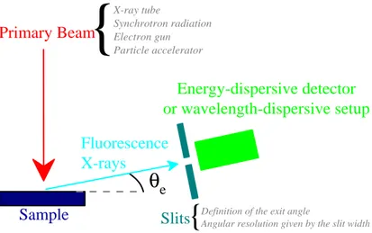
E n e r g y - d i s p e r s i v e D e t e c t o r θi X - r a y f l u o r e s c e n c e r a d i a t i o n X - r a y s o u r c e S a m p l e B e a m M o d u l a t i o n U n i t C o l l i m a t e d P r i m a r y X - r a y B e a m P o s ition in g
Figure II.5: Schematic view of the main components of a TXRF–based setup:
the X–ray source which can be an X–ray tube or a synchrotron light source, the beam modulation unit for geometrical (and monochromatic) refinement of the X–ray beam, the sample, which in GIXRF setups can be oriented relatively to the beam, and the energy–dispersive detector for the measurement of the fluorescence X–rays. Details can be found in the text.
in–depth distribution of (buried) layers, for example, then the fluorescence intensity needs to be recorded at different incidence angles θi (below and also above the critical angle θc). Here a monochromatic incidence beam is required to avoid to blur the correlation between the standing wave–pattern and the local distribution of the fluorescence atoms.
These experimental requirements affect especially the beam preparation and sam-ple positioning system. Experimental setups optimized for the first type of exper-iment are called TXRF setups, while for the second type of experexper-iment they are called grazing incidence X–ray fluorescence (GIXRF) setups.
The X–ray source
The X–ray source may be a high power, fine focus X–ray tube with a fixed or rotating anode or a synchrotron radiation beam line. Only these two types of X– ray sources provide high enough intensities to realize measurements in a reason-able time interval. A synchrotron radiation beam offers the additional advantages of energy–tunability, monochromaticity, linearly polarization and low divergence. This reduces the requirements on the beam modulation unit.
The beam modulation unit
After the source the spatial shape and spectral distribution need to be refined. The beam incident on the target should be indeed a few micrometer high, the height being the vertical direction with respect to the propagation direction. For
reasons of angular resolution of the incidence angle, the beam divergence in the vertical direction should be very low. The width may be a few millimeter up to one centimeter and is mainly limited by the detector window’s dimensions for easier quantification. A first refinement of the geometrical beam shape can be realized with collimator slits or metallic edges acting as diaphragms.
The refinement of the spectral distribution when an X–ray tube is used depends on the aforementioned experimental purposes. In the case of elemental quantification, it is sufficient to remove the high–energy part of the continuous Bremsstrahlung. Indeed Eq. II.5 shows that the critical angle θc depends inversely on the X–ray energy. Consequently total reflection conditions are more difficult to realize for high X–ray energies. Since the photoelectric cross–section diminishes also with the energy and as the high–energy part of the continuous Bremsstrahlung spec-trum contains only a small fraction of X–ray photons (Fig. II.6), it is removed from the incident beam by a low–pass filter. The low–pass filter can be a either
0 1 0 2 0 3 0 4 0 0 . 0 0 . 2 0 . 4 0 . 6 0 . 8 1 . 0 N o rm al iz ed I n te n si ty ( a. u .) E ( k e V )
Figure II.6: Theoretical example for the continuous Bremsstrahlung
distri-bution of an X–ray tube. In this example a W anode, a voltage of 40 kV and a 150 µm thick Be window were chosen. The characteristic lines (Lα at 8.398 keV, Lβ at 9.672 keV and Mα at 1.775 keV) of the anode are omitted.
metallic mirror or a perfect crystal or glass upon which the geometrically refined beam is incident at a grazing angle, called the cut–off angle θcutwhich depends on the selected cut–off energy Ecut (Eq. II.5). X–ray photons with a higher energy than the cut–off energy Ecut are not totally reflected and thus removed from the beam by absorption in the low–pass filter. To diminish the divergence of the beam and sharpen the cut–off in its spectral distribution, the beam may be multiply reflected, at the expense of a lower intensity. If the experimental purpose is the assessment of the elemental spatial distribution by a scan of the incidence angle θi, the spectral distribution needs to be adjusted by a monochromator to produce a monochromatic beam. For X–ray tubes this means that the characteristic
flu-orescence lines of the X–ray tube anode are to be used since the latter provide the highest X–ray intensities. For synchrotron radiation the choice of the primary X–ray energy is far less restricted. Different setup configurations or categories to modulate the beam are mentioned in [17]. In any setup it is essential that a (monochromatic) low–divergence beam is produced by the beam modulation unit.
The sample and its positioning
The incidence angle θi of the beam is controlled by positioning the sample ade-quately. The specific requirements on the sample positioning system depend on the experimental purpose. For elemental quantification with a laboratory X–ray tube and a fixed beam modulator unit where a single measurement at a fixed incidence angle is sufficient, the sample may simply be pressed against a reference holder to adjust the incidence angle θi. Otherwise a 5–axis motorized sample position-ing system with 3 translational and 2 rotational (around the axes of the surface) displacement directions is necessary. The incidence angle θi needs to be known precisely and varied accurately. Geometrical effects due to the varying incidence angle are discussed in [20].
The reflecting surface on which the residues or grains are disposed, respectively the (layered) sample surface, have also to meet some requirements. Ideally it should be characterized by a high reflectivity R (to reduce the scattered background radi-ation), a very low roughness and the absence of waviness within the irradiated area in order to meet the requirement of being optically flat and smooth and presenting a sharp, plane vacuum (air) – sample boundary (section II.4). The requirements of sharp interface boundaries hold also for the layers of a layered sample; in ad-dition the boundaries should be parallel to the surface so that the properties do not vary in a plane parallel to the surface. The effects of rough surfaces or layer interfaces in the grazing incidence geometry are widely discussed in literature and introduced in theory [21–28]. In the case of trace analysis with a typical TXRF setup, the carrier of the residues or grains should also be free of impurities and resist to cleaning with acids. Different types of glass carriers or pure crystals may assume the role of a carrier. At the same time the residue or grain size should be sufficiently small to not disturb the X–ray standing wave–pattern created on top of the reflecting surface [29].
The X–ray fluorescence detector
The excited X–ray fluorescence signal is detected by an energy–dispersive detector mounted close (about one centimeter) to the sample surface. The small distance between the detector and the sample surface ensures a large solid angle of de-tection and thus an efficient X–ray fluorescence signal dede-tection, permitting to reduce the counting time. Different orientations of the detector with respect to the sample surface have been compared in [30] to find the best configuration. The use of a synchrotron radiation beam permits to reduce the background related to scattering. Aligning the sample surface along the linear polarization vector of the synchrotron beam diminishes indeed the scattered X–ray intensity in the detector direction [31]. Energy–dispersive detector present also the advantage of simultane-ous multi–elemental detection, even if they suffer from a lower efficiency for X–rays emitted by low–Z elements. In this energy range the energy resolution, of about 130 eV for the best detectors, and escape peaks may be also troublesome.
The sample–detector assembly can be operated in air, a huge advantage with respect to other surface–analytical techniques. To reduce the absorption, a He en-vironment may be advantageous. To further diminish the absorption effects, the whole setup can be placed in vacuum. This allows to use windowless detectors for a better detection of the X–ray fluorescence signal emitted by low–Z elements.
Developments
The different parts of TXRF setups have profited over the years from on–going technical developments and improvements. Profit was made of X–ray tubes with increased intensities and more efficient X–ray optics until physical limits were reached [32]. Detectors with improved signal–to–background ratios and better resolutions were made available. The advent of synchrotron radiation sources pro-vided very intense X–ray sources. However, the increased source intensity results not only in an increased X–ray fluorescence intensity but also an increased back-ground radiation from the sample with the risk to overload the detector. Detectors supporting high count rates, i.e., detectors with very low dead and shaping time are thus necessary to profit from the increased source intensity, the alternative being a decrease of the solid angle of detection. Silicon drift detectors (SDD), supporting count rates of up to 106 counts per second have nowadays replaced the Si(Li) detectors if a very bright X–ray source is used [16].
Different designs for the beam modulator unit were tested [33–35] and the use of polycapillary optics in the collimation direction [36], respectively the focusing direction, together with slits [37], was proposed instead. More details on polycap-illary optics can be found in section IV.3.1.
II.7
Applications of TXRF
The TXRF experimental conditions at glancing incidence angles below the critical angle θc are characterized by a surface reflectivity close to 100% and a penetration depth of a few nanometers in the in–depth direction of the sample. Thus the main applications of the TXRF method are the surface and near-surface analysis of samples. Compared to standard X–Ray fluorescence (XRF) measurements, TXRF experiments profit from the significantly improved sensitivity, due to the more efficient excitation and drastically reduced background, for elemental detection at the sample surface region while preserving at the same time the advantages of being non–destructive, applicable to a wide range of materials and not very time consuming [15]. Another good point for TXRF compared to some other trace analysis methods is the possibility to regroup the different components in a compact laboratory spectrometer. This promoted the use of TXRF setups.
Elemental micro- and trace–analysis
One of the main applications of TXRF is (quantitative) micro- and trace–element analysis. TXRF was already used in this perspective in the late 1980’s [38,39] and then promoted in the early 1990’s as an efficient tool in this domain [40]. The quantification is realized by adding a well-known quantity of a reference element to the sample, in order to assess the detection efficiency; afterwards the different detected elements can be quantified with respect to the reference [13], the broad linear range of 3–4 orders of magnitude of the detectors being advantageous [16]. A drawback is that the sample mass needs to be known. Sampling techniques for TXRF are reported in [41]. Usually a small sample amount is deposited (either in the form of small grains or a droplet which is dried before the experiment) on a re-flecting surface, the reflector, and irradiated at a fixed incidence angle θi below the critical angle θcdetermined by the reflector and the (shortest) wavelength λi of the incident X–rays. The experimental purposes are twofold, either the quantitative
el-emental composition of a sample or the presence of contaminants in or on a sample has to be assessed. In this perspective TXRF is used in a wide range of domains: in medicine for the analysis of human blood, blood serum or human hair [42–45] and the analysis of human tissues [46–50], in pharmacy to analyze drugs [51,52], in petrochemistry [53, 54], in food science to detect harmful elements or to assess the environmental influences [55–60], in biology [61], in life sciences [62], in forensic sciences [63], in soil analysis and environmental sciences [64–67], in the analysis of materials used at nuclear plants [68], in archeology [69–72], in cultural heritage studies [73–76] and in the study of ancient artworks and historical objects [29].
Especially in the latter domains the micro- and trace–analytical capabilities prove to be useful. Indeed minute sample amounts are sufficient for the analytical pur-poses and the acquisition of reliable results. An overview of the sample preparation methods is presented in [13], where it is shown that special care is necessary for the homogenization of the sample. The advantage is that the object of study remains almost unaltered and is thus preserved. The sample does not need to be displaced, nor does the detection setup. Thus the analysis is completely non–destructive, the representativeness of the results obtained with very small sample pieces compared to the object of study remaining, however, questionable in some cases.
Surface contamination control
The most successful micro- and trace–analysis application with regard to industrial applications is, however, the detection of contaminants on semiconductor wafers which are detrimental to the functioning of the devices to be produced [77]. The aims are to sort out contaminated wafers before further processing, to trace the contamination sources and to survey the cleanliness of the different production processes of a semiconductor device [78]. The possibility of automatized analysis (sample preparation, measurement and data analysis), in–line of the production chain between two different processing steps, and the relatively facile control of the technical elements of a TXRF setup together with an easy data management make it a widely used industrial monitoring tool [32]. TXRF setups are operated in many cleanrooms to support further developments. A requirement is however, that the TXRF sample holder provides enough space to load and orientate ad-equately the wafers which have presently a diameter of 300 millimeters and 450 millimeters in the near future. The continuing trend of decreasing devices sizes
increases the demands on the contamination control in terms of detection limits down to ultra–trace levels (about 108 atoms/cm2 or femtogram amounts with pre– concentration techniques) nowadays. The ”International Technology Roadmap for Semiconductors” (ITRS) consortium publishes regularly roadmaps for semicon-ductors (developments, perspectives, monitoring and future requirements). In this perspective, synchrotron radiation sources helped to match the industrial require-ments regarding the detection limits, especially for low–Z elerequire-ments where X–rays of 1–2 keV are advantageous. X–ray tubes cannot be used efficiently in this en-ergy domain. Since their spectral output shows the highest intensities for larger energies, alternative X–ray sources are necessary.
The trace contaminations on the Si surfaces to be tracked are either metallic elements [19, 79, 80] or low–Z elements [30, 31, 81–84]. The difficulty for observing low–Z contaminants is given by the background originating from the bulk Si of the wafer. Even if the strong Si–Kα peak is not excited by choosing an X–ray energy below the K absorption edge (either with an energy–tunable X–ray source or by selecting the W–Mα line of an X–ray tube with a W anode), the resonant Raman scattering (RRS) from Si [85] is overlapping with the Kα–line of elements lighter than Si [86]. The poorer efficiency of the detector for low X–ray energies and their limited resolution are not helpful in this perspective. The detection efficiency can be improved by placing the whole TXRF setup in a vacuum chamber: window–less X–ray tubes (for a more efficient excitation of the low–Z elements) or detectors with either very thin Be windows or without window (to diminish the absorption of the fluorescent X–rays) can then be used. Organic contaminants, which are even lighter than the low–Z elements discussed so far, have been traced by combining TXRF with the near edge X–ray absorption fine structure (NEXAFS) technique, looking at the absorption edges of different organic compounds [87].
To further enhance the sensitivity to surface contaminants, TXRF can be com-bined with vapor phase decomposition (VPD), a pre–concentration technique [16, 19, 32, 88, 89]. The idea is to collect the contaminants dispersed over the whole surface at a single surface spot which is then irradiated by the X–ray source to perform the TXRF measurements. The principle is to etch the native silicon sur-face oxide layer away with a high purity hydrofluoric acid and to collect afterwards the contaminants by scanning the wafer with a microliter droplet of a water–based solution. Finally the droplet is dried and the residue deposited on the wafer
sur-face constitutes the sample. Due to the risk of loosing parts of the sample by evaporation or inhomogeneous residue deposition, the drying process is the most critical step. The order of magnitude of the improvement factor offered by the VPD pre–concentration technique in terms of detection limits is given by the ratio of the wafer size to the irradiated spot size seen by the detector, assuming an initially homogeneous distribution of the contaminants over the wafer surface and that the whole residue is irradiated during the experiment. Improvement factors of two to three orders of magnitude are reported in [19,31], depending on the wafer diameter (100 – 300 millimeters in diameter) and the area irradiated on the sample seen by the detector (about 0.5 cm2). On the other side any spatial information on the initial position of the contaminants is lost, only the integrated amount of surface contamination being detected by the combined VPD–TXRF method [31].
If mapping capabilities are required, which help to track and eliminate the con-tamination source in a production process, the TXRF setups have to be partially modified. A rough mapping of the surface contaminants is obtained with the Sweeping–TXRF method [88, 90, 91]. The sample is moved gradually in the plane of its surface, the incident beam and the detector being kept fixed in space. The result is that the wafer surface is subdivided into different regions, for each region a TXRF spectrum is measured. The sum of the different spectra will give the integrated surface contamination and the individual spectra allow to localize the contaminants on a rough scale, the scale size being given by the intercept of the region seen by the detector and the region irradiated by the incident beam. The detection limits are, however, worse than those obtained with VPD–TXRF.
The quantification of the contaminants is usually realized by adding an inter-nal reference standard. At the Physikalisch–Technische Bundesanstalt (PTB) in Berlin, the quantification is realized in a reference–free manner by an exact cal-ibration of the instrumentation and an approach based on the knowledge of the atomic fundamental parameters [92]. This allows circumventing problems related to deviations from the expected linear response between the contaminant concen-tration and the X–ray fluorescence intensity when an external standard is used for quantification. A quantification attempt with solely theoretical calculations is presented in [93].