Road Singularities Detection and Classification

Road Singularities Detection and Classification

LIVIC (INRETS–LCPC) 13, route de la Mini`ere - bat 140

78150 Versailles, France

leitao@inrets.fr, tilie@lcpc.fr, mangeas@inrets.fr,

tarel@lcpc.fr, vvigne@iup.univ-evry.fr, S.lelandais@iut.univ-evry.fr Abstract. We propose a detection and classification system for various road situations, which is robust to light changes and different road mark-ings. The road curves in an image are described with a Hough Transform, where histograms accumulate the contrast lines for each pixel. The re-sulting 2D histograms are used to train a Kohonen Neural Network. The final output classification can be used to improve road security, indicating dangerous situations to the driver or feeding a driving control system.

1

Introduction

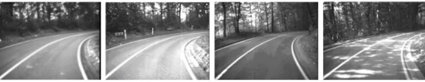
In this work, a sequence of gray-level images will be analyzed, via on-board single camera, in order to describe the road shape . On vision-based intelligent vehicles, different approaches [2, 7] have been proposed to deal with complex situations such as intersections and junctions. Using a single camera as sensor, a transform as filter, and a non-supervised neural network as classifier, we want to create a simple and fast solution, which is robust for noise, discontinuity, contrast variation, and shadows (Figure 1). The system should be capable of detecting and classifying road singularities, such as shape, relative curve orientation, presence of intersections, etc. A dynamic process may then guide the analysis of the following images in the sequence.

Figure 1: Different image configurations on the same road situation. The following section describes the implemented method: the Hough Trans-form, used to detect the road shape, and the Self-organizing Map (SOM), used

as classification method. Section 3 gives a quality index for evaluating the training results and its applications on some simulations. The last section presents conclusions and proposals for future work.

2

Method

In a system that characterizes objects present in an image, we must first estab-lish a representation that may better describe the information. Previous studies in the literature show that object recognition is improved when it uses the ob-ject contours instead of the absolute luminance values (gray levels) [1, 6, 9]. This representation is more robust for luminance intensity and to direction changes.

2.1

Feature extraction

Feature extraction can be seen as a special kind of data reduction for which the goal is to find a subset of informative variables based on image data. Since image data is, by nature, very high dimensional, feature extraction is often a necessary step for objet recognition to be successful. It is also a means for controlling the so–called curse–of–dimensionality. When used as further inputs, one wants to extract those features that best describe the objects in the image, preserving the class separability.

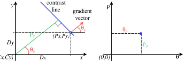
Intuitively, road contours may be simplified as a set of curves. Recent works have tried to describe these curves as polynomial equations, splines, etc. [10, 11]. The Hough Transform [5] is a well known technique for detecting para-metric lines, curves and other shapes. In this work, the transform establishes a link between the line (or line segments) of an image from a Cartesian represen-tation to a polar represenrepresen-tation using as parameters: the angle θ ∈ [−180, 180] perpendicular to the contrast line (its gradient vector) and the distance ρ from this line to the center point (Cx, Cy). Unlike the classical Hough Transform calculus, we do not analyze several possible angles and distances, but simply calculate the local gradient [3], as detailed below.

(Cx,Cy) contrast line Dx Dy ρ θ x y (0,0) ρ θ (Px,Py) gradient vector P ρ P P θP θ_P

Figure 2: Principle of the Hough Transform. Given a pixel P and its contrast line, the distance between this line and a center point C is calculated using the gradient angle θ.

Suppose that the pixel (Px, Py) can be represented by a function of the luminance intensity I(x, y). The gradient vector is calculated from the vertical

and horizontal luminance variations between the neighboring pixels: Gvertical=

I(x − 1, y) − I(x + 1, y) and Ghorizontal= I(x, y − 1) − I(x, y + 1), respectively, i.e.:

θ = tan−1³ Gvertical Ghorizontal

´

(1) Let Dx= Px−Cxand Dy = Py−Cy, as illustrated in Figure 2, the distance

ρ from the defined contrast line (perpendicular to the gradient) to the center

point can be calculated as:

ρ = Dx∗ cos θ + Dy∗ sin θ (2) Hence, Equations (1) and (2) define a mapping (x, y) ∈ <2_{to (θ, ρ) ∈ <}2_.

From the definition, each line (even when discontinuous in the image) be-comes a point on the new representation. If the curves can be approximated by a set of line segments, then it will be transformed into a cloud of points in the new representation. In particular, intersection curves in the scene will be represented as separated clouds of points.

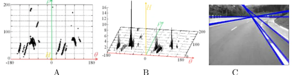
The result of the feature extraction is a histogram describing the relevant contrast lines on the scene (see Figure 3–A and B). The inverse transformation of the highest points on the histogram gives the main lines of the road curves (Figure 3–C).

A B C

Figure 3: From a gray level image of a turn to the right, the 3D histogram of the θ, ρ Hough Transform was extracted (A and B). The inverse transformation is applied on the histogram maxima, recreating lines on the Euclidean space.

Given that a line is described on the Euclidean space by the equation y =

ax + b and that the calculations of θ and ρ may be described as functions of a

and b, the Hough Transform may be formalized by a pair of functions: h a b i H −→ h θ ρ i

where θ = f (a, b)_{ρ = g(a, b)}

The Jacobian determinant of the above functions shows that the best way to give weight to the entries is proportional to the gradient vector norm. In this case, the vectors with small norm, the ones more sensitive to noise, have a smaller contribution on the histogram. Besides, null gradient vectors (uniform regions) are automatically eliminated, as shown in the histograms at Figure 4.

Figure 4: The 2D histogram was calculated for the θ gradient angles on original image. The full-line shows the noise accumulated on the histogram when adding 1 for each θ instance found on the image, and the clear peaks on the dot-line curve when the entry is proportional to the norm of the corresponding the gradient angle.

2.2

Classification

A wide class of artificial neural networks can be trained to perform classifica-tion. In this paper, we apply a SOM [8] to organize structural road changes in topological manner. The structural information obtained by the previ-ous feature extraction step is collected in a d dimensional vector x (where

d = M AXθ∗ M AXρ, the dimensions of the 3D histogram). These vectors are quantized into a finite number of so–called centroids using a SOM that offers several advantages such as the ability to quantize adaptively depending on the ranges of the attributes and the ability to deal with the curse–of–dimensionality. The network has one layer of n units arranged in a grid. The set I = 1, ..., n of units is composed in a topological structure. This is provided by a symmetrical and decreasing neighborhood function Λ(i, j), defined on I x I. The input space X is included in <d_{. The units are fully connected to the} inputs, and xij represents the strength of connection between unit i and the

jth_{component of the input. The unit i is defined by the vector:}

wi= (wi1, wi2, ..., wid) (3) For a given state S, the network response to input x is the winner unit io, the closest unit to input x. Thus, the network defines a map ΦS: x 7−→ i(x, S), from w to I = 1, ..., n, and the goal of the learning algorithm is to converge to a network state such that the corresponding map will be topology preserving. The learning step is formalized as in Equation (4), where ε is the decreasing learning rate.

wi(t + 1) = wi(t) − ε(t)Λ(io, i)(x(t) − wi(t)) (4) Using N as the number of iterations, we applied the following Gaussian function as a linear decreasing Λ(io, i)

Λ(io, i) = e ¡ −||io−i||2 2σ(t) ¢ where σ(t) = 1 + (σ(0) − 1) ∗³ 1 − t N ´ (5)

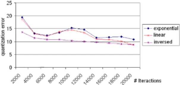
There are no known proof to the SOM training convergence, but some statistical measures can be made to evaluate the quality of the map [4]. To improve the SOM convergence, we studied the mean quantization error dur-ing the traindur-ing with 3 learndur-ing rate decreasdur-ing functions: linear, exponential and inversed proportional to time (see Figure 5). Given β an initialization parameter, Equation (6) shows the used function.

Figure 5: The error evolution (the square distance of an input xi and its winner

centroid) showed that the best performance is with the inversed decreasing function described bellow. ε(t) = ε(0) ∗ Ã ¡_N β ¢ ¡_N β ¢ + t ! (6)

3

Simulations

1173 gray scale images, with 384*288 pixels, were taken from a camera installed on the roof of the experiment car. Several lighting conditions were encountered, depending on the position of the sun and on the shadows provided by trees and various objects. From the continuous recording, we manually selected a proportionally distributed training set of 978 representative images.

The described methodology was applied to each image, and their collected histograms were used as input to the neural network. These histograms were downsampled with a scale of 10, creating input vectors of d = (36 ∗ 20) = 720. 5 manual labels were established giving a class to each test image: turn to the

right, turn to the left, straigh road, side road junction and roud-about. As a

supervised step, the test set was presented and centroids class were defined by the label classified more often. The final result of the simulation shows the number images of the labels that were recognized on the same class label:

Test-set size Right results Recognition rate

right turn 93 79 84.9%

straigt road 444 331 74.5%

left turn 57 51 89.5%

4

Conclusion and Future Work

In this paper, we develop a solution for detecting and classifying road singular-ities. The scene geometry is described by a set of lines, extracted by a Hough transform. These parameters are treated by a SOM network.

The chosen side road junction images sequences were always in straight road situations. Besides, the lack of contrast and absence of road marks on most of the intersection roads images opened the way to the confusion between the 2 classes. A better set of images should be included on the training set to improve the separability of the classes. The round-about sequences represented all the 4 steps of the round-about: approaching, driving in, turning around and driving out. These complex situations create some other confusions. The round-about should be splited in different classes (for example, the turning around seems close to the turn to the left).

Although we present a simple supervised output for the SOM clusters, we have chosen the Kohonen map to be able to analyze the behaviour of the sequence classification on the neighborhood topology, in a following step.

Initial results with a light/dark band detector show some interesting im-provements on the detection the intersection and on the reduction of noise (shadows, textures, etc.). This should be better studied to try to ameliorate the feature extraction.

References

[1] R. Brunelli and T. Poggio. Face recognition: Features versus templates. IEEE

Trans. on Pattern Analysis and Machine Intelligence, 15(10):1042–1052, 1993.

[2] J.D. Crisman and C.E. Thorpe. Scarf - a color vision system that tracks roads and intersections. IEEE Trans. on Robotics and Automation, 9(1):49–58, 1993. [3] R. Cucchiara and F. Filicori. The vector-gradient hough transform. IEEE Trans.

on Pattern Analysis and Machine Intelligence, 20(7):746–750, 1998.

[4] E. de Bold, M. Cotrell, and M. Verleysen. Statistical tools to asses the reliability of self-organizing maps. Neural Networks, 15:967–978, 2002.

[5] R.O. Duda and P.E. Hart. Use of the hough transform to detect lines and curves in pictures. Communications of the ACM, 15:11–15, 1972.

[6] S. Edelman, N. Intrator, and T. Poggio. Complex cells and object recognition. submitted, 1997.

[7] T.M. Jochem, D.A. Pomerleau, and C.E. Thorpe. Initial results in vision based road and intersection detection and traversal. Technical Report CMU-RI-TR-95-21, The Robotics Institute, Carnegie Mellon University, 1995.

[8] T. Kohonen. Self-organizing maps. Springer, Berlin, 1995. [9] D. Marr. Vision. Freeman and Company, New York, 1982.

[10] J.-P. Tarel and F. Guichard. Combined dynamic tracking and recognition of curves with application to road detection. Proc. IEEE ICIP, September 2000. [11] Y. Wang, D. Shen, and E.K. Teoh. Lane detection using catmull-rom spline.