1
Simulation of a Two-Slope Pyramid Made by SPIF using an
Adaptive Remeshing Method with Solid-Shell Finite element
J. I.V. de Sena
a,b, C. F. Guzmán
b, L. Duchêne
b, A. M. Habraken
b, A.K. Behera
c,
J. Duflou
c, R. A. F. Valente
a, R. J. Alves de Sousa
aaGRIDS Research Group, TEMA Research Unity, Department of Mechanical Engineering, University of Aveiro,
3810 Aveiro, Portugal, [email protected], [email protected], [email protected]
bUniversité de Liège, ArGEnCo Department, MS²Fdivision, Chemin des Chevreuils 1, Liège, 4000, Belgium,
[email protected], [email protected], [email protected]
cKatholieke Universiteit Leuven, Department of Mechanical Engineering, Celestijnenlaan 300B, B-3001 Leuven,
Belgium, [email protected], [email protected]
Abstract
Single point incremental forming (SPIF) is an emerging application in sheet metal prototyping and small batch production, which enables dieless production of sheet metal parts. This research area has grown in the last years, both experimentally and numerically. However, numerical investigations into SPIF process need further improvement to predict the formed shape correctly and faster than current approaches.
The current work aims the use of an adaptive remeshing technique, originally developed for shell and later extended to 3D “brick” elements, leading to a Reduced Enhanced Solid-Shell formulation. The CPU time reduction is a demanded request to perform the numerical simulations. A two-slope pyramid shape is used to carry out the numerical simulation and modelling. Its geometric difficulty on the numerical shape prediction and the through thickness stress behaviour are the main analysis targets in the present work. This work confirmed a significant CPU time reduction and an acceptable shape prediction accuracy using an adaptive remeshing method combined with the selected solid-shell element. The stress distribution in thickness direction revealed the occurrence of bending/unbending plus stretching and plastic deformation in regions far from the local deformation in the tool vicinity.
Keywords: Adaptive remeshing; Solid shell finite element; Single point incremental forming.
1. INTRODUCTION
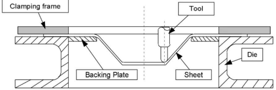
The research interest in Incremental Sheet Forming (ISF) processes has been growing in the last years, both experimentally and numerically, in the context of sheet metal forming processes. The designation of incremental forming processes covers several techniques with common features. A review on technical developments of ISF variants in the last years can be found in the work of Emmens et al. (2010). In the present work, particular attention will be dedicated to the Single Point Incremental Forming (SPIF) variant as shown in Figure 1.
2
SPIF process reveals itself as an interesting application due to its flexibility, where symmetrical or asymmetrical shapes can be built. This process flexibility is given by the motion of a single spherical tool without any type of die or mould needed. This means that the sheet side opposite to the tool does not contact with any mould or support. The dieless nature of SPIF process was first envisioned by Leszak (1967). The use of this method was possible with the advance of technology, more specifically with the appearance of numerical control machines. The tool path can be controlled by using CAD/CAM software, where a change in the final shape can be quickly and inexpensively done. The pre-programmed contour combines continuous contact of the tool along the sheet surface with successive small vertical increments. After each vertical increment, a contour in the next horizontal plane starts, with the final component being constructed layer by layer. The sheet is previously clamped along its edges using a clamping frame (blank holder). A backing plate can be needed with the objective to decrease springback effect during the forming progress. Springback phenomena can also be avoided using a compensatory algorithm (Allwood et al., 2010).
Due to the vast number of new topics to explore, many works have been carried out. A number of authors have experimentally and numerically studied the final product geometry in order to analyse the influence of several parameters involved in the SPIF process. From the numerical standpoint, force prediction and geometric inaccuracy on SPIF simulation can be provided by Finite Element Method (FEM). In previous academic research works, Rabahallah et al. (2010) and Guzmán et al. (2012) the force prediction and shape prediction were studied. In both works a special focus was given to a two-slope pyramid which is a challenge in terms of computation time and prediction of force and shape accuracy. Both authors have used a shell finite element in their FEM analysis. However, Duchêne et al. (2013) have used a solid-shell finite element in order to investigate the influence of Enhanced Assumed Strain (EAS) formulation in the accuracy of the shape.
The numerical simulations consist in the use of an adaptive remeshing as strategy to reduce the CPU time. The numerical shape prediction is compared with experimental measurements along the middle section of the sheet. The selection of three finite elements on distinct regions of the sheet mesh along the middle section is used to analyse the stress behaviour in thickness direction. The analysis of the stress components can allow the understanding of the main deformation mechanisms responsible for the formability within SPIF process.
2. NUMERICAL SIMULATIONS
The numerical simulations include an adaptive remeshing algorithm combined with a hexahedral finite element, which is a solid-shell finite element. It is worth noting that no previous work has been carried out using remeshing strategies with solid elements for SPIF, which makes this work innovative.
2.1. Adaptive remeshing technique
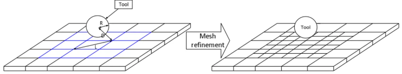
The adaptive remeshing method was implemented within an in-house implicit FEM code called LAGAMINE, developed at the University of Liège (Lequesne et al., 2008) and initially applied to a shell element COQJ4 finite element (Jetteur and Cescotto, 1991; Li, 1995). In the present work, this technique was extended to be used with solid-shell finite element, with a RESS formulation (Alves de Sousa et al, 2005, 2006, 2007). The main principle of this numerical technique is based on the fact that only a portion of the blank mesh is dynamically refined in the tool vicinity, following its motion. Doing so, the requirement of initially refined meshes can be avoided and consequently, the global CPU time can be reduced (Figure 2).
3
The adopted remeshing criterion is based on the shortest distance between the centre of the spherical tool and the nodes of the finite element. The size of the tool vicinity is defined by the user through the expression:
2 2 2
D
α(L + R ) ,
(1) where D is the shortest distance between the center of the spherical tool and the nodes of the element, L is the longest diagonal of the element, R is the radius of the tool and α is a neighborhood coefficient also chosen by the user.Following this idea, the coarse elements respecting the criterion (eq. 1) are deactivated and become a “refined cell” which contains all information about new smaller elements. Each coarse element is divided into a fixed number of new smaller elements. The partition of each coarse mesh is based on the number of nodes division per edge (n) defined by the user. The transference of stress and state variables from the coarse element to the new elements is performed by an interpolation method. This interpolation method is based on a weighted-average formula from the work of Habraken, (1989). If the tool is farther from a refined element and the “cell” does not respect the criterion (eq.1), the new elements are removed and the coarse element is reactivated. However, the shape prediction could be less accurate if the new elements are removed. Consequently, an additional criterion is used to avoid losing accuracy. If the distortion is significant, the refinement remains on the location of the coarse element. This is based on the distance, d, between the current position of every new node, Xc, and a virtual position, Xv. The
virtual position is the position of the new node when it has the same relative position in the plane described by the coarse element, as illustrated in Figure 3.
Figure 3: Distortion criterion, lateral view. The criterion for reactivating a coarse element is given by:
where
max c v
d
d
d =
X
-
X
.
(2)where dmax is the maximum distance chosen by the user.
As this refinement method does not take into account any transition zone between coarse and refined elements, there are three types of nodes: old nodes, free new nodes and constrained new nodes. The constrained nodes are used to allow the structural compatibility of the mesh. The degree of freedom (DOF) and positions of the constrained nodes on a “cell” edge depend on the two old nodes (masters), which are extremities of this edge. The variable number of DOF induces a modification in the equilibrium force and in the stiffness matrix. During the SPIF process simulation many elements are refined and coarsened, so as a result many cells are created and removed. A “linked list” is used as a data structure to insert and remove cells at any point in the list. More details of this adaptive remeshing technique can be found in the work of Lequesne et al. (2008).
2.2. Finite element formulation
The RESS finite element is a hexahedral element composed by 8 nodes and each node has three DOF. A combination of Enhanced Assumed Strain method (EAS) (Simo and Rifai, 1990) and hourglass stabilization in the element reference plane, with the use of an arbitrary number of integration points in thickness direction, characterize this formulation. The volumetric locking effect is reduced using the EAS method and the reduced integration in the element plane. These choices give more deformation modes to the finite element structure. However, the reduced integration in the element plane provides spurious modes of deformation called hourglass phenomena. Consequently, the mentioned stabilization scheme is used to alleviate the hourglass effect. More detailed information of this formulation can be found in the series of works of Alves de Sousa et al. (2005, 2006 and 2007).
The use of a conventional solid element requires several element layers to correctly capture bending effects and multiple layers of finite elements along the thickness increases the computation time. Figure 4 schematically presents the advantage of RESS finite element structure compared with different 3D finite elements scheme available in some commercial softwares.
4
a) b) c)
Figure 4: Comparison between fully integrated (a), reduced integrated (b) and RESS finite elements (c).
The choice of a solid-shell formulation to simulate sheet metal forming operations is also based on the possibility to use a general 3D constitutive law of material behavior, while classical shell finite elements are implicitly based on plane stress/strain assumptions. Additionally, thickness variations and double-sided contact conditions are easily and automatically considered with solid-shell finite elements.
3. TWO-SLOPE PYRAMID NUMERICAL VALIDATION
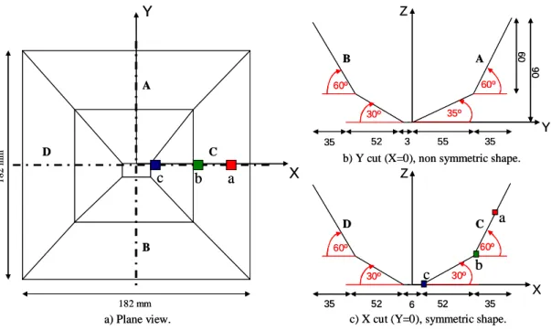
The numerical simulation of SPIF addressed in the current section consists of a two-slope pyramid benchmark with two different depths. The sheet material is low carbon steel alloy, DC01, with an initial thickness of 1.0 mm, being clamped on its border by means of a 182 mm x 182 mm blank holder. The tool tip diameter is 10 mm and the tool path is based on successive quadrangular paths with a vertical step size of 1.0 mm per contour. The number of contours for the first slope of the pyramid is 60 and 30 contours are present in the second slope. The experimental tool path points were given in order to use it in the numerical simulations. These SPIF experiments as well as the shape measurements were performed by the team at KU Leuven (Duchêne et al., 2013) who provided all the required data for the numerical simulations and their validation. The dimensions of an ideal design are schematically shown in Figure 5.
Y
X
182 mm 1 8 2 m m A B C D a) Plane view.a
b
c
Y
X
182 mm 1 8 2 m m A B C D a) Plane view.a
b
c
Y Z Z X 35 52 6 52 35 35 52 3 55 35 6 0 9 0 30º 30º 60º 60º 30º 35º 60º 60ºb) Y cut (X=0), non symmetric shape.
c) X cut (Y=0), symmetric shape. A B C D
a
b
c
Y Z Z X 35 52 6 52 35 35 52 3 55 35 6 0 9 0 30º 30º 60º 60º 30º 35º 60º 60ºb) Y cut (X=0), non symmetric shape.
c) X cut (Y=0), symmetric shape. A B C D
a
b
c
Figure 5 - Component nominal dimensions.
The shape analysis is divided in four sections (A, B, C, D), in order to analyse them separately in the middle section of the mesh model (see Figure 6), to avoid the influence of Boundary Conditions (BC). The material behaviour is elastically described by E = 142800 MPa and ν = 0.33. The hardening type adopted is a mixed one, with an isotropic constitutive model. The kinematic part of the hardening is introduced by a back-stress tensor described by non-linear Armstrong-Fredrick model (Duchêne et al., 2013). The plastic domain is described by a von
5
Mises yield surface and the isotropic hardening behaviour is defined by means of a Swift’s law. The chosen parameters are listed on Table 1. The initial yield stress (σ0 ) is 144.916 MPa.
Table 1 – Material parameters.
Name and hardening type Swift parameters Back-stress
Swift
Isotropic hardening K=472.19MPa; n=0.171; ε0=0.001 Cx=51.65; Xsat=5.3
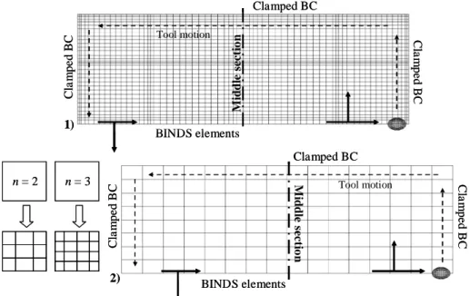
Figure 6 illustrates two distinct meshes refinements. Due to the square geometry in XY plane (see Figure 5.a) and to benefit the computation time reduction, only half of the sheet is modelled. This simplification also can provide a similar result as a full mesh (Henrard, 2008). The initial refined mesh (reference mesh) is composed by 2048 elements disposed in one layer of RESS finite element in thickness direction. The coarse mesh used with adaptive remeshing method is modelled by 128 elements on the sheet plane with one layer of RESS finite element in thickness direction. However, the nodes at the top layer of both meshes define the contact element layer at the surface. The contact modelling is based on a penalty approach and on a Coulomb law (Habraken and Cescotto, 1998). So, both meshes have two layers of elements (solid-shell + contact element) in thickness direction, and the spherical tool was modelled as a rigid body. Finally, Coulomb friction coefficient between the tool and sheet is set to 0.05 (Henrard et al., 2010) and the penalty coefficient is equal to 1000 [N.mm-3].
Clamped BC C la m p e d B C C la m p e d B C C la m p e d B C Cla m p e d B C Clamped BC BINDS elements BINDS elements M id d le s e c tio n M id d le s e c ti o n n = 3 n = 2 1) 2) Tool motion Tool motion Clamped BC C la m p e d B C C la m p e d B C C la m p e d B C Cla m p e d B C Clamped BC BINDS elements BINDS elements M id d le s e c tio n M id d le s e c ti o n n = 3 n = 2 1) 2) Tool motion Tool motion
Figure 6 - Reference mesh (1) and coarse mesh used with adaptive remeshing (2).
The numerical shape prediction is extracted from the middle section of the half mesh used within the FE model. To avoid inaccuracy due to BC effect, each pyramid wall section is analysed separately.
Displacement BC was imposed (see Figure 6) in order to minimize the effect of missing material at both central edges along the symmetric axis. This type of BC is introduced by a finite element called BINDS and it is a link between the node displacements of both edges (Bouffioux et al., 2010; Henrard et al., 2010). The absence of backing plate and blank holder in the numerical model was replaced by the clamped BC at the borders of both meshes. The absence of clamping devices avoids more contact interactions during the numerical computation, beyond the tool contact motion, decreasing CPU time.
Different values for each parameter were tested for derefinement distance (dmax) as well for the number of
nodes per edge (n): dmax values were 0.1 mm and 0.2 mm; n values were 2 and 3 nodes. The value used for α
coefficient is equal to 1.0. These values used for each remeshing parameter were chosen based on a previous sensitivity analysis using the line-test benchmark simulation (Bouffioux et al., 2008). The total number of elements
6
in both meshes includes the number of all finite elements of the model (RESS+CFI3D+BINDS). The number of integration points through the thickness used in RESS finite element is 5 Gauss Points (GP).
Table 2 presents the adaptive remeshing procedure performance. It is possible to confirm the adaptive remeshing advantages even when the final number of elements is higher than the reference mesh.
Table 2 – Adaptive remeshing technique performance.
Mesh type CPU time CPU time
Reduction (%) Initial nº of elements Final nº of elements
n=2 dmax=0.1mm 6h:28m:25s 76.67 298 2602 n=3 dmax=0.1mm 13h:38m:43s 50.8 4394 dmax=0.2mm 13h:18m:2s 52.1 4394 Reference 27h:44m:27s --- 4282 4282
The application of the adaptive remeshing with n equal to 3 allows a CPU time reduction of 50% when negligible difference for different values of dmax parameter is observed. The CPU time reduction using n equal to 2
is considerably larger than for n equal to 3. However the accuracy obtained with different refinement levels are analysed in the following section.
The main numerical outputs presented in the next sections are the final shape of the sheet, in a middle-section along the symmetric axis in different directions (see figures 5.b and 5.c) and stress state behaviour. The deformed shape evolution is also analysed for different tool depths.
3.1. Shape prediction
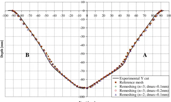
In the current section, the deformed shape predictions from the bottom nodes are compared to the available experimental results. The experimental shape measurements were extracted using Digital Image Correlation (DIC) throughout the SPIF process (Guzmán et al., 2012). Figure 7 exhibits the shape prediction in Y direction using the adaptive remeshing procedure in simultaneous comparison with the reference mesh and experimental measurements. Different adaptive remeshing parameters are tested in order to assess their influence in the numerical shape accuracy. -100 -90 -80 -70 -60 -50 -40 -30 -20 -10 0 10 -100 -90 -80 -70 -60 -50 -40 -30 -20 -10 0 10 20 30 40 50 60 70 80 90 100 Y cut [mm] D e p th [ m m ] Experimental Y cut Reference mesh Remeshing (n=3; dmax=0.1mm) Remeshing (n=3; dmax=0.2mm) Remeshing (n=2; dmax=0.1mm)
Figure 7 - Final shape prediction in Y cut for different refinement levels after the tool unload.
7
It can be observed in Figure 7 that an acceptable accuracy is achieved between the numerical results and the experimental measurements. The derefinement criterion occurs with more frequency using dmax equal to 0.2 mm
than for dmax equal to 0.1 mm. A low value of dmax parameter means that the refinement is kept increasing the mesh
flexibility. In this case, at the transition region of wall-angle on section A, the adaptive remeshing using n equal to 3 combined with dmax equal to 0.2 mm seems more accurate than the others numerical simulations results. Figure 8
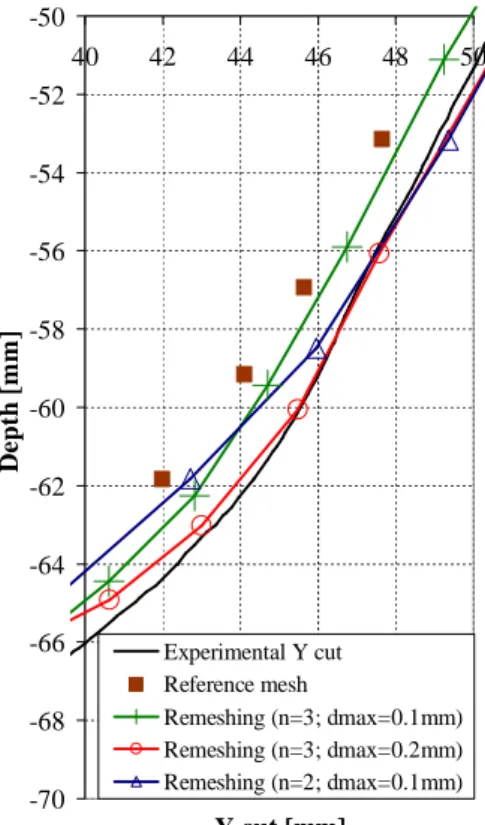
exhibits a zoom at wall-angle change of section A, which evidence a better shape prediction using n equal to 3 combined with dmax equal to 0.2 mm.
-70 -68 -66 -64 -62 -60 -58 -56 -54 -52 -50 40 42 44 46 48 50 Y cut [mm] D e p th [ m m ] Experimental Y cut Reference mesh Remeshing (n=3; dmax=0.1mm) Remeshing (n=3; dmax=0.2mm) Remeshing (n=2; dmax=0.1mm)
Figure 8 – Zoom of shape prediction at wall-angle change on section A in Y cut for different refinement levels. In the following, the average relative and absolute errors are computed and presented in Table 3 for each refinement level. The difference between the numerical result along the middle section on the meshes and the experimental measurements is computed for the common values in the corresponding axis. Previously, the numerical values along of middle cross section were linearly interpolated for the corresponding values of experimental measurements. The average relative error is computed using the following expression:
N 2 2 i=1 (Num. - Exp.) Error(%) = N * 100 Exp.
(3)where Num. is the numerical value, Exp. is the experimental value and N is the number of points in X axis. Table 3 – Average error for Y cut section A.
Y cut (A) Remeshing mesh Reference mesh
Error Relative (%)
n=3; dmax =0.1mm 5.95
6,37
n=3; dmax =0.2mm 5.32
8
In general, the refinement level using adaptive remeshing method with n equal to 3 nodes per edge presents better approximation to the experimental results than the reference mesh and n equal to 2 nodes per edge. However, an improvement was obtained using n equal to 3 combined with dmax equal to 0.2 mm at the wall-angle transition
region. Its absolute error at wall-angle change is equal to 0.12 mm while using n equal to 3 and dmax equal to 0.1 mm
the absolute error at wall-angle change is 2 mm.
The section B of Y cut presents a similar behavior as the section A, as can be seen in Table 4). However, the absolute error at the wall-angle change is more noticeable on section B for n equal to 3 nodes per edge with different values of dmax. It presents an absolute error of 3.53 mm using dmax equal to 0.1 mm and the error decrease to
2.49 mm using dmax equal to 0.2 mm.
Table 4 – Average error for Y cut section B.
Y cut (B) Remeshing mesh Reference mesh
Error Relative (%)
n=3; dmax =0.1mm 6.63
6.94
n=3; dmax =0.2mm 6.37
n=2; dmax =0.1mm 9.93
In this first cut analysis, the section A has better shape accuracy than the cut B. However, for both sections a better shape accuracy was achieved using a dmax value equal to 0.2 mm. Probably, this fact occurred due to a
derefinement at some regions of the wall angle mesh during the simulation forming, which leads to an improvement at the wall-angles transition area.
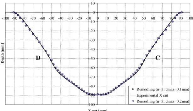
Figure 9 exhibits the shape predictions in X direction using the adaptive remeshing procedure after tool unload. The numerical result below was obtained using the adaptive remeshing parameters n equal to 3 nodes per edge with different dmax values of 0.1 mm and 0.2 mm.
-100 -90 -80 -70 -60 -50 -40 -30 -20 -10 0 10 -100 -90 -80 -70 -60 -50 -40 -30 -20 -10 0 10 20 30 40 50 60 70 80 90 100 X cut [mm] D e p th [ m m ] Remeshing (n=3; dmax=0.1mm) Experimental X cut Remeshing (n=3; dmax=0.2mm)
Figure 9 - Final shape prediction in X cut for refinement n equal to 3 nodes per edge, after tool unload.
The numerical results on the X cut are considered symmetric, once the wall-angles of sections C and D are similar. Table 5 presents the average error in X direction, at the middle section.
C
D
9
Table 5 – Average error for Y cut section C or D.
X cut (C and D) Remeshing mesh
Error Relative (%)
n=3; dmax =0.1mm 4.72
n=3; dmax =0.2mm 4.77
The average relative error analysis of X cut using dmax equal to 0.1 mm is negligibly smaller than the use of
dmax equal to 0.2 mm. However, at transition region of wall-angle change, and it is visible that for dmax equal to 0.1
mm the shape accuracy is better than for dmax equal to 0.2 mm.
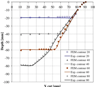
Figure 10 exhibits the comparison between the experimental measurements and the numerical results of four different contours. The numerical curves are intentionally shifted to coincide with experimental at similar depth value. The missing data of the experimental measurements near the backing plate and near of X equal to 0 mm are difficult to extract with the use of DIC (Guzmán et al., 2012). The numerical results were obtained using the adaptive remeshing method with n equal to 3 nodes per edge and dmax equal to 0.1 mm.
-100 -90 -80 -70 -60 -50 -40 -30 -20 -10 0 0 10 20 30 40 50 60 70 80 90 100 X cut [mm] D e p th [ m m ] FEM contour 20 Exp. contour 20 FEM contour 40 Exp. contour 40 FEM contour 60 Exp. contour 60 FEM contour 80 Exp. contour 80
Figure 10 - Shape prediction for X cut at different depth steps using the adaptive remeshing method.
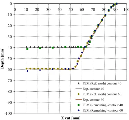
The numerical results follow the overall shape of the experimental measurements for the contours 20 mm to 60 mm. However, there is a difference at the central region of the mesh due to non-refined area of contours 40 mm and 60 mm. This difference occurs when the refinement and derefinement criteria were not achieved in the finite elements near the central area of the mesh. Firstly, due to distance between the tool and the nodes in the tool vicinity (see Figure 12.1) and secondly, due to no significant deformation happening in mesh plane (see Figure 3). To understand the deviation occurrence at the central region of the mesh for contours 40 mm and 60 mm using the adaptive remeshing method, a new analysis was carried out. Thanks to a simulation using the reference mesh of Figure 6.1 and another one with adaptive remeshing method and a new value of α coefficient equal to 3 combined with dmax equal to 0.1 mm, accuracy at the central area of the meshes has been further analysed. Figure 11 presents
10 -100 -90 -80 -70 -60 -50 -40 -30 -20 -10 0 0 10 20 30 40 50 60 70 80 90 100 X cut [mm] D ep th [ m m ]
FEM (Ref. mesh) contour 40 Exp. contour 40
FEM (Ref. mesh) contour 60 Exp. contour 60
FEM (Remeshing) contour 40 FEM (Remeshing) contour 60
Figure 11 - Shape prediction for X cut at 40 mm and 60 mm of depth.
The obtained results using the reference mesh proves that the refinement at the central region avoids the numerical deviation error. However, even with a high value of α coefficient the deviation using the adaptive remeshing the deviation continues, due to fulfil the derefinement criterion. The refinement at the central area remains if a significant distortion occurs and if the dmax value is higher than the value chosen by the user. Once the
forming tool does not move on the referred region, the refinement due to a high value of α coefficient is deleted and the coarse elements are reactivated.
At 80 mm depth, Figure 10 presents a visible error in the transition zone of the wall-angle. This shape error was mentioned by Guzmán et al. (2012) (see Figure 12 in Guzmán et al., 2012) as the “tent” effect. In order to understand the origin of this shape inaccuracy after wall-angle transition, the following section will present a stress analysis in the thickness direction.
3.2. Through thickness stress
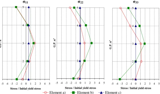
The main interest of the current section is the analysis of stress state in thickness direction in different wall regions of the mesh at the middle section. The stress state is obtained using the adaptive remeshing technique at the end of two different forming stages. Figure 12 exhibits the mesh plane view and the elements selected.
1)
σ
11
σ
2211 2)
Element a) Element b) Element c)
Figure 12 –Position of three selected elements after contour 60 mm (1) and after contour 90 mm unloading step (2). The stress analysis behaviour of each Gauss Point (GP) through thickness is performed at different forming depths for three selected elements. The GP positions are such that GP1 is near the sheet external surface (the one not in contact with the tool) and GP5 near the internal surface. The orientation of the local stresscomponents in plane are σ11 andσ22 can be recovered by their projections in Figure 12. The component σ33 is the stress state in thickness direction.
Figure 13 presents the relative stress (σ/σ0) values (σ0 being the initial yield stress 144.916 MPa) at the 60th contour (at the beginning of the forming of the second slope pyramid when the tool has already had contact with the sheet and going deeper). The associated mesh and the tool position is shown in Figure 12.1.
σ
11σ
22σ
33 1 2 3 4 5 -5 -4 -3 -2 -1 0 1 2 3 4 5Stress / Initial yield stress
G .P . n º 1 2 3 4 5 -5 -4 -3 -2 -1 0 1 2 3 4 5
Stress / Initial yield stress
G .P . n º 1 2 3 4 5 -5 -4 -3 -2 -1 0 1 2 3 4 5
Stress / Initial yield stress
G
.P
.
n
º
Element a) Element b) Element c)
Figure 13 – Stress components through the thickness for the three elements at depth stage 60 mm.
The cyclic strain path associated to SPIF, checked by He et al. (2006), confirms the bending/unbending type of load associated to a stretch forming. The σ11 andσ22 stress components (Figure 13) of the element a) at middle position on the 60º wall has a typical scheme resulting from such stress state. Guzmán et al. (2012) used a shell finite element to analyse a two slope pyramid made in Aluminum AA3003, similar to the DC01 pyramid studied in the present work. As expected, the stress states computed by shell and solid-shell approaches present both similarities and discrepancies. The results from Guzmán et al. 2012 were based on the shallow shell theory, thus they assumed that the mid-plane coincides with the neutral plane. The solid-shell element formulation allows a
σ
11σ
2212
greater flexibility and takes into account through thickness shear stresses and normal stress in thickness direction in addition to the membrane stresses. The deformation characteristics of SPIF during the tool contact could induce a strong element deflection (as probed by the choice of dmax equal to 0.2 mm in the previous section). Hence, the shell
hypothesis of the mid/neutral plane could be considered as somewhat severe. The membrane stress distribution in Figure 13 for element (a) and (b) could be considered as the sum of bending/unbending plus stretching, as previously observed by Eyckens et al. 2010. The typical stress distribution is depicted schematically in Figure 14 assuming for simplicity elastic behaviour. Indeed true behaviour is more complex as plasticity occurs in both bending and unbending processes (see equivalent plastic strain values in Table 6) and local contact generating σ33 as well as through thickness shear stresses justifies a slightly higher plastic strain near internal surface. The stress profile of σ33 related to element a) in the wall middle section presents the typical gradient expected due to tool contact. The GP near the internal surface (GP 5) is associated to the tool compression effect during the forming path and zero stress on the external surface (GP 1). For element b) at change of slope, a more complex pattern of σ33 is observed due to further plasticity increase at this location during the forming of the second pyramid, however higher number of GP computation confirms a null stress at external surface.
=
+
+
1 2 3 4 Neutral plane Δm=
+
+
1 2 3 4 Neutral plane ΔmFigure 14 – Simple elastic schematic representation of bending/unbending plus stretching associated to elements a) and b).
Figure 15 presents the relative stress (σ/σ0) values at 90 mm depth for each GP through the sheet thickness. Figure 12.2 is its corresponding mesh, note that the tool has been removed, it is an unloaded configuration.
σ
11σ
22σ
33 1 2 3 4 5 -5 -4 -3 -2 -1 0 1 2 3 4 5 Stress /Initial yield stressG .P . n º 1 2 3 4 5 -5 -4 -3 -2 -1 0 1 2 3 4 5 Stress /Initial yield stress
G .P . n º 1 2 3 4 5 -5 -4 -3 -2 -1 0 1 2 3 4 5 Stress/Initial yield stress
G
.P
.
n
º
Element a) Element b) Element c)
13
The elements a) and b) at the end of contour 90 have a similar stress profile to the pattern of contour 60, however, they present identical or higher values stress values. The strong increase of membrane stresses of GP 5 compared to Figure 13 as well as the values of equivalent plastic strain in Table 6 confirm that additional plastic deformation appeared at depth 60 (change of pyramid slope) during further forming (increased value from 0.599 to 0.855). Already mentioned in the work of Guzmán et al. (2012), the “tent” effect (Behera et al. 2011, 2012, 2013, 2014) called from displacement of the material at depth 60 mm during second pyramid forming (see Figure 11) happens. As explained in Figure 12 of Guzmán et al. (2012), structural bending effect far from the tool location induces this displacement as the smaller slope angle increases the lever arm of the tool force and generates high moment in this transition zone. Guzmán et al. 2012 showed that it occurs only as an elastic effect for their case, however in the present work a different material is used and plastic strain in element b) clearly increases between contour at 60 and 90mm depth. Comparing element b) at contour depth 60mm (Figure 13) and element c) at contour depth 90mm in Figure 15 and in Table 6, one can observed typical differences of stress states in SPIF formed shapes with high and low slopes respectively. Plastic strain levels in all GP as well as the normal stress and shear stress components in thickness direction of element c) are smaller. The thickness profile of σ11 and σ22 stress components of element c) in Figure 15 is associated to one moment and a stretching stress suggesting that plasticity did not occurred in both bending and unbending events.
Table 6 – Relative values of σ13/σ0 and σ23/σ0,
eqp , yield strength andσ
eq at contours 60 and 90.Element Contour 60 mm Contour 90 mm
a b c a b c
σ
13/σ
0 GP 5 -0.379 -0.146 0.006 -0.344 -0.096 -0.160 GP 3 0.112 -0.271 -0.002 -0.026 0.158 0.181 GP 1 0.668 0.270 -0.002 0.538 0.3273 0.495σ
23/σ
0 GP 5 -1.145 0.080 -0.000 -1.027 -1.585 0.005 GP 3 0.554 0.076 0.001 0.429 0.658 0.031 GP 1 0.598 -0.136 0.001 0.593 1.264 0.193 p eq
GP 5 GP 3 1.251 0.873 0.599 0.356 0.000 0.000 1.251 0.873 0.855 0.571 0.483 0.283 GP 1 1.077 0.581 0.000 1.077 0.869 0.491Yield strength [MPa]
GP 5 490.677 432.721 144.916 490.719 459.828 417.064 GP 3 461.408 395.8978 144.916 461.408 429.186 380.753 GP 1 478.321 430.4598 144.9161 478.321 461.061 418.199
σ
eq [MPa] (Von Mises) GP 5 464.132 398.134 20.720 462.506 425.074 329.010 GP 3 262.035 382.365 11.043 223.949 93.438 270.531 GP 1 232.149 425.234 34.809 256.896 458.994 305.77914
4. FINAL CONSIDERATIONS
The present work discusses the application of an adaptive remeshing procedure in the numerical simulation of a two-slope pyramid shape, using solid-shell elements. In general, the shape prediction and the stress analysis in thickness direction were the main contributions of this work. An acceptable accuracy was obtained when comparing the numerical results in different stages with experimental DIC measurements. The adaptive remeshing procedure using the RESS finite element was compared with a reference mesh (without remeshing), being able to accurate reproduce the results but reducing the CPU time considerably. It has shown the advantage to strongly decrease the number of nodes and elements during the FEM simulation of SPIF. The comparisons made between meshes topologies with different refinement levels have showed their influence in the shape accuracy and CPU time. Most of numerical shape error comes from transitions areas, as near the backing plate edge and at the wall-angle change. However, the error near the backing plate is only noticeable at the end of the simulation. The adaptive remeshing parameter dmax showed negligible influence on CPU time. The increase of dmax value improved the shape accuracy at
the wall-angle change on section A and B but the same improvement was not verified for sections C and D. However, concerning the relative shape error found for different dmax values used, the error difference between both
shapes sections can be considered negligible. The adaptive remeshing parameter which has exhibited a significant influence in the shape accuracy was the number of nodes per edge (n).
The stress analysis through the thickness of the sheet exhibited a bending/unbending plus stretching, already documented in previous publications, while the shear stresses remain very small. The combination of membrane under tension with bending behaviour was also found at different levels of depth. The elastic stress state affects the geometrical shape accuracy, mainly, after the wall angle transition. Future research can be focused in the relation between the stress state analysed here and the deformation mechanisms documented in literature.
Compared to shell simulations, the solid-shell approach allows prediction of detailed through thickness stress behaviour. For the studied case (DC01 steel material and a 2 slopes, non symmetrical pyramid with angles 60/30° and 60/35° and respective depths 60/90 mm), one can confirm that the change of slope zone is plastically affected by the second pyramid forming process. Note that only elastic effect was predicted in this zone for a similar pyramid (AA3003 aluminum material and a 2 slopes, symmetrical pyramid with angles 65/30° and respective depths 63/90 mm).
From the results obtained and the analysis performed, it is clear that the combination between a 3D finite element and a remeshing strategy becomes appropriate to perform future SPIF simulations. Besides the drastic CPU time reduction while keeping accuracy, the use of the presented framework into further studies will allow for a deeper understanding of SPIF mechanisms, as could be shown in the present manuscript.
ACKNOWLEDGMENTS
The authors would like to gratefully acknowledge the support given by Portuguese Science Foundation (FCT) under the grant SFRH/BD/71269/2010 (J. I. V. Sena) and EXPL/EMS-TEC/0539/2013.
As Research director, A.M. Habraken would like to thank the Fund for Scientific Research (F.R.S - FNRS, Belgium) for its support.
15
REFERENCES
Allwood, J. M., Braun D., Music, O., (2010) “The effect of partially cut-out blanks on geometric accuracy in incremental sheet forming”, Journal of Materials Processing Technology, Vol. 210. pp. 1501-1510.
Alves de Sousa, R.J., Cardoso, R.P.R., Fontes Valente, R.A., Yoon, J.W., Grácio, J.J. and Natal Jorge, R.M., (2005) “A new one-point quadrature Enhanced Assumed Strain (EAS) solid-shell element with multiple integration points along thickness: Part I – Geometrically Linear Applications”, International Journal for Numerical Methods in Engineering, Vol. 62, pp. 952-977.
Alves de Sousa, R.J., Cardoso, R.P.R., Fontes Valente, R.A., Yoon, J.W., Grácio, J.J. and Natal Jorge, R.M., (2006) “A new one-point quadrature Enhanced Assumed Strain (EAS) solid-shell element with multiple integration points along thickness: Part II – Nonlinear Problems”, International Journal for Numerical Methods in Engineering, Vol. 67, pp. 160-188.
Alves de Sousa, R.J., Yoon, J. W., Cardoso, R.P.R., Fontes Valente, R.A., Grácio, J.J., (2007) “On the use of a reduced enhanced solid-shell finite element for sheet metal forming applications”, International Journal of Plasticity, Vol. 23, pp. 490-515.
Behera, A.K., Vanhove, H., Lauwers, B., Duflou, J., (2011) “Accuracy improvement in single point incremental forming through systematic study of feature interactions”, Key Engineering Materials, Vol. 473, pp. 881–888. Behera, A., Lauwers, B., Duflou, J. (2014) “Tool Path Generation Framework for Accurate Manufacture of
Complex 3D Sheet Metal Parts using Single Point Incremental Forming”, Computers in Industry, Vol. 65 (4), pp. 563–584.
Behera, A., Verbert, J., Lauwers, B., Duflou, J. (2013) “Tool path compensation strategies for single point incremental sheet forming using Multivariate Adaptive Regression Splines”, Computer-Aided Design, Vol. 45, pp. 575-590.
Behera, A., Gu, J., Lauwers, B., Duflou, J. (2012) “Influence of Material Properties on Accuracy Response Surfaces in Single Point Incremental Forming”, Key Engineering Materials, Vol. 504-506, pp. 919-924.
Bouffioux, C., Eyckens, P., Henrard, C., Aerens, R., Van Bael, A., Sol, H., Duflou, J. R., Habraken, A.M., (2008) “Identification of material parameters to predict Single Point Incremental Forming forces”, International Journal of Material Forming, Vol. 1, pp. 147-1150.
Bouffioux, C., Pouteau, P., Duchêne, L., Vanhove, H., Duflou, J.R., Habraken, A.M., (2010) “Material data identification to model the single point incremental sheet forming”, International Journal of Material Forming, Vol.3, pp. 979-982.
Cescotto, S., Grober, H., (1985) “Calibration and Application of an Elastic-Visco-Plastic Constitutive Equation for Steels in Hot- Rolling conditions”, Engineering Computations, Vol. 2, pp. 101-106.
Duchêne, L., Guzmán, C. F., Behera, A. K., Duflou, J., Habraken, A. M., (2013) “Numerical simulation of a pyramid steel sheet formed by single point incremental forming using solid-shell finite elements”, Key Engineering Materials, Vol. 549, pp. 180-188.
Emmens, W. C., Sebastiani, G., Boogaard, A. H. Van Den, (2010) “The technology of Incremental Sheet Forming — A brief review of the history”, Journal of Materials Processing Technology, Vol. 210, pp. 981-997.
Eyckens P., Belkassem B., Henrard C., Gu J., Sol H., Habraken A. M., Duflou J., Bael A., and Houtte P. van, (2010) “Strain evolution in the single point incremental forming process: digital image correlation measurement and finite element prediction,” International Journal Material Forming, Vol. 4, pp. 55–71.
Guzmán, C. F., Guc, J., Duflou, J., Vanhoved, H., Flores, P., Habraken, A. M., (2012) “Study of the geometrical inaccuracy on a SPIF two-slope pyramid by finite element simulations”, International Journal of Solids and Structures, Vol. 49, pp. 3594–3604.
Habraken A. M., (1989) “Contribution to the modelling of metal forming by finite element model”, PhD Thesis, Université de Liège, Belgium.
16
Habraken A. M., Cescotto S. (1998) “Contact between deformable solids, the fully coupled approach”, Mathematical and Computer Modelling, Vol. 28 (No.4-8), pp. 153-169.
He, S., Van Bael, A., Van Houtte, P., Tunckol, Y., Duflou, J., Habraken, A. M., (2006) “An FEM-aided investigation of the deformation during single point incremental forming”, Modeling & Simulation in Materials Science & Engineering, Institute of Physics.
Henrard, C., (2008) “Numerical Simulations of the Single Point Incremental Forming Process”, PhD Thesis, Université de Liège, Belgium.
Henrard, C., Bouffioux, C., Eyckens, P., Sol, H., Duflou, J. R., Van Houtte, P., Van Bael, A., Duchêne, L., Habraken, a. M., (2010) “Forming forces in single point incremental forming: prediction by finite element simulations, validation and sensitivity” Computational mechanics, Vol. 47, pp 573-590.
Jetteur P, Cescotto S. “A Mixed Finite Element for the Analysis of Large Inelastic Strains” International Journal for Numerical Methods in Engineering 1991; 31(2), pp. 229-239.
Lequesne. C., Henrard, C., Bouffioux, C., Duflou, J., Habraken, A. M., “Adaptive Remeshing for Incremental Forming Simulation”, Proceedings of the NUMISHEET 2008 7th International Conference and workshop on numerical simulation of 3D sheet metal forming processes, September 1-5, Interlaken, Switzerland.
Leszak, E. Patent US3342051A1, published 1967-09-19. Apparatus and Process for Incremental Dieless Forming. Li K. Contribution to the finite element simulation of three-dimensional sheet metal forming. PhD Thesis, 1995,
Université de Liège, Belgium.
Rabahallaha, M., Bouffioux, C., Duchêne, L., Lequesne, C., Vanhoveb, H., Duflou, J. R., Habraken, A. M. (2010) “Optimized Remeshing for Incremental Forming Simulation”, Advances in Materials and Processing Technologies (AMPT), 24 -27 October, Paris, France.
Simo, J.C., Rifai, M.S., (1990) “A class of mixed assumed strain methods and the method of incompatible modes”, International Journal for Numerical Methods in Engineering, Vol. 29, pp.1595-1638.