Vision Models for Image Quality Assessment: One is Not Enough.
Roland Br´emond,∗ Jean-Philippe Tarel,† Eric Dumont,‡ and Nicolas Hauti`ere§
Universit´e Paris Est, LEPSIS, 58 Boulevard Lefebvre, 75015 Paris, France (Dated: May 30, 2011)
Abstract
A number of image quality metrics are based on psychophysical models of the Human Visual System. We propose a new framework for image quality assessment, gathering three indexes describing the image quality in terms of visual performance, visual appearance and visual attention. These indexes are build on three vision models grounded on psychophysical data: we use models from Mantiuk et al. (visual performance), Moroney et al. (visual appearance), and Itti et al. (visual attention). For accuracy reasons, the sensor and display system characteristics are taken into account in the evaluation process, so that these indexes characterize the Image Acquisition, Processing and Display Pipeline. We give evidence that the three image quality indexes, all derived from psychophysical data, are very weakly correlated. This emphasizes the need for a multi-component description of image quality.
Keywords: image quality, vision, image acquisition.
∗Electronic address: roland.bremond@lcpc.fr †Electronic address: jean-philippe.tarel@lcpc.fr ‡Electronic address: eric.dumont@lcpc.fr
Vision Models for Image Quality Assessment: One is Not Enough.
Abstract: A number of image quality metrics are based on psychophysical models of the Human Visual System. We propose a new framework for image quality assessment, gathering three indexes describing the image quality in terms of visual performance, visual appearance and visual attention. These indexes are build on three vision models grounded on psychophysical data: we use models from Mantiuk et al. (visual performance) [1], Moroney et al. (visual appearance) [2], and Itti et al. (visual attention) [3]. For accuracy reasons, the sensor and display system characteristics are taken into account in the evaluation process, so that these indexes characterize the Image Acquisition, Processing and Display Pipeline. We give evidence that the three image quality indexes, all derived from psychophysical data, are very weakly correlated. This emphasizes the need for a multi-component description of image quality.
I. INTRODUCTION
The recent development of digital image acquisition technologies leads to better image quality, in terms of spatial resolution and sensitivity [4]. At the same time, image display technologies are rapidly changing, achieving better resolution and luminance dynamic range [5], allowing to take advantage of the progress in the image acquisition process. This trend leads to a growing need for quantitative evaluation criteria, in terms which may depend on the application, e.g. movies, video games, radiology, driving simulators, hard-copy printers, etc. The recently created eighth division of the Commission Internationale de l’Eclairage [6] is a step in this direction, and a sign that these issues are of interest both in industrial and scientific terms.
reference image processed image
HVS model distortion
comparison
FIG. 1: Standard framework for HVS-based image metrics, such as [8, 14]. In the following figures, yellow boxes refer to images, green boxes refer to image processing and pink boxes refer to human vision components.
Image quality was first considered by painters, then in the technical fields of photography, hard-copy printing and television. In the field of image processing, image quality metrics based on the Human Visual System (HVS) were first devoted to include HVS models in the evaluation of image transforms and image distortion (see Fig. 1), and are now widely used for image compression [7]. In 1993, two seminal papers addressed the question from different viewpoints: Daly proposed a Visual Difference Predictor (VDP) allowing to compare digital images in terms of visibility for the HVS [8], while Tumblin and Rushmeier proposed the concept of tone reproduction operator to the field of Computer Graphics [9]. Since then, a number of important steps have been made in vision science and computer science, allowing
to propose a new framework for image quality metrics.
A number of vision models allow image comparisons, using what Tumblin and Rushmeier called an observer model in order to compare the consequences, for a given model of the HVS, of some changes in an image. In this paper, we include state-of-the-art HVS-based image quality metrics into a general framework assessing the quality of a displayed image, with the broadly accepted idea that image quality indexes should be described in terms of the HVS: what do people see/fail to see of these images? What do people stare at? How the images appear to them? Is it the same looking at the physical scene and at the displayed image?
Our image quality indexes are chosen among available models accounting for the main aspects of vision. The main image quality criteria in the field of hard-copy printers and digital photography are based on Color Appearance Models (CAM) [10], while the VDP seems to be the most popular in Image Processing and Computer Graphics applications. However, these models only address specific aspects of the HVS, and other descriptions of the visual behavior can be found, including vision models inspired from neurosciences.
Looking for an approach consistent across industries and applications, we consider the visual behavior as a starting point in order to derive the main aspects of vision. This led us to three indexes considering the visual performance, visual appearance and visual attention aspects of image quality. This choice is based on a coarse overlook at the large variety of available models of the HVS, each taking into account a small part of the actual visual behavior. We selected three indexes derived from broadly used vision models. The VDP describes the HVS in terms of visual performance [8], the CIECAM02 in terms of visual appearance [2], and the saliency map in terms of visual attention [11], all three models being validated against psychophysical data. However, other models are discussed. The weak correlation of image quality indexes derived from these well known models is the main contribution of this paper, meaning that a multi-component description of image quality is needed.
In most coding applications, image quality is assessed without the knowledge of the sensor and display properties. In the following, however, we consider the full digital Image Acquisition-Processing-Display Pipeline, in order to assess the quality of the displayed image compared to the real scene, that is, image fidelity with respect to what should be seen. Our framework is based on a comparison between two images : a “world” image Iw, which is
Id. The “world” image may be either derived using the sensor properties, or computed with
a virtual sensor in the case of physical-based image rendering [12]. Any image processing may happen between the sensor output and the display input, such as image compression, gamut mapping, etc. As the image comparison is set in terms of human vision, the image representation uses photometric and geometric units.
The following sections of this paper are divided in three main parts:
• Section III addresses the image acquisition issue (III A), that is, the “world” image Iw (sensor input data) estimation from the sensor output data and sensor properties.
Then, it addresses image display (III C), that is, the “displayed” image estimation Id
from the input image and the display device properties. Examples of the calibration of a Nikon D200 camera (III B) and a NEC 1701 LCD monitor (III D) are proposed.
• Section IV addresses image quality and proposes a framework for the comparison between the “world” and “display” images (IV A), using three components of image quality dealing with visual performance (IV B), visual appearance (IV C) and visual attention (IV D). The selected vision models allow to build image quality indexes.
• Section V shows, on a database of 53 calibrated images, only weak correlations between the three indexes, which emphasizes the needs for a multi-component HVS-based image quality metric. A new image quality index is proposed, including components from the three selected models, and allowing a user-defined tuning.
II. RELATED WORK
A. Image Quality Metrics
Engeldrum described the Image Quality Circle from an imaging system designer point of view, allowing to rate the impact of technological variables on the customer’s subjective preferences, when looking at the displayed images [13]. Although this approach is restricted to visual appearance quality indexes (sharpness, graininess, lightness, etc.), it highlights two major aspect of image quality relevant for other kind of indexes. The direct approach rates displayed images in terms of perceptive attributes, such as sharpness, etc. without any reference to the physical scene. The comparative approach, which is followed in this paper,
uses perceptive metrics in order to rate the difference between the displayed image and a reference image (see Fig. 1).
One among the first image quality metrics in the field of digital images to use a psy-chophysical model of the HVS was proposed by Mannos and Sakrisson, where the Contrast Sensitivity Function (CSF) of the human eye was modeled [14]. Daly [8] (further refined in [1]) and Lubin [15] went deeper into the HVS limits. The VDP takes into account masking effects, Threshold Versus Intensity (TVI) data, and a visual cortex model [16], while Lu-bin’s model is closely inspired by the retina physiology. These models take two luminance images as input, and compute a visibility map as output, where pixel values are understood as predictions about the visibility of a possible difference between the input images at this location. Recently, Wang et al. proposed a metric based on a HVS property first empha-sized in the Gestalt theory: the sensitivity to image structure [17]. Structure similarity is described in statistical terms (covariance between two input images), in addition to a clas-sical comparison of luminance and contrast (image variance) data. Ferwerda and Pellacini proposed a Functional Difference Predictor (FDP) which takes into account the visual task [18]. Ramanarayanan et al. [19] proposed an image quality metric called the Visual Equiv-alence, which is less conservative than the VDP in the sense that two images with visible differences may still be felt equivalent in terms of material, illumination and objects shape. The aim of these models is to predict whether a difference between two images would be visible for a human observer. Another important aspect of image quality is the vi-sual appearance, which depends on human judgments rather than on vivi-sual performances. Brightness is a key aspect of appearance [9], however most image quality models focus on color appearance [10]. The CIE proposed the CIECAM97 and CIECAM02 models [2, 20], while the iCAM model was recently proposed for digital image applications [21]. In terms of image quality metrics, these models can be seen as predictive models of the HVS about the visual appearance of the images, and stand on psychophysical data. More issues about visual appearance have been investigated, such as realness and naturalness [22–24].
Perceptually-based image quality metrics also concern the embedded HVS models in Computer Graphics rendering algorithms. These algorithms are based on the idea that dramatic performance gains may be expected if one avoids spending computer power on issues which are not perceived by human observers [25, 26]. Image quality metrics may benefit from some of these advances, and some TMO also use models of the HVS which may
contribute to such metrics. By splitting a TMO into a vision model and a display model (see a good example in [27]), one may extract the first one and treat it as a HVS predictor in a VDP-like framework. For instance, Tumblin and Rushmeier [9] use a brightness model from Stevens psychophysical data [28]; Ward [29] proposes a linear algorithm based on a visibility threshold model using Blackwell’s data [30]; Ferwerda and Pattanaik [31] propose a model for visual masking, using data from Legge and Foley [32]; Pattanaik et al. [27] take into account the bandpass mechanisms of spatial vision [33] and uses Peli’s definition of local contrast [34], and so on.
B. Psychophysical Assessment of Image Quality
Psychophysical assessment of HVS-based image quality metrics have been performed both in the field of image compression and imaging system design. However, as stated by Eckert and Bradley, “there seems to be as many psychophysical techniques used to validate metrics as there are metrics” [7]. Roughly, these techniques use either rating scales [35], pair comparisons [36], both assessing supra-threshold differences, and Just Noticeable Differences (JND) tests [37], assessing threshold values. The weak correlation between these methods, and the sensitivity to the detail of the psychophysical experimental protocol, are related to various cognitive aspects of the task, such as search strategy, learning effects, detail of the instructions given to the observers, etc. [38].
The direct psychophysical evaluation of image quality, without any reference to any image quality metric, is an increasing topic in image rendering [39], which puts into focus the lack of ready-to-use HVS-based image quality metric for Computer Graphics applications. This trend began with Meyer et al. [40] and uses either image comparisons, Low Dynamic Range (LDR) vs. High Dynamic Range (HDR) display device comparisons [41], or image displays vs. physical scenes [23, 24, 42]. The psychophysical methodology of these experiments mostly uses judgment evaluations, sometimes a visual performance [43].
The fact that no image quality metric could be built, to date, from such experiments can be easily understood if one recalls that HVS models are made of limited data compared to the HVS complexity in actual situations, so that researchers feel the need for experimental evidence when trying to assess the image quality with respect to complex aspects of human vision.
C. Computational Models of Visual Attention
Visual attention is a major topic in today’s neuroscience [44, 45]. Selective visual atten-tion drives the gaze direcatten-tion and saccadic moatten-tion towards salient items. Two mechanisms are combined in order to complete this process: image-based bottom-up mechanisms are pre-attentive and data-driven (that is, image-driven), allowing to select the most salient area, while top-down mechanisms introduce task-dependent biases, as well as prior knowledge on the image content and objects relations.
Computational models of visual attention originate from Koch’s hypothesis that a unique saliency map takes into account the low level features of the HVS for the selection of spatial visual attention [46]. It is a computational approach of Treisman’s feature integration theory [47] for the bottom-up attentional process. Itti et al. derived a very popular computational model from this hypothesis [3]. The model makes a prediction, using a retinal image as input data, about where the focus of attention will shift next. It is a HVS model validated against oculometric data [11] (see also [48] for the psychometric validation of a dynamic version of this model [49]). Instead of predicting visual appearance or performance, it aims at predicting the visual behavior in a more natural way.
Most models of bottom-up attention use the concept of saliency map, which gathers in a single map the saliency of each spatial location on the retina [50]. This map is computed from the input image using early visual features of the vision process (center-surround mech-anisms, color opponency, etc.). Even if this unique saliency map was not based, at first, on physiological data, the early vision image processing steps are designed in order to mimic the biological information processing, e.g. the Winner Takes All selection in the thalamus nuclei. Biologically plausible computational models of visual attention have been used since in Computer Graphics applications [51] as well as image compression [52] and robotics [53]. These models are relevant for image quality assessment because they allow to predict an important part of the visual behavior: what area of an image attracts the observer’s attention? This makes the saliency map a good candidate to build an image quality metric on it.
III. THE IMAGE PIPELINE
Using HVS-based image quality metrics needs an image representation in units compati-bles with a vision model, such as luminance, chromaticity, XYZ or LMS. Although in some cases, such as image coding, standard matrix (such as sRGB) are available to convert RGB signal to XYZ signal, a more accurate calibration of the sensor and display devices allows a better relevance of the image quality assessment. Thus, we split the image pipeline into three steps, in order to properly assess the image quality with reference to the scene captured by the sensor. The first step is the estimation of the input stimulus Iw from the sensor output,
knowing the sensor properties (Fig. 2). Then, image processing steps such as compression and tone mapping may be applied to the images. Finally, the image Id is displayed on a
screen or printed. In this section, we focus on practical ways to compute the Iw and Id
images. When necessary, pixel indexes (i, j) are removed for easier reading.
XYZ
sensor RGB
world S(O)
XYZ colorimetric
functions sensor model
FIG. 2: A sensor model allows to estimate the input XYZ tri-stimulus from the sensor output RGB values.
A. Estimation of the Sensor Input
The Iw image is estimated using a reference sensor, which may be the acquisition sensor
in the image pipeline one wants to assess, or a high quality sensor, if one wishes to compare images captured with various sensors against the same reference image Iw. Another reason
why one may use a reference sensor different from the pipeline sensor is that an accurate estimation of Iw may be useful when using a low quality sensor in the image pipeline.
The full calibration of a sensor means that one can estimate the photometric and colori-metric values of the input signal, say in XYZ units, from the output data (RGB values). However, full accuracy is not possible unless the camera is a true metrological sensor, that is, the spectral sensitivities of the filters linearly depend on the CIE colorimetric functions ¯
x(λ), ¯y(λ) and ¯z(λ). In the general case, the calibration may be estimated following [54, 55], allowing to compute Iw in XYZ units from the sensor RGB output image. However, simpler
approximations may be proposed. In the following, we divide the calibration into two steps: • A radiometric calibration, allowing to transform (on each channel) the RGB signal
into an intensity signal with a linear response with respect to the input luminance. • A colorimetric calibration of the linearized (corrected) sensor, allowing to estimate the
XYZ values from the intensity values on each channel, knowing the spectral sensitivi-ties of the sensor filters.
The radiometric calibration may be done following [56] (provided that the response func-tion fits a power funcfunc-tion) or [57] (with a polynomial approximafunc-tion). For a linear sensor, like most CCD sensors, this step may be unnecessary. Then, the colorimetric calibration may be done using the spectral sensibilities of the filters, which may be measured with a monochromator. In the following, these sensitivity functions are denoted Ck(λ), where λ is
the wavelength and k the channel (R, G and B). The sensor output at pixel (i, j) on channel k is:
Ci,j,k =
Z
λ
Si,j(λ)Ck(λ)dλ (1)
where Si,j(λ) is the input spectral distribution. The tri-chromatic XYZ input stimulus at
the same pixel is computed from S(λ), using the CIE colorimetric functions:
X = K Z λ ¯ x(λ)S(λ)dλ, Y = K Z λ ¯ y(λ)S(λ)dλ and Z = K Z λ ¯ z(λ)S(λ)dλ
with K = 683 lm.W−1. From Eq. 1, one may wish to compute a linear transform from
RGB to XYZ units. To do so, Glassner proposed to reduce the function space for S(λ) from infinity (due to the infinite number of wavelength values) to a 3 dimension space [58]:
S(λ) =
3
X
g=1
The estimation of S(λ) from the sensor output is fully addressed in [59]. We address here a strong restriction of this problem: estimating [X, Y, Z] from [R, G, B]. To this end, estimating S(λ) is an intermediary step, and errors on S(λ) may be of little importance if it leads to small errors on [X, Y, Z]. Eq. 1 may be re-written: [R, G, B]T = Ma and
[X, Y, Z]T = Na, where a = [a 1, a2, a3]T, and: M1,j = Z λ Fj(λ)R(λ)dλ N1,j = Z λ Fj(λ)¯x(λ)dλ M2,j = Z λ Fj(λ)G(λ)dλ N2,j = Z λ Fj(λ)¯y(λ)dλ M3,j = Z λ Fj(λ)B(λ)dλ N3,j = Z λ Fj(λ)¯z(λ)dλ
Once a function family Fk is chosen, the XYZ values may be computed from:
[X, Y, Z]T = NM−1[R, G, B]T (3)
In the following, we call T = NM−1 the transform matrix. Wandell [60] uses a constant function, plus a sine and a cosine for F1, F2 and F3 with good results, while [59] proposes a
more complete analysis of S(λ) estimation. In the next section, we followed Heikkinen et al. [59] and tested several function families, including some with more than three functions in the basis (with a regularization), looking for an optimal T matrix for a Nikon D200 camera.
B. Application: Nikon D200 Camera
In this section, we propose a practical example of how the reference image Iw may be
computed. A reference physical scene was captured under five controlled illuminations using a Munsell SpectraLight III light box in a dark room (walls painted in black, no windows): A illuminant (incandescent light), D65 illuminant (average sky), “Horizon”, “TL 84” and “Cool White”. A Greta McBeth Color Checker chart was included in the scene (Fig. 3). For each light source, a 3-channel 12-bit raw image was recorded with a D200 Nikon digital camera. The radiometric linearity of the sensor was first checked with fair results using the 12 gray level patches around the white square in the middle of the chart. The spectral distribution of the light sources were measured with a spectro-colorimeter Minolta CS 1000.
FIG. 3: The Little Lucie image under a D65 light source (JPEG photograph).
Three were continuous (Horizon, D65 and A), two were discontinuous (TL 84 and Cool White), see Fig. 4, left.
0 200 400 600 800 1000 1200 1400 1600 1800 2000 380 480 580 680 wavelength p o w e r d is tr ib u ti o n D 65 Horizon TL 84 A Cool White 0 0,2 0,4 0,6 0,8 1 1,2 380 410 440 470 500 530 560 590 620 650 680 710 740 wavelength (nm) s e n s it iv it y R channel G channel B channel
FIG. 4: Left: spectral measurements of the Spectra Light III sources. Right: Normalized spectral sensitivities of the D200 sensors.
The normalized spectral sensitivities of the camera filters were measured with a monochro-mator Optronic 740A/D (Fig. 4, right), allowing to compute T matrix with various function families: the D200 sensitivity functions, the CIE ¯x, ¯y and ¯z colorimetric functions, poly-nomial basis with degree 2, 4, 8 and 16, Gaussian functions with 4, 8 and 30 translations, Fourier basis with 1, 2 and 3 periods (with and without a linear function), and sRGB. Some among the tested matrix were computed using more than three functions in the basis, with a regularization (see also [59]), that is, minimizing k[R, G, B]T− Mak2+ qkak2 with respect
Luminance x y
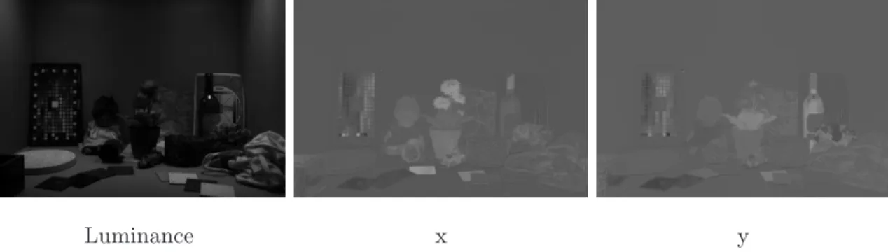
FIG. 5: Luminance and chromaticity estimates of the Little Lucie D65 image, computed from the raw data of a D200 Nikon camera. The normalized luminance image looks dark because of the specular reflection on the bottle.
observer LMS S(O) HVS model display world image RGB RGB sensor model display model XYZ XYZ comparison image processing sensor Iw Id
FIG. 6: The image pipeline: comparison of the Iw and Idimages.
to a, which leads to:
MT[R, G, B]T = (MTM+ qI)a (4)
(I is for the Identity matrix), and finally:
T= N(MTM+ qI)−1MT (5)
For each matrix, we computed a mean error, comparing the computed (x, y) colors of the 180 patches of the Color Checker to the estimated (x, y) colors of the same patches in the image. This was done for the five Little Lucie raw images (with the five light sources). Using q = 1 (T is not very sensitive to q), we found that the best basis for the five light sources corresponds to the D200 RGB sensibility functions. It means that the T matrix
is build assuming that the input spectra are linear combinations of the sensor sensitivity curves (Fig. 4, right). In the following, we use the T matrix computed from these functions:
T= kL 99.086 20.185 8.472 42.821 73.659 −14.630 4.156 −13.290 123.251 (6)
where kL is a luminance normalization factor. Measuring the white patch luminance in the
chart allows to compute this factor without knowing the camera settings (shutter speed, aperture, etc.). For instance, we found kL = 8.22 for the D65 Little Lucie image. Fig. 5
shows the XYZ estimation, with this matrix, for the D65 raw image.
C. Estimation of the Display Output
Display devices expect, as input, the sensor output data, i.e. an array of digital values on RGB channels. The display technology (CRT, LCD, DLP, etc.) transforms these digital values into displayed luminance and chromaticities. The perception of such images depends on geometric conditions (e.g. pixel angular size) and lighting conditions (e.g. surround luminance).
In the proposed framework, the key point is to estimate the photometric and colorimetric properties of the image which is actually seen by an observer. The displayed image Id is
described in XYZ units, as was the world image Iw, allowing further comparison (see Fig. 6).
A photometric and colorimetric calibration of the display device is needed [61, 62], measured in a situation as close as possible to the viewing conditions. Thus, the display device model allows to compute the displayed XYZ signal from the RGB digital values at each pixel. For simplicity reasons, we used a Gain-Offset-Gamma model:
X − X0 Y − Y0 Z − Z0 = xR yR xG yG xB yB 1 1 1 zR yR zG yG zB yB gRRγR gGGγG gBBγB (7)
where (X0, Y0, Z0) is the offset, γk the gamma factors, gk the gain and (xk, yk) the
chro-maticity of channel k (we denote zk = 1 − (xk+ yk) in Eq. 7 for easier reading). We call D
[X, Y, Z]T = [X
0, Y0, Z0]T + D[RγR, GγG, BγB]T (8)
D. Application: NEC 1701 LCD Monitor
The 12-bit raw images from the Nikon D200 (section III B) are processed by the camera firmware, leading to 8-bit JPEG images. Next, these images are displayed on a NEC 1701 LCD monitor, which was characterized in our laboratory, so that a Gain-Offset-Gamma model could be applied to the RGB data in order to estimate the XYZ displayed values of Id (see Fig. 7). We used the following matrix D:
D= 74.95 51.39 24.62 38.90 107.09 11.35 11.56 15.47 134.56 (9)
with γR= 2.80, γG = 2.99 and γB = 2.97. The luminance of the black is 0.4 cd/m2.
Luminance x y
FIG. 7: Luminance and chromaticity estimates of the Little Lucie D65 JPEG image displayed in a dark room on a NEC 1701 LCD monitor.
Fig. 7 shows the same physical components as in Fig. 5 for the displayed image. A direct comparison of these luminance and chromaticity images is not straightforward, as it depends on the media (monitor, printed paper, etc.), so that perceptual metrics are needed. However, some differences are visible, such as the light reflection on the wine bottle which is attenuated in the displayed JPEG image.
Note that without sensor and display calibration, computing error maps between Iw and
transfer matrices:
Iw− Id= kLT[R, G, B] − ([X0, Y0, Z0]T + D[RγR, GγG, BγB]T) (10)
so that Iw = Id is impossible in the general case (see the T and D matrix values Eq. 6 and
9).
IV. HVS-BASED IMAGE QUALITY METRICS
A. Components of Image Quality
Current HVS-based image quality metrics use models of the HVS which take into account a limited part of human vision, thus evaluate the image quality in terms of the selected visual process. For instance, the VDP uses a CSF model, a TVI and a visual masking model, while the CIECAM02 is a Color Appearance Model.
These vision models are validated against psychophysical data. However, the lack of a global HVS model in the current state of the art in vision science leads to a specific problem for HVS-based image quality metrics: one cannot expect that a single HVS model would account for all dimensions of image quality [63].
We propose to cope with this limit using a multi-components description of the image fidelity to the actual scene, taking into account three key issues in human vision which are image-based (making them relevant for an image quality metric). This framework addresses various aspects of human vision in natural situations, however without any bias due to the task or semantic image content. The last restriction applies, to our sense, to any future HVS-based image quality metric, because whatever these task-dependent biases, they are the same in the “world” reference condition and in the “display” condition.
We used three criteria in subjective and objective aspects of the human visual behavior as a basis for image quality metric selection; however we do not claim that more criteria should not be added to these. In sections IV B, IV C and IV D, specific models are chosen for each of these components. They may be replaced by more accurate models without changing the framework. The three image quality criteria are as follows:
1. Observers see the same things in the reference situation (the real world) and in the displayed situation. That is to say, no significant difference is found when comparing between what observers see/fail to see in images Iw and Id.
2. The reference and displayed images look the same to the observers. That is to say, no significant difference is found between the appearance of Iw and Id, as far as observers
can judge.
3. Observers look at the same things in the reference situation and in the displayed image. That is to say, no significant difference is found when comparing gaze positions in Iw and Id. visual appearance model Iw Id visual performance model visual attention model
Error map : VPI
Error map : VAI
Error map : VSI
FIG. 8: Framework of the comparison between the “world” image Iw and the displayed image Id
using three quality indexes: a visual performance index (VPI), a visual appearance index (VAI) and a visual saliency index (VSI).
From these visual behavior components, 3 indexes are proposed, derived from vision models and allowing to compute error maps from Iw and Id (Fig. 8).
1. The Visual Performance Index (VPI) refers to visual performances in a psychophysical sense, such as visibility. This index should take into account, as far as possible, data about the CSF, TVI, visual masking, visual adaptation, mesopic vision, disability glare, etc. Indexes computed from [1, 8, 15, 17, 25, 27, 64] are relevant here.
2. The Visual Appearance Index (VAI) refers to human judgments in a psychophysical sense, such as about brightness and color. The most popular model of this kind is the CIECAM02 [2], however other approaches are possible, such as iCAM [21], brightness
rendering [9], visual equivalence [19], or combining the many “nesses” of images quality through psychometric scaling [38].
3. The Visual Saliency Index (VSI) refers to the image-based bottom-up aspects of visual attention. Indexes computed from [3, 11, 65] are relevant here.
We give evidence in the following that these 3 components of the visual behavior are poorly correlated. Each index emphasizes one aspect of image fidelity. To illustrate these differences, we selected 3 partial models of the HVS in order to build the indexes. We used Daly’s VDP for the visual performance index, CIECAM02 for the visual appearance index and Itti’s saliency map for the visual attention index, given that these models are broadly accepted and used in the image community, and validated against psychophysical data. We do not mean to rate these models, only to propose an implementation of our theoretical framework.
Global indexes may be computed from the local indexes through a spatial summation, e.g. mean square error, mean absolute difference, or any Minkowski metric. However, we follow Daly’s opinion [8] that this spatial summation is a hazardous step.
B. Visual Performance
We use Daly’s VDP as a Visual Performance Index [8], in its HDR version [1]. This model takes as input two luminance images (color information is not processed), and produces a map in which a pixel value is understood as the probability that the difference between the two images at this pixel is visible. The HDR-VDP [1] is a recent evolution of Daly’s model, which may be considered as the reference benchmark for this class of models. It extends the VDP to High Dynamic Range images, including High Contrast vision psychophysical models to the previous framework.
The computation follows several steps: the first one uses an Optical Transfer Function (OTF) to model the light diffusion in the retina, and converted in Just Noticeable Differ-ence (JND) units. This first step models the non-linearity of the HVS. The second step is a Contrast Sensibility Function (CSF) filter. The cortex transform (modified from [16]) creates a multi-channel representation of the image, using radial and orientation filters. Psy-chophysical data modeling visual masking is also taken into account [32]. The last step uses
a psychometric function [66] in order to compute detection probabilities for each sub-band, and the final probability is computed from the partial detection probabilities.
C. Visual Appearance
The Visual Appearance Index is computed from the newest generation of the CIECAM models, the CIECAM02 [2]. It is a consensus among TC 8-01 expert group of the CIE, aiming to predict the color appearance. The model needs some inputs: surround luminance (average, dim or dark), adaptation luminance, and white point in the “world” and “display” conditions. The perceptual attribute correlates are the hue angle h, eccentricity factor e, hue composition H, lightness J, brightness Q, chroma C and saturation s, while a and b give a Cartesian color representation. From these attributes, Luo et al. [67] computed a perceptive color difference:
∆E′ =p(∆J′)2+ (∆a′)2+ (∆b′)2 (11)
where J′, a′ and b′ are derived from J, a and b. In the following, the visual adaptation and
the reference white, which are needed to compute the CIECAM color attributes, are set respectively to the mean color in the image, and to the color of the white patch in the chart (when present) or to five times the mean color otherwise (see [68]).
D. Visual Attention
The Visual Saliency Index is computed using Itti et al.’s saliency map [3]. Like other com-putational models of visual attention, this algorithm uses RGB inputs which are combined in order to compute luminance and opponent colors channels. Thus, we used an analogy between the RGB channels and the physiological LMS channels. The physiological encoding of color in the magno-, parvo- and koniocellular pathways may be described in terms of M+L for the luminance (magnocellular) channel, L-M for the red-green (parvocellular) channel, and S-(M+L)/2 for the blue-yellow (koniocellular) channel [69]. Thus, we computed the LMS values from the XYZ values using the CIECAM02 matrix:
L M S = 0.7328 0.4296 −0.1624 −0.7036 1.6975 0.0061 0.0030 0.0136 0.9834 X Y Z (12)
and computed the opponent color channels from these LMS values in Itti’s algorithm. The saliency map is understood as a probability distribution across space, thus it is normalized to 1 (this normalization was not included in the original algorithm). Then, the VSI is computed as the absolute difference between the two normalized saliency maps.
E. Model implementation and units
In the following, we use online implementations when available: the HDR-VDP is avail-able from the MPI [70]; a “Saliency Toolbox” for Matlab is availavail-able online [71, 72]; and we implemented the CIECAM02 following Moroney et al. [2] to compute the color attributes in an image, and Luo et al. [67] to compute the color difference (Eq. 11).
The units of these three indexes are heterogeneous: the VPI computes, for each pixel, a value between 0 and 1, meaning a probability of difference detection, while the VAI computes a Just Noticeable Difference (JND) from CIECAM02, with values in [0, ∞[; and the VSI computes an absolute difference, also in [0, 1]. There is no obvious way to compare, neither the units, nor the scales, of these outputs. Thus, building a multi-component index out of these three indexes should take this heterogeneity into account (see section V C). A simpler way to use these indexes is comparing the same index for two conditions.
Coming back to the image pipeline, our image quality evaluation framework compares the “world” image Iw (estimated in section III A from a sensor properties) and the displayed
image Id(estimated in section III C from the display device properties). Both are described in
photometric units. Three error maps are computed, using standard vision models validated against psychophysical data. We compare Iw and Id in terms of Visual Performance, Visual
V. RESULTS
What is the need for a multi-component description of image quality? If the VPI, VAI and VSI indexes would roughly measure the perceptive ”error” between the reference image and the displayed image, they should strongly covariate. Moreover, if these errors were correlated, they should be correlated as errors, i.e. the correlation should be positive, and an error near zero for index i should correspond to an error near zero for index j.
In this section, we give evidence that the indexes co-variation is, at best, small (in the statistical sense of an Effect Size), meaning that the underlying processes of human vision are only weakly related to each other. Thus, the indexes measure truly different quality components, which emphasizes the need for a multi-component description of image quality. Moreover, in many cases, improving the image quality according to one quality index lowers the image quality in the sense of another one (significant negative correlations).
A. Image database
Fifty-two photographs were taken under unknown illumination (both indoor and out-door), but including a luminance reference (see examples on Fig. 9, first raw). The black integrating sphere in these images includes a constant light (240 cd/m2, measured with a
video-photometer Minolta CA-S20W). This trick allowed (the sensor being linear) to com-pute the true luminance for the light source area, using two photographs for each scene, with the light source “on” and “off”. For the CIECAM02, we set the adaptation luminance to the mean luminance, and the white luminance to 5 times the adaptation luminance [68]. The Little Lucie image was added to the image database, which result in a set of 53 images. For each of these 53 images, two images were compared. Iw was build from the raw image
and Id was build from the JPEG image (we used the default compression level, set to 6),
displayed on a LCD monitor. Fig. 9 gives some examples of the VPI, VAI and VSI error maps.
B. Statistical Analysis
The Pearson product-moment correlation coefficient r allows to compare two data sets in search for a possible linear correlation. The Spearmann coefficient ρ, considering ranks
instead of data values, checks for a possible monotonic function explaining the dependence between the variables. Considering two images Iwand Id, Pearson and Spearman coefficients
r and ρ were computed to assess the correlation between two image quality indexes (VPI vs. VAI; VPI vs. VSI or VAI vs.VSI) on this image, at the pixel level.
p-values were computed to see whether these coefficients are significantly greater than 0 (one-tailed test, with a significance criteria set to a = .02 in the following). When relevant (positive and significant correlation), an Effect Size (ES) were computed on the correlation coefficients r and ρ [73]. We considered that in psychophysical science, which is relevant for vision models, a statistical effect may be rated as Small when 0.3 < r ≤ 0.5 (that is, the explained variance is between 9% and 25%), Medium when 0.5 < r ≤ 0.707 (the explained variance is between 25% and 50%) and Large when r > 0.707 (the explained variance is above 50%). We rated a correlation as Not Relevant (NR) when it was significantly lower than .30, in a statistical sense (again, the significance criteria was set to a = .02). Note that the proposed approach is optimistic, as two monotonic functions explaining the data from images A and B have no reason to be identical. However, we show in the following that even this approach does not lead to strong correlations.
The JPEG images size was 1950 × 1308 pixels. Due to computing power issues in the recursive computation of pixel ranking (for the Spearman coefficient computation), we used a sub-sampling of the index data (one pixel over 8 in the horizontal and vertical directions). Thus, the degree of freedom (dof) in the statistical tests was N − 2 = 39607, which is why most tests are significant in the following. The true issue of the statistical analysis is the Effect Size of the correlation (see Tab. I and II).
The first step of the statistical analysis was the computation of Pearson correlation coef-ficients. From the 53 × 3 = 159 r values (53 images × 3 comparisons: VPI/VAI, VPI/VSI and VAI/VSI), we found 97 positive r correlations (45 for the VPI/VAI comparisons, 21 for the VPI/VSI and 31 for the VAI/VSI). Due to the high dof value, only 5 positive r values (out of 97) were not significantly > 0. From the 92 significant positives, no Medium or Large Effect Size (ES) effect was found, in the statistical sense proposed above, and only 17 Small ES were found, that is, correlations explaining at least 9% of the total variance (all 17 for VPI/VAI comparisons).
As expected, the Spearman coefficients most of the time improved the correlation co-efficients and the Effect Size: 116 over 159 positive correlations were found, and all were
VPI vs. VAI VPI vs. VSI VAI vs. VSI
image r ES ρ ES r ES ρ ES r ES ρ ES
Little Lucie 0.325 S 0.194 NR -0.094 Neg -0.103 Neg -0.019 Neg -0.070 Neg indoor 1 0.130 NR 0.101 NR 0.083 NR 0.088 NR 0.054 NR 0.050 NR indoor 2 0.359 S 0.381 S 0.079 NR 0.242 NR 0.063 NR 0.366 S indoor 3 -0.160 Neg -0.279 Neg -0.047 Neg -0.073 Neg 0.029 NR 0.237 NR indoor 4 0.153 NR 0.145 NR 0.038 NR 0.083 NR 0.031 NR 0.282 NR indoor 5 0.198 NR 0.161 NR 0.046 NR 0.022 NR 0.015 NR 0.015 NR indoor 6 0.486 S 0.502 M 0.120 NR 0.370 S 0.096 NR 0.374 S indoor 7 0.353 S 0.401 S 0.077 NR 0.239 NR 0.045 NR 0.367 S indoor 8 0.066 NR 0.079 NR -0.095 Neg -0.186 Neg 0.041 NR 0.251 NR indoor 9 0.232 NR 0.171 NR 0.004 NR 0.174 NR 0.014 NR 0.154 NR indoor 10 0.443 S 0.551 M 0.085 NR 0.259 NR 0.046 NR 0.346 S indoor 11 0.370 S 0.217 NR 0.139 NR 0.103 NR 0.173 NR 0.101 NR indoor 12 -0.135 Neg -0.463 Neg -0.176 Neg 0.118 NR 0.064 NR -0.268 Neg indoor 13 0.190 NR 0.064 NR 0.105 NR -0.005 Neg 0.062 NR 0.327 S indoor 14 0.261 NR 0.240 NR 0.043 NR 0.308 S 0.041 NR 0.160 NR indoor 15 0.411 S 0.461 S 0.082 NR 0.332 S 0.062 NR 0.403 S indoor 16 0.296 NR 0.217 NR 0.107 NR 0.152 NR 0.067 NR 0.255 NR indoor 17 0.293 NR 0.408 S -0.040 Neg 0.305 S -0.024 Neg 0.130 NR indoor 18 0.190 NR 0.059 NR -0.014 Neg -0.025 Neg 0.017 NR -0.099 Neg indoor 19 0.072 NR 0.072 NR -0.069 Neg 0.268 NR -0.032 Neg -0.013 Neg indoor 20 0.363 S 0.460 S 0.036 NR 0.385 S 0.035 NR 0.229 NR indoor 21 0.340 S 0.441 S -0.006 Neg 0.313 S -0.019 Neg 0.340 S indoor 22 0.111 NR -0.037 Neg -0.029 Neg 0.221 NR -0.041 Neg -0.108 Neg
TABLE I: Comparison between the image quality indexes on a database of 53 calibrated images. Pearson and Spearman coefficients r and ρ are computed, as well as the and Effect Size. S: Small. M: Medium. L: Large. NR: Not Relevant. Neg: Negative. Part I: indoor images.
significantly > 0. Still, no Large effect (i.e. explaining more than 50% of the variance) was found, and only 2 Medium effects and 14 Small effects were found for the VPI/VAI com-parisons. Meanwhile, 9 Small effects were found for both the VPI/VSI and the VAI/VSI comparisons (no Medium or Large effect was found for these comparisons). Note that a 100% correlation is expected for ρ when an increasing function maps an error index dataset to the other on a given image.
Negative correlations show that in some cases, the image quality in the sens of one index tend to increase when the image quality, in the sense of another index, decreases. This should not happen if the image quality indexes would rate a general purpose image quality. Moreover, the number of Negative correlations in our database was high. Considering r, we found 8 negative values (out of 53) for VPI/VAI, 32 for the VPI/VSI (more than half
VPI vs. VAI VPI vs. VSI VAI vs. VSI
image r ES ρ ES r ES ρ ES r ES ρ ES
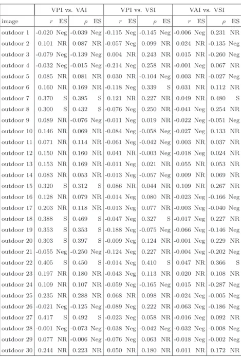
outdoor 1 -0.020 Neg -0.039 Neg -0.115 Neg -0.145 Neg -0.006 Neg 0.231 NR outdoor 2 0.101 NR 0.087 NR -0.057 Neg 0.099 NR 0.024 NR -0.135 Neg outdoor 3 -0.079 Neg -0.139 Neg 0.004 NR 0.243 NR 0.015 NR -0.260 Neg outdoor 4 -0.032 Neg -0.015 Neg -0.214 Neg 0.258 NR -0.001 Neg 0.067 NR outdoor 5 0.085 NR 0.081 NR 0.030 NR -0.104 Neg 0.003 NR -0.027 Neg outdoor 6 0.160 NR 0.169 NR -0.118 Neg 0.339 S 0.031 NR 0.112 NR outdoor 7 0.370 S 0.395 S 0.121 NR 0.227 NR 0.049 NR 0.480 S outdoor 8 0.300 S 0.432 S -0.076 Neg 0.250 NR -0.041 Neg 0.254 NR outdoor 9 0.089 NR -0.076 Neg -0.011 Neg 0.019 NR -0.022 Neg -0.051 Neg outdoor 10 0.146 NR 0.069 NR -0.084 Neg -0.058 Neg -0.027 Neg 0.133 NR outdoor 11 0.071 NR 0.114 NR -0.061 Neg -0.042 Neg 0.003 NR 0.037 NR outdoor 12 0.150 NR 0.160 NR 0.041 NR -0.003 Neg -0.018 Neg 0.024 NR outdoor 13 0.153 NR 0.169 NR -0.011 Neg 0.021 NR 0.055 NR 0.053 NR outdoor 14 0.083 NR 0.053 NR -0.013 Neg -0.057 Neg 0.009 NR 0.069 NR outdoor 15 0.320 S 0.312 S 0.086 NR 0.044 NR 0.109 NR 0.267 NR outdoor 16 0.128 NR 0.079 NR -0.014 Neg 0.080 NR -0.023 Neg -0.166 Neg outdoor 17 0.203 NR 0.118 NR -0.013 Neg 0.077 NR -0.003 Neg -0.040 Neg outdoor 18 0.388 S 0.469 S -0.047 Neg 0.327 S -0.017 Neg 0.227 NR outdoor 19 0.353 S 0.353 S -0.188 Neg -0.075 Neg -0.066 Neg -0.146 Neg outdoor 20 0.303 S 0.397 S -0.009 Neg 0.124 NR -0.001 Neg 0.229 NR outdoor 21 -0.055 Neg -0.250 Neg -0.124 Neg 0.227 NR -0.004 Neg -0.202 Neg outdoor 22 0.405 S 0.450 S -0.014 Neg 0.410 S 0.047 NR 0.366 S outdoor 23 0.197 NR 0.180 NR -0.043 Neg 0.113 NR 0.020 NR 0.108 NR outdoor 24 0.109 NR 0.107 NR -0.059 Neg -0.165 Neg 0.015 NR -0.287 Neg outdoor 25 0.235 NR 0.288 NR 0.068 NR 0.098 NR -0.024 Neg -0.005 Neg outdoor 26 -0.021 Neg -0.125 Neg -0.089 Neg 0.222 NR -0.063 Neg -0.186 Neg outdoor 27 0.417 S 0.492 S -0.023 Neg 0.058 NR -0.016 Neg 0.092 NR outdoor 28 -0.001 Neg -0.073 Neg -0.038 Neg -0.042 Neg -0.032 Neg -0.008 Neg outdoor 29 0.077 NR -0.006 Neg -0.076 Neg 0.063 NR -0.018 Neg -0.002 Neg outdoor 30 0.244 NR 0.223 NR 0.050 NR 0.180 NR 0.011 NR 0.172 NR
TABLE II: Comparison between the image quality indexes on a database of 53 calibrated images. Part II: outdoor images.
the total number of images), and 22 for the VAI/VSI comparisons. For ρ, we found 11 significant negative correlations for VPI/VAI, 14 for VPI/VSI, and 18 for VAI/VSI. Fig. 10 shows images from the database, with various values (both positive and negative) for the indexes correlations.
A specific pattern suggests that the between-indexes correlations are not very consistent. In some cases, we found that rρ < 0, which means that the best linear fit on the index data has a positive slope, while the best linear fit on the rank data has a negative slope (or the
reverse). This situation is anecdotic for the VPI/VAI comparisons (it happens 3 times on 53 image comparisons), but becomes more frequent for the VPI/VSI comparisons (26 times) and for the VAI/VSI comparisons (16 times)
Another pattern emerges, when comparing the 3 image quality indexes: while the corre-lations between VPI/VSI and VAI/VSI are very weak (only 9 Small effects over 53 for both image comparisons, for the Spearman coefficient), the correlation between VPI and VAI is somehow more consistent (16 over 53 images result in a Small or Medium effect size). Our understanding is that these indexes are mainly based on local variations, and uniform areas lead to very small errors both in the VDP framework and CIECAM framework. Conversely, the saliency map tends to select low frequency informations, relevant for peripheral vision, and is thus less sensible to high frequency properties such as local uniformity.
Some limits of the above statistical analysis should be emphasized. First, the analysis was restricted to the image quality indexes correlations, and some expected properties of the indexes were not checked. For instance, a direct computation may show whether, or not, low error values in the sens of one index (say, the 10 first percentiles) occur at pixels with low error values for the other two indexes. Due to the large number of significant negative correlations, we did not feel the need for such a detailed analysis. Another issue is the size of the image database. One may consider that a database of 53 images is quite small, and we agree to some extend. However, we were limited by the fact that a public domain image database was not available with calibrated raw vs. JPEG images. Thus, we had to build the database by ourselves, with a complex protocol, including two photographs with a reference luminance in the field of view (see Section V A). Finally, photographs taken in various situations showed consistent results, with no significant positive Large and only two Medium ES over the 318 computed correlations (r and ρ for the 3 kinds of index comparisons). This quantitative result suggests that even if a larger database of calibrated raw images would improve the present results, the limited size of our database was fair enough for the limited purpose of this paper.
The statistical analysis shows that the VPI, VAI and VSI are only weakly correlated, either using a linear or a non-linear model. This makes sense in terms of visual behavior: the corresponding vision models do not consider the same aspect of vision, and our results show that the 3 selected components of the visual behavior are almost independent. This is more than an intuitive result: the data suggest that these 3 components of the visual
behavior derive from distinct components of the human visual system.
C. A multi-component index
The fact that negative correlations may occur between the three image quality indexes makes it critical for the user to check whether improving one aspect of image quality does decrease image quality as a whole. Therefore, we propose a new index for image quality assessment, based on the previous three [1–3]. In order to get the same range for the three indexes, we have mapped the VAI into [0,1]:
Q = λ1V P I + λ2(1 − e−V AI) + λ3V SI (13)
where (λ1, λ2, λ3) are user-defined parameters, which depend on the application.
VI. CONCLUSION
We have proposed a framework to assess the quality of the Image Acquisition, Process-ing and Display Pipeline, with respect to the visual behavior of observers. We use three components: visual performance is concerned with what is visible in the images, that is, with visibility thresholds; visual appearance is concerned with subjective judgments about the images; and visual attention is concerned with where people look at in the images. The computation of the error maps uses a photometric estimation of two scenes: a reference scene Iw, scanned by a sensor, and a displayed scene Id. The data showed very weak correlations
between the 3 image quality indexes, in terms of Size Effect, calling for a multi-component description of image quality. One such index is proposed, including user-defined parameters. The proposed image pipeline evaluation depends on the reference image (input stimulus) which is chosen for the acquisition step. As the evaluation process depends on the input data, it cannot be said, strictly speaking, that we assess the image pipeline, but rather the pipeline for a given input, which is not suited for most practical applications. In order to extend our approach to a system diagnosis independent of the input data, one may use a reference scene database (rather than an image database), and perform some kind of a benchmark on this database, e.g. with mean indexes over all the reference scenes. Therefore, the development of calibrated raw images databases should be encouraged.
Some recommendations emerge. First, a universal image quality metric seems beyond the range of current knowledge, and possibly unavailable because of the various (and weakly correlated) components of the human visual behavior. Although specific applications of image quality assessment may select a vision model as being more relevant, it may help to check if, for instance, an image processing tuned with respect to this vision model (e.g. visual performance) leads, or not, to drawbacks for alternative quality indexes (visual appearance and visual attention). This was the rationale for the proposed multi-component index.
Second, image quality addresses the fidelity between a displayed image and a physical scene. Assessing one step of the pipeline, as is usually done in image coding evaluation, may loose an important fidelity issue. We suggest to take into account, when possible, the sensor and display characteristics in image fidelity assessment.
Although further developments are necessary in order to include dynamic visual compo-nents to our framework [49, 74], our approach may be useful in the field of TV, movie and video games as well as in vision research. To our sense, the main industrial application is the calibration of a display systems (LCD, plasma, video-projection, printer, etc.) with the knowledge of the image acquisition system properties, allowing to choose the best possible settings in a perceptive sense.
Specific applications may be propose, such as image quality assessment on a specific criterion, while checking the consequences on other quality indexes; Easy calibration settings for display devices, for a better rendering quality in terms of visual perception; Better design of image processing, such as codecs and TMOs, using the knowledge of the acquisition and display devices properties; and of course, direct assessment of the quality of a given image pipeline in terms of visual perception.
Acknowledgments
Thanks to Lucie Br´emond for the baby doll on the picture, Vincent Ledoux for the integrating sphere idea, Roger Hubert and Giselle Paulmier for the photometric and spec-trometric measurements, Josselin Petit for the computations using Itti’s saliency toolbox,
Henri Panjo and Ariane Tom for their help on the statistical analysis.
[1] R. Mantiuk, S. Daly, K. Myszkowski, and H.-P. Seidel, in Proceedings of SPIE Human Vision and Electronic Imaging X (SPIE, 2005), pp. 204–214.
[2] N. Moroney, M. D. Fairchild, R. W. G. Hunt, C. J. Li, M. R. Luo, and T. Newman, in Proceedings of IS&T-SID 10th color imaging conference (2002), pp. 23–27.
[3] L. Itti, C. Koch, and E. Niebur, IEEE Transactions on Pattern Analysis and Machine Intelli-gence 20, 1254 (1998).
[4] S. Nayar and T. Mitsunaga, in Proceedins of IEEE Conference on Computer Vision and Pattern Recognition (2000), vol. 1, pp. 472–479.
[5] H. Seetzen, W. Heidrich, W. Stuerzlinger, G. Ward, L. Whitehead, M. Trentacoste, A. Ghosh, and A. Vorozcovs, ACM Transactions on Graphics 23, 760 (2004).
[6] T. Newman, in Proceedings of the 24th session of the CIE (1999), pp. 5–10. [7] M. P. Eckert and A. P. Bradley, Signal Processing 70, 177 (1998).
[8] S. Daly, The Visible Differences Predictor: An Algorithm for the Assessment of Image Fidelity (A. B. Watson Ed., Digital Images and Human Vision, MIT Press, Cambridge, MA, 1993), pp. 179–206.
[9] J. Tumblin and H. Rushmeier, IEEE Computer Graphics and Applications 13, 42 (1993). [10] M. D. Fairchild, Color appearance models, 2d ed. (John Wiley & Sons, 2005).
[11] L. Itti and C. Koch, Vision Research 40, 1489 (2000).
[12] D. P. Greenberg, K. E. Torrance, P. Shirley, J. Arvo, J. A. Ferwerda, S. N. Pattanaik, E. Lafor-tune, B. Walter, S. C. Foo, and B. Trumbore, in Proceedings of ACM SIGGRAPH (1997), pp. 477–494.
[13] P. G. Engeldrum, Journal of the Imaging Science and Technology 48, 446 (2004).
[14] J. L. Mannos and D. J. Sakrison, IEEE Transactions on Information Theory IT-4, 525 (1974). [15] J. Lubin, A Visual Discrimination Model for imaging system design and development (E. Peli (Ed.) Vision models for target detection and recognition, World Scientific, Singapore, 1995), pp. 245–283.
[16] A. B. Watson, Computer Vision and Image Processing 39, 311 (1987).
600 (2004).
[18] J. A. Ferwerda and D. Pellacini, in Asilomar Conference on Signal, Systems and Computers (2003), pp. 1388–1392.
[19] G. Ramanarayanan, J. Ferwerda, B. Walter, and K. Bala, ACM Transactions on Graphics 26, Art. No 76 (2007).
[20] CIE/ISO, Tech. Rep., CIE publication 131 (1998).
[21] J. Kuang, G. M. Johnson, and M. D. Fairchild, Journal of Visual Communication and Image Representation 18, 406 (2007).
[22] F. Drago, K. Myszkowski, T. Annen, and N. Chiba, in Proceedings of Eurographics (2003). [23] K. Masaoka, M. Emoto, M. Sugawara, and Y. Nojiri, in Proc. SPIE/IS& T Electronic Imaging,
edited by B. E. Rogowitz, T. N. Pappas, and S. J. Daly (SPIE, 2007), vol. 6492, pp. 1F1–1F9. [24] J. Kuang, H. Yamaguchi, C. Liu, G. M. Johnson, and M. D. Fairchild, ACM Transactions on
Applied Perception 4, art. 9 (2007).
[25] M. Ramasubramanian, S. N. Pattanaik, and D. P. Greenberg, in Proceedings of ACM SIG-GRAPH (1999), pp. 73–82.
[26] R. Dumont, F. Pellacini, and J. A. Ferwerda, ACM Transactions on Graphics 22, 152 (2003). [27] S. N. Pattanaik, J. A. Ferwerda, M. D. Fairchild, and D. P. Greenberg, in Proceedings of ACM
SIGGRAPH (1998), pp. 287–298.
[28] J. Stevens and S. Stevens, Journal of the Optical Society of America 53, 375 (1963).
[29] G. Ward, A contrast based scale-factor for image display (Graphic Gems IV, Academic Press Professional, San Diego, CA, 1994), pp. 415–421.
[30] CIE, Tech. Rep., CIE publication 19/2 (1981).
[31] J. A. Ferwerda and S. N. Pattanaik, in Proceedings of ACM SIGGRAPH (1997), pp. 143–152. [32] G. E. Legge and J. M. Foley, Journal of the Optical Society of America 70, 1458 (1980). [33] F. Campbell and J. Robson, Journal of Physiology 197, 551 (1968).
[34] E. Peli, Journal of the Optical Society of America A 7, 2032 (1990).
[35] CCIR, Method for the subjective assessment of the quality of television pictures. Recommen-dation 500-3 (ITU, Geneva, 1986).
[36] H. A. David, The method of paired comparison (Charles Griffin and co. Ltd, 1969). [37] M. P. Eckert, in Proceedings SPIE (1995), vol. 3031, pp. 339–351.
Press, Winchester, MA, 2000).
[39] A. McNamara, Computer Graphics Forum 20, 211 (2001).
[40] G. W. Meyer, H. E. Rushmeier, M. F. Cohen, D. P. Greenberg, and K. E. Torrance, ACM Transactions on Graphics 5, 30 (1986).
[41] P. Ledda, A. Chalmers, T. Troscianko, and H. Seetzen, in Proceedings of ACM SIGGRAPH (ACM, 2005), pp. 640–648.
[42] H. Rushmeier, G. Ward, C. Piatko, P. Sanders, and B. Rust, in Proceedings of Eurographics Rendering Workshop (1995).
[43] J. Grave and R. Br´emond, ACM Transactions on Applied Perception 5, 1 (2008). [44] L. Itti, G. Rees, and J. K. Tsotsos, (Ed.) Neurobiology of attention (Elsevier, 2005). [45] E. I. Knudsen, Annual Review Neuroscience 30, 57 (2007).
[46] C. Koch and S. Ullman, Human Neurobiology 4, 219 (1985).
[47] A. M. Treisman and G. Gelade, Cognitive Psychology 12, 97 (1980). [48] L. Itti, IEEE Transactions on Image Processing 13, 1304 (2004).
[49] L. Itti, N. Dhavale, and F. Pighin, in Proc. SPIE 48th Annual International Symposium on Optical Science and Technology, edited by B. Bosacchi, D. B. Fogel, and J. C. Bezdek (SPIE Press, 2003), vol. 5200, pp. 64–78.
[50] L. Itti and C. Koch, Nature Reviews Neuroscience 2, 194 (2001).
[51] C. H. Lee, A. Varshney, and D. W. Jacobs, ACM Transactions on Graphics 24, 659 (2005). [52] C. Privitera and L. Stark, in Proceedings of SPIE, Human Vision and Electronic Imaging IV
(1999), pp. 552–558.
[53] S. Baluja and D. A. Pomerleau, Robotics and Autonomous Systems 22, 329 (1997).
[54] ISO, Graphic technology and photography. Colour characterization of Digital Still Cameras (DSC) (ISO/WD 17321, 2006).
[55] F. Martinez-Verdu, J. Pujol, and P. Capilla, Journal of Imaging Science and Technology 47, 279 (2003).
[56] S. Mann and R. Picard, in Proceedings of IST 48th annual conference (1995), pp. 422–428. [57] T. Mitsunaga and S. K. Nayar, in Proceedings IEEE Conference on Computer Vision and
Pattern Recognition (1999), vol. 1, pp. 374–380.
[58] A. S. Glassner, IEEE Computer Graphics and Applications 9, 95 (1989).
the Optical Society of America A 25, 2444 (2008).
[60] B. A. Wandell, Tech. Rep. 86844, NASA Ames research center, Moffett Field, CA (1985). [61] CIE, Tech. Rep., CIE publication 122 (1996).
[62] E. A. Day, L. A. Taplin, and R. S. Berns, Color Research and Applications 29, 365 (2004). [63] D. A. Silverstein and J. E. Farrell, in Proceedings of the International Conference on Image
Processing (IEEE, 1996), pp. 881–884.
[64] J. A. Ferwerda, S. N. Pattanaik, P. Shirley, and D. P. Greenberg, Computer Graphics 30, 249 (1996).
[65] J. K. Tsotsos, S. M. Culhane, W. Y. K. Wai, Y. Lai, N. Davis, and F. Nuflo, Artificial Intelligence 78, 507 (1995).
[66] J. Nachmias, Vision Research 21, 215 (1981).
[67] M. R. Luo, G. Cui, and C. Li, Color Research and Application 31, 320 (2006). [68] R. W. G. Hunt, The reproduction of colour, 5th ed. (Fountain Press Ltd., 1995). [69] K. R. Gegenfurtner and D. C. Kiper, Annual Review Neuroscience 26, 181 (2003). [70] MPI, http://www.mpi-inf.mpg.de/resources/hdr/vdp/, Max Planck Institute website. [71] D. Walther, http://www.saliencytoolbox.net/ (2006).
[72] D. Walther and C. Koch, Neural Networks 19, 1395 (2006).
[73] J. Cohen, Statistical power analysis for the behavioral sciences (academic press, 1977). [74] S. Winkler, Digital video quality : vision models and metrics (Wiley, NY, 2005).
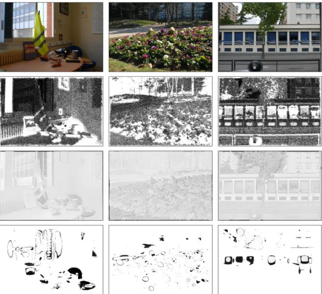
FIG. 9: Normalized error maps computed on sample images from our database, when comparing the reconstructed Iw images and the displayed JPEG Idimages. First raw: JPEG images. Raw 2:
ρ1= 0.38, ρ2= 0.24, ρ3= 0.37 ρ1= −0.28, ρ2= −0.07, ρ3= 0.24 ρ1= 0.50, ρ2= 0.37, ρ3= 0.37
ρ1= 0.55, ρ2= 0.26, ρ3= 0.35 ρ1= −0.46, ρ2= −0.18, ρ3= −0.27 ρ1= 0.46, ρ2= 0.33, ρ3= 0.40
ρ1= −0.04, ρ2= 0.22, ρ3= −0.11 ρ1= −0.14, ρ2= 0.23, ρ3= −0.26 ρ1= 0.08, ρ2= −0.10, ρ3= −0.03
ρ1= 0.39, ρ2= 0.23, ρ3= 0.48 ρ1= 0.08, ρ2= −0.01, ρ3= −0.17 ρ1= 0.47, ρ2= 0.33, ρ3= −0.29
ρ1= 0.11, ρ2= −0.16, ρ3= −0.29 ρ1= −0.07, ρ2= −0.04, ρ3= −0.01 ρ1= −0.01, ρ2= 0.18, ρ3= 0.17
FIG. 10: Spearman Correlation coefficient values when comparing the image quality indexes VPI and VAI (ρ1), VPI and VSI (ρ2), VAI and VSI (ρ3).
![FIG. 1: Standard framework for HVS-based image metrics, such as [8, 14]. In the following figures, yellow boxes refer to images, green boxes refer to image processing and pink boxes refer to human vision components.](https://thumb-eu.123doks.com/thumbv2/123doknet/6057862.152422/3.892.258.659.485.641/standard-framework-metrics-following-figures-images-processing-components.webp)