DAYTIME FOG DETECTION AND DENSITY ESTIMATION WITH ENTROPY
MINIMIZATION
Laurent Caraffaa, Jean-Philippe Tarelb a
IGN, MATIS, 73 Avenue de Paris, Saint-Mand´e.
bIFSTTAR, LEPSiS, 14-20 Boulevard Newton, Cit´e Descartes, Champs-sur-Marne, F-77420 . Paris-Est University, France.
WG VI/4
KEY WORDS: Image processing, fog detection, fog caracterisation, stereo camera
ABSTRACT:
The fog disturbs the proper image processing of many outdoor observation tools. For instance, fog reduces the obstacle visibility in vehicle driving applications. Usually, the estimation of the amount of fog in the scene image allows to greatly improve the image processing, and thus to better perform the observation task. One possibility is to restore the visibility of the contrasts in the image from the foggy scene image before to apply the usual image processing. Several algorithms were proposed in the recent years for defogging. Before to apply the defogging, it is necessary to detect the presence of fog, not to emphasis the contrasts due to noise. Surprisingly, only a reduced number of image processing algorithms were proposed for fog detection and characterization. Most of them are dedicated to static cameras and can not be used when the camera is moving. The daytime fog is characterized by its extinction coefficient, which is equivalent to the visibility distance. A visibility-meter can be used for fog detection and characterization, but this kind of sensor performs an estimation in a relatively small volume of air, and is thus subject to heterogeneous fog, and air turbulence when the camera moves.
In this paper, we propose an original algorithm, based on entropy minimization, to detect the fog and estimate its extinction coefficient by the processing of stereo pairs. This algorithm is fast, provides accurate results using low cost stereo cameras sensor and, the more important, can work when the cameras are moving. The proposed algorithm is evaluated on synthetic and camera images with ground truth. Results show that the proposed method is accurate, and, combined with a fast stereo reconstruction algorithm, should provide a solution, close to real time, for fog detection and extinction coefficient estimation for moving sensors.
1. INTRODUCTION
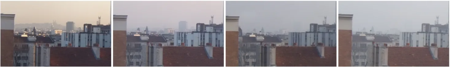
Even if fog is rare, fog impacts the quality of the results of many images processing algorithms when applied on outdoor scenes, see Fig. 1. For example, fog reduces vehicle and obstacle visi-bility when driving, which leads to death injuries. Solutions have been investigated to tackle the problem of reduced visibility when fog is around the vehicle. One possibility is to detect fog, turn on the fog lights and depending of the importance of the fog which is measured by the extinction coefficient β, adapt the strength of the fog lights, as demonstrated in ICADAC project1. An alterna-tive is to display to the driver an image of the scene ahead of the vehicle after visibility restoration by image processing, see for instance (Tarel et al., 2012).
Fog detection and characterization is thus an important question to deal with in these problems. Several algorithms were proposed for defogging, in particular in the recent years. A first class is based on color and contrast enhancement, for instance (Job-son et al., 1997, Zuiderveld, 1994). A second class is based on the Koschmieder’s law to model the effect of the fog, for in-stance (Tan, 2008, He et al., 2010, Tarel and Hauti`ere, 2009, Tarel et al., 2010). With a linear response camera, the Koschmieder’s laws gives the apparent intensity I of an object as a function of its intrinsic intensity I0and of the fog extinction coefficient β:
I= I0e−βD+ Is(1 − e−βD) (1) Thanks to the FUI AWARE project for partial funding.
1ICADAC project (6866C0210) is within the Deufrako program and was funded by the ANR (French National Research Agency).
where D is the object depth, and Isis the intensity of the sky. The ”meteorological visibility distance” is defined conventionally, as a function of β, by:
dvisibility = − ln(0.05)
β (2)
In (Tarel et al., 2012), experiments shows that algorithms based on the Koschmieder’s law generally do better than the ones not based on this law. If most of the time, the value of β is not neces-sary to perform the defogging, one may notice that, when applied to road images, the value of β is necessary to use the planar road assumption. The detection of the fog is also necessary, not to apply defogging methods when it is useless.
Surprisingly only a reduced number of methods were proposed for detecting fog from a camera and for estimating the extinc-tion coefficient β. Most of these methods apply only when the camera is static. The first approach is to estimate the decrease of contrast of far away objects, see for instance (Bush and Debes, 1998, Hauti`ere et al., 2011). In (Kopf et al., 2008), the attenu-ation model due to fog is estimated assuming that a 3D model of the scene is known. This method is interesting since it shows that the Koschmieder’s law is not always valid on long range dis-tances due to heterogeneous fog. The difficulty with this method is that an accurate 3D model is required. When the camera is moving, only three approaches were proposed, the first one is based on the use of lane-markings, the second on the road planar assumption and the third on the use of the stereo. In (Pomerleau, 1997), β is obtained by looking the contrast attenuation of road markings at various distances. The disadvantage of this method is that it requires the presence road markings in order to proceed. In (Lavenant et al., 2002, Hauti`ere et al., 2006b), it is proposed
Figure 1: Contrast fading on the same scene due to various values of the extinction coefficient β.
a method dedicated to in-vehicle applications. This method as-sumes that the road is planar with a homogeneous gray level, and that the camera calibration is known with respect to the road plane. In case of fog, the gray level profile on the road, in the vertical direction, is derived from (1) and it shows an inflection point. The position of this inflexion point can be used to estimate the value of β. The weakness of this method is that several as-sumptions are required for the method to work. Another problem is that the inflexion point may be hidden by a close object in case of a light fog. In (Hauti`ere et al., 2006a), a stereovison approach is proposed. It consists in detecting the most distant object with a contrast above5%. This method is simple but it is requires the presence of objects with high contrasts at every distances, and this is not always the case in practice.
From the drawbacks of the previous fog detection and fog char-acterization methods when the camera is moving, we see that a generic method is needed. We thus proposed a generic method which is based on stereovision. In (Caraffa and Tarel, 2013), a MRF model for stereo reconstruction and defogging is proposed. By minimizing this energy, β can be estimated. However, this approach will lead to a slow iterative algorithm to produce good results. Inspired by (Caraffa and Tarel, 2013), we here investigate the estimation of the extinction coefficient β when an approxi-mate depth map is provided upon a critical distance. We thus assume that a fast stereo reconstruction was first applied and that this algorithm provides enough good matches upon the critical distance. When the depth is known, the main idea is to estimate β from the attenuation of the contrast w.r.t the distance on ho-mogeneous areas in the scene. Similarly to the case of shadows removal (Finlayson et al., 2009, Kwatra et al., 2012), the Shan-non entropy is used as a criterion and the proposed method for estimating β consists in the entropy minimization of the restored image. The advantage of the proposed approach over previous ap-proaches is that it is generic and we do not need the whole range of distances in the depth map. The proposed algorithm, combined with a real time stereo reconstruction algorithm, should provide a fast algorithm for estimating the extinction coefficient (which includes the detection of foggy weather using a threshold on the visibility distance) when the camera is moving. As shown in the experiments, it leads also to accurate results when the camera is static.
First, in section 2., the problem of fog detection and extinction coefficient estimation is explained and our approach is presented. Then, the algorithm is detailed in section 3.. In section 4., the pro-posed algorithm is evaluated on a synthetic database for a moving camera and evaluated with a ground truth database for static cam-era images.
2. PROBLEM STATEMENT
When a region with a uniform albedo is observed in presence of fog, its image is not of constant intensity. Indeed, its image be-comes whiter with an increasing depth. This is due to the last additive term in (1), the so-called atmospheric veil which is an
increasing function of the depth D. The Shanon entropy is a measure of the redundancy of a probability distribution. As a consequence, the entropy of the intensity distribution of a region of constant albedo, i.e without fog, is very small. On the con-trary, the entropy of the same region in presence of fog is larger if the region span a large range of depths. Our main idea is thus to estimate the extinction coefficient β as the value which gives the restored image with the smallest entropy on regions of constant albedo.
The Fig. 2. illustrates the principle of the proposed method. A foggy image is shown in the Fig. 2(a). We search for regions of constant albedo. We thus propose to segment the foggy image in regions where the intensity varies slowly, see Fig. 2(b). Some of the obtained regions, such as the fronto-parallel regions, or the regions with small depth variations are not adequate for the estimation of β and thus must be rejected. Relevant segmented regions are thus selected using a criterion on the region area and on the region depth variations. In Fig. 2(c), this criterion leads to the selection of only three regions. In Fig. 2(d), 2(e) and 2(f), the image after restoration assuming different values of β are shown, respectively with β = 0.0024, β = 0.0086 and β = 0.0167. These restorations are simply obtained by inversing (1), i.e by computing I0, for each pixel, from the foggy image I, from the value of Isand from the depth map D. The correct value for β is the second one, and was obtained using a visibility-meter. We can see that, when β is too small, the restored image is still foggy and the gradient due to fog on homogeneous regions is percepti-ble. Conversely, when β is too large, far away parts of the image become too dark. For the ground-truth value β= 0.0086, the re-stored image is more homogeneous and thus looks better than the others. In Fig. 2(g), 2(h) and 2(i), the gray level distributions on the 3 selected regions are displayed after defogging. We can see, for the correct value β = 0.0086, that the gray level histogram of each region is tighter than for the other values of β. There-fore, the entropy is smaller for this value compared to the two others. Fig. 2(j) shows the entropy of each selected regions ver-sus β. It appears that a minimum of the entropy is reached around the ground-truth value of β for the tree selected regions. Finally, in Fig. 2(k), the total entropy over the three selected regions is displayed versus β. The total entropy on the image is also shown. The previously used values of β are displayed as vertical lines. It is clear from that figure, that the minimization of the sum of the entropy over the selected regions allows to better estimate the value of β by doing an averaging on the three selected regions. The minimum of the sum of the entropy over the selected regions is very close to the ground truth value. On the contrary, the en-tropy over the image does not lead to a good estimate. Indeed, the entropy over the image intensities is mixing several random variables and can not be a coherent choice.
3. ALGORITHM
The used sensor is stereo cameras. For every stereo pair, the stereo reconstruction is performed by one or another method. The choice of the stereo reconstruction algorithm is studied in the next
(a) Foggy image (b) Segmentation (c) Selected regions
(d) Restoration with β = 0.0024 (e) Restoration with β = 0.0086 (f) Restoration with β = 0.0167
0 0.1 0.2 0.3 0.4 0.5 0.6
0 5000 10000
(g) Gray level histogram of the restoration with β = 0.0024
0.1 0.2 0.3 0.4 0.5 0.6
5000 10000 15000
(h) Gray level histogram of the restoration with β = 0.0086
0 0.1 0.2 0.3 0.4 0.5 0.6
0 5000 10000
(i) Gray level histogram of the restoration with β = 0.0167
β Entr opy 0.005 0.01 0.015 0.02 0.025 4 4.5 5 5.5 6
(j) Entropy as function of β for the 3 selected regions
β Entr opy (%) 0.005 0.01 0.015 0.02 0.025 0 0.2 0.4 0.6 0.8
Full image entropy
Sum of segmented zones entropy
(k) Sum over the 3 selected regions of the entropy and image entropy
Figure 2: Variation of the entropy with and without segmentation for different value of β. On the first line, 2(a) is the foggy image where the ground-truth is known: β = 0.0086, 2(b) is the used segmentation and 2(c) are the three selected regions. On the second line are the restored images for different value of β, when the depth-map D is known. Next, the gray level histograms of the intensity distribution on the selected regions are shown for three different values of β. Then, 2(j) shows the entropy of the three selected regions versus β and 2(k) shows the sum over the selected regions of the entropy compared to the image entropy. In the last figure, vertical lines displays the value of the three β values used previously.
section experimentally, where it is shown that the stereo recon-struction only needs to be correct in a relatively short range of distances close to the cameras. The input of the proposed fog detection and characterization algorithm are thus an input cam-era image I(x) observed with or without atmospheric scattering and the corresponding depth map D(x) obtained from the stereo reconstruction.
When I(x) and D(x) are known, in the equation (1), the extinc-tion coefficient β , the restored image I0and the intensity of the sky ISremains unknown. The first step of the algorithm is thus to estimate ISin an original way. Then, given a β, the restored im-age I0can be computed by solving (1). The second step consists in searching the value of β which minimizes the total entropy of the gray level distributions over selected regions of the restored image.
3.1 Estimation of IS
In defogging methods, the intensity of the sky is usually obtained using simple methods such as the selection of the maximum in-tensity in the image, or as the value corresponding to a given quantile on the intensity histogram, see for instance (Tan, 2008, Tarel and Hauti`ere, 2009). If this kind of approach gives approx-imate results in practice, we observed that an accurate ISis im-portant to estimate correctly the value of β. In particular, the fog being not necessarily homogeneous on long range distances, it is necessary to estimate a correct value of the ISin the close sur-rounding of the camera.
We thus introduce a first novel and simple method, based on con-trast detection using the Sobel operator to estimate IS. First, we compute the Sobel operator on the input image. Second, pixels with a gradient magnitude larger than an arbitrary threshold are selected. Third, we chose ISas the highest intensity value in the vicinity of the pixels selected by the gradient thresholding. This previous method can be applied on static or moving cameras. When the depth-map of the observed scene is known with enough accuracy, in particular when the scene is static, a little better can be done. In such a case, the value of IS can be estimated by taking the maximum intensity at the farthest distance detected by the pixels selected by the gradient thresholding. This refined method gives better results as shown in the experiments. 3.2 Region selection
The entropy minimization is meaningful only on a set of regions with constant albedo and with varying enough depths. The in-put image is thus segmented in regions where the intensity varies slowly. The regions with constant intensity or fronto-parallel to the image are rejected as well as the tiny regions which are use-less. The used criterion for this selection is to select regions with a depth range higher than10% of the whole image depth range and with an area higher than2% of the number of image pixels. This segmentation can be performed with advantages on a clear day image when a static sensor is used. The segmentation can be also performed on both the image and the depth map, when the depth map is enough accurate.
3.3 Estimation of β and I0
Once ISis estimated, I0can be obtained for a given β by solving equation (1). To measure the quality of the restored image I0, we use the Shannon formulation of the entropy defined for a random variable y ∈ Y :
H(Y ) = −E[log p(y)] = −X y∈Y
p(y) log p(y) (3)
where E is the expectation function and p(y) is the probability density function of variable y. The entropy is defined for a sin-gle random variable, but for several independent variables, the entropy of the set of these variables is the sum of the individual entropy.
Actual scenes are composed of many objects, and thus its image is composed of several regions, and each region have its own ran-dom variable. Let Scthe set of selected regions in the previously described step. The total entropy is thus computed on this set of selected region as:
T H= X Yi∈Sc H(Yi) = − X Yi∈Sc X y∈Yi
p(y) log p(y) (4)
The total entropy is computed for a set of possible β values, and the estimate of β is obtained as the value minimizing the total entropy (4). This computation is quite fast, since only pixels in the selected region with valid depths need to be considered and restored.
Due to wrong estimates in the depth map, due to heterogeneous fog, the intensity after restoration can be saturated and becomes black. This case appears for the ground-truth value of β= 0.0001 in the Fig. 3(e) where remote objects are black on the right of the image. This is due to the fact that the fog is lighter in this area. Not to be perturbed by this saturation, a maximal percent-age of black pixels is allowed and β values with restorations with a larger percentage are discarded.
3.4 Summary
To resume, the proposed algorithm is the following:
• Detection of the pixels with a gradient magnitude higher than a threshold on the input intensity image I(x). IS is set as the highest intensity in the vicinity of these detected pixels.
• Segmentation of I(x) in regions and selection of the reliable regions Scby a threshold on the depth range and on the area. • For each β, in a set of possible increasing values:
– Compute the restored image for the pixels in the se-lected regions Sc, when the depth map D(x) is known, using:
I0(x) = I(x)eβD(x)−IS(eβD(x)−1) – Compute the total entropy T H over the segmented
re-gions of the restored intensity distributions I0 using (4).
– Count the number of black pixels in the restored im-age I0, and if this number is higher than a threshold, the search on higher β values is stopped.
• The solution is given as the value of β which minimizes the total entropy (4).
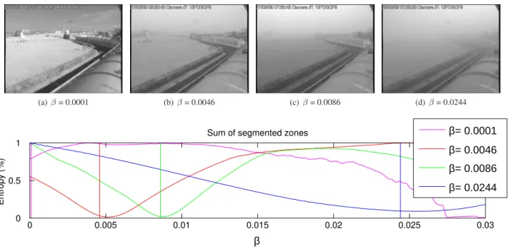
In Fig. 3, the total entropy on the three selected regions is shown versus the value of β. The ground-truth β values are shown as vertical lines. This figure shows how the ground-truth is close of the minimum of the total entropy, in various weather conditions.
(a) β = 0.0001 (b) β = 0.0046 (c) β = 0.0086 (d) β = 0.0244
Sum of segmented zones
β Entro py (%) 0 0.005 0.01 0.015 0.02 0.025 0.03 0 0.5 1 β= 0.0001 β= 0.0046 β= 0.0086 β= 0.0244
(e) Sum of selected regions entropy on the four images
Figure 3: Normalized total entropy versus β on the same scene with different weather conditions. The ground-truth β measured with a visibility-meter are shown (0.0001, 0.0046, 0.0086 and 0.0244) as vertical lines.
3.5 Complexity
Computing the entropy of each intensity is linear according to the number of pixel. If β has K possible values and the image N pixels, The complexity of the proposed algorithm is O(KN ). The proposed algorithm can be easily parallelized. Indeed, the restored image for each beta can be computed independently and the entropy can be computed with a map-reduce approach.
4. EVALUATIONS
To evaluate the proposed algorithm, we need foggy images with a visibility distance ground-truth. A visibility-meter can be used for the ground-truth. However and until now, we are not able to have moving stereo images of foggy scenes with a ground-truth. Indeed, the measures obtained by a visibility-meter are very perturbed by air turbulence around the sensor when it is on a moving vehicle. This is probably due to the fact that a visibility-meter uses a relatively small volume of air for its measure. As a consequence, we rely on synthetic images to experiment with moving scenes. For static scene, we rely on camera images. 4.1 Static sensor
The input of the proposed algorithm being an intensity image and a depth-map, we evaluated it using the Matilda database intro-duced in (Hauti`ere et al., 2011). The Matilda database provides a sequence of more than 300 images from a static low cost cam-era during three days (night and day) with the visibility distances from a visibility-meter. An approximate depth map of the scene is also provided. In this database, the visibility varies from100m to15km, and the accuracy of the used visibility-meter is around 10%. The maximum distance in the depth map is 1300m. To challenge the proposed algorithm, we also performed tests where the image is processed in a reduced range of depths. Thus, the evaluation results are presented in two cases: in the first case, all the depth map is used (denoted Dmax(IS)), and in the sec-ond case, only the pixels with a depth lower than 50m are used
Range (m) 0-250 0-500 0-1000 all
number of images 9 19 24 198
Single image segmentation
Dmax(IS) 10.0% 9.1% 11.7% 97.3% Dmax= 50m 7.1% 7.1% 10.0% 91.5%
Images segmentation
Dmax(IS) 25.4% 17.2% 20.7% 101.7% Table 1: Mean relative error between the estimated visibility dis-tance and the ground-truth on the Matilda database for different distance ranges, with a single image segmentation. The first line is obtained from the maximum distance Dmaxwhere IS is ob-served and the second line is for a shorter and fixed distance Dmax = 50m. On the last line, the segmentation is computed on every image, to simulate the situation of embedded sensors in a moving vehicle.
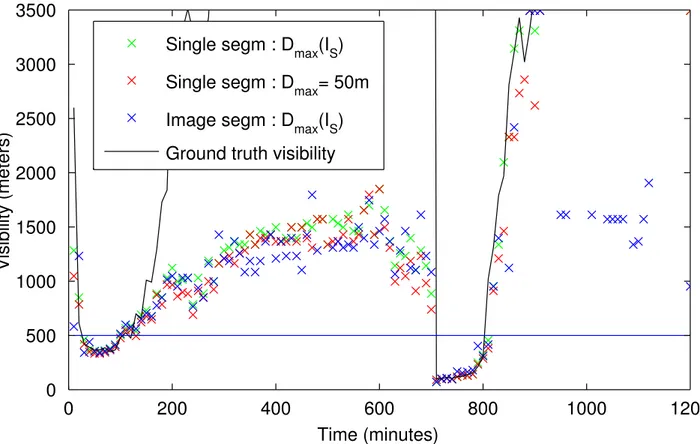
(denoted Dmax = 50m). The camera being static, the segmen-tation in region is performed a single time on an image with clear weather conditions using the algorithm proposed in (Felzen-szwalb and Huttenlocher, 2004). We thus use the same selected regions for all the proceeded images in the sequence. This al-lows to evaluate the visibility distance estimation without the ex-tra source of errors due to the segmentation process. The effect of applying the segmentation on every image is also tested. Tab. 1 shows the evaluation results in term mean relative error on the visibility distance. We can see that the algorithm produces results with a similar accuracy than the visibility-meter, up to 1000 meters. Notice that results are even better when the dis-tance range is limited to50 meters. This can be explained by the fact that fog is not always homogeneous, and a short range allows to better fit the ground-truth which is measured close to the cam-era. In these experiments, the second variant on the ISestimation is used to achieve better results. Fig. 4 shows the results during two foggy in the morning days, with an image every 10 minutes, night images are skipped. These results show that the proposed algorithm is able to clearly discriminate between visibility dis-tance lower or higher than500m. The distance were fog is no
Time (minutes)
Visib
ility (m
eters)
0
200
400
600
800
1000
1200
0
500
1000
1500
2000
2500
3000
3500
Single segm : D
max(I
S)
Single segm : D
max= 50m
Image segm : D
max(I
S)
Ground truth visibility
Figure 4: Comparison between estimated visibility distance and ground-truth during 1600 minutes (one image every 10 minutes, images during the night are skipped) on the Matilda database. The proposed method is tested with two depth ranges: maximum distance where ISis obtained (green crosses) and a fixed range[0, 50]m (red crosses), using a single image segmentation and is also shown the case with a different segmentation at every image (blue crosses). The ground-truth value is shown as a black line. The horizontal blue line shows the500m visibility distance which is considered as the distance were fog is no more considered in driving situations.
With ground truth distance Mean relative error 4.67% With stereo reconstruction depth map Mean relative error 16.03%
Table 2: Mean relative error between the estimated visibility dis-tance and the ground-truth value on 66 synthetic stereo images from Frida3 database. In the top part, the ground-truth depth-map is used and in the bottom part, the depth-depth-map comes from the stereo reconstruction using Libelas algorithm.
more considered in driving situations is500m. 4.2 Moving sensor
In the case of a moving sensor, we evaluate the proposed method on66 synthetic stereoscopic images with uniform fog from the database named Frida3. This database was introduced in (Tarel et al., 2012) for stereo reconstruction and restoration evaluation and contains a ground-truth: the images without fog and the as-sociated depth-maps.
To study the effect, on the estimated β, of bad matches in the stereo reconstruction, we compared the case where the ground-truth depth-map is used with the case where the depth-map comes from a fast stereo reconstruction algorithm. In practice, we use the Libelas algorithm which is very fast and is dedicated to road scene images (Geiger et al., 2010). Tab. 2 shows the obtained results in terms of mean relative error on the estimated visibility distance in the two cases. Results obtained using the ground-truth
depth-map are very accurate, when the stereo reconstruction is used, accuracy is lower but still of good quality.
5. CONCLUSION
In this article, we propose an original method for estimating the extinction coefficient of the fog or equivalently the meteorolog-ical visibility distance. The proposed method is based on the entropy minimization of the restored image on pixels where the depth is known. The depth-map can come from a 3D model of the scene, or from a stereo reconstruction as well. The results obtained on a static scene are as accurate that what is usually obtained with a visibility-meter, when the depth-map is of good quality. The proposed algorithm can be also used with a moving sensor and is tested with success on synthetic stereo images. The proposed algorithm have several advantages. First, a small depth range can be used to characterize a visibility distance 10 times larger than the maximum depth in the depth-map. This is impor-tant for vehicular applications where obstacles or other vehicles can hide a large range of distances. Another important conse-quence is that the used stereo reconstruction algorithm needs to provide good matches only up to a critical distance which is much lower than the visibility distance. Second, the proposed method is close to real time and it is fast enough to investigate real-time applications for vehicular applications. In particular, it can be easily speed-up using parallel computations.
REFERENCES
Bush, C. and Debes, E., 1998. Wavelet transform for analyzing fog visibility. IEEE Intelligent Systems 13(6), pp. 66–71.
Caraffa, L. and Tarel, J.-P., 2013. Stereo reconstruction and con-trast restoration in daytime fog. In: Proceedings of Asian Con-ference on Computer Vision (ACCV’12), Part. IV, LNCS, Vol. 7727, Springer, Daejeon, Korea, pp. 13–25.
Felzenszwalb, P. F. and Huttenlocher, D. P., 2004. Efficient graph-based image segmentation. Int. J. Comput. Vision 59(2), pp. 167–181.
Finlayson, G. D., Drew, M. S. and Lu, C., 2009. Entropy min-imization for shadow removal. Int. J. Comput. Vision 85(1), pp. 35–57.
Geiger, A., Roser, M. and Urtasun, R., 2010. Efficient large-scale stereo matching. In: Asian Conference on Computer Vision, Queenstown, New Zealand.
Hauti`ere, N., Babari, R., Dumont, E., Br´emond, R. and Paparo-ditis, N., 2011. Estimating meteorological visibility using cam-eras: a probabilistic model-driven approach. In: Proceedings of the 10th Asian conference on Computer vision - Volume Part IV, ACCV’10, Springer-Verlag, Berlin, Heidelberg, pp. 243–254. Hauti`ere, N., Labayrade, R. and Aubert, D., 2006a. Estimation of the visibility distance by stereovision: A generic approach. IEICE Transactions 89-D(7), pp. 2084–2091.
Hauti`ere, N., Tarel, J.-P., Lavenant, J. and Aubert, D., 2006b. Au-tomatic fog detection and estimation of visibility distance through use of an onboard camera. Machine Vision and Applications 17(1), pp. 8–20.
He, K., Sun, J. and Tang, X., 2010. Single image haze removal using dark channel prior. IEEE Transactions on Pattern Analysis and Machine Intelligence 33(12), pp. 2341–2353.
Jobson, D. J., Rahman, Z. U. and Woodell, G. A., 1997. A mul-tiscale retinex for bridging the gap between color images and the human observation of scenes. IEEE Trans. Image Process-ing 6(7), pp. 965–976.
Kopf, J., Neubert, B., Chen, B., Cohen, M. F., Cohen-Or, D., Deussen, O., Uyttendaele, M. and Lischinski, D., 2008. Deep photo: Model-based photograph enhancement and view-ing. ACM Transactions on Graphics (Proceedings of SIGGRAPH Asia 2008) 27(5), pp. 116:1–116:10.
Kwatra, V., Han, M. and Dai, S., 2012. Shadow removal for aerial imagery by information theoretic intrinsic image analysis. In: International Conference on Computational Photography. Lavenant, J., Tarel, J.-P. and Aubert, D., 2002. Proc´ed´e de d´etermination de la distance de visibilit´e et proc´ed´e de d´etermination de la pr´esence d’un brouillard. French pattent num-ber 0201822, INRETS/LCPC.
Pomerleau, D., 1997. Visibility estimation from a moving vehicle using the ralph vision system. IEEE Conference on Intelligent Transportation Systems pp. 906–911.
Tan, R., 2008. Visibility in bad weather from a single image. In: IEEE Conference on Computer Vision and Pattern Recognition (CVPR’08), Anchorage, Alaska, pp. 1–8.
Tarel, J.-P. and Hauti`ere, N., 2009. Fast visibility restoration from a single color or gray level image. In: Proceedings of IEEE In-ternational Conference on Computer Vision (ICCV’09), Kyoto, Japan, pp. 2201–2208.
Tarel, J.-P., Hauti`ere, N., Caraffa, L., Cord, A., Halmaoui, H. and Gruyer, D., 2012. Vision enhancement in homogeneous and het-erogeneous fog. IEEE Intelligent Transportation Systems Maga-zine 4(2), pp. 6–20.
Tarel, J.-P., Hauti`ere, N., Cord, A., Gruyer, D. and Halmaoui, H., 2010. Improved visibility of road scene images under heteroge-neous fog. In: Proceedings of IEEE Intelligent Vehicle Sympo-sium (IV’2010), San Diego, California, USA, pp. 478–485. Zuiderveld, K., 1994. Contrast limited adaptive histogram equal-ization. In: P. S. Heckbert (ed.), Graphics gems IV, Academic Press Professional, Inc., San Diego, CA, USA, pp. 474–485.