Control and simulation of doubly fed induction generator
for variable speed wind turbine systems based on an
integrated finite element approach
Qiong-zhong Chen*, Michel Defourny#, Olivier Brüls* * University of Liège,
Department of Aerospace and Mechanical Engineering (LTAS) Chemin des Chevreuils 1 (B52/3), 4000 Liège, Belgium
Email: [email protected], [email protected] #
SAMTECH Headquarters, Liège science park,
Rue des Chasseurs-Ardennais 8, 4031 Liège (Angleur), Belgium Email: [email protected]
Abstract:
Regarding renewable energy and environment- friendly issues, wind energy nowadays has become the fastest-growing energy source in the world, and thus attracts a lot of research interest in the wind turbine generation system. A doubly fed induction generator (DFIG) is used for variable speed operation in a wind turbine system to extract more power. Following a systematic approach, this paper investigates on the modelling and simulation of wind turbine generating systems using the flexible multibody simulation software SAMCEF/MECANO [1]. The objective of this work is to analyze the control-generator-structure interactions in a wind turbine system. Firstly, an extension of the finite element method is integrated into the flexible multibody dynamics solver, and thus extends the solver to represent mechatronic systems in a strongly-coupled way. Secondly, DFIG and the control systems are modularly modeled for the wind turbine package. Control of DFIG for grid synchronization and power optimization are elaborated in detail, and the methods are validated through a 2MW DFIG wind turbine prototype model. At the end, a systematic system model of wind turbine structure connected with the DFIG generating system is presented, which provides the dynamic analysis for the whole system in an overall range.
Keywords: DFIG, wind turbines, control,
strongly-coupled finite element approach
1 Introduction
As one of the most promising renewable energy sources, wind power has substantially increased for the past decade and is evaluated as the best choice to fill the electricity generation gap according to the published findings by the International Energy Agency (IEA) in 2006. A wind turbine system is used
to convert wind energy into electrical energy. For a given turbine blade airfoil, the power extracted from an air stream depends on the wind speed, the air density and also the turbine rotating speed. Since wind cannot be controlled, turbine rotating speed is then controlled for optimizing wind power extraction. Therefore, a variable-speed wind turbine is of higher energy efficiency than fixed-speed wind turbines. Besides, variable speed operation can reduce mechanical stress on turbine structure and is claimed to be better for acoustic noise reduction [2]. Variable-speed wind turbines are typically based on a doubly-fed induction generator (DFIG), which can operate over a slip range of +/-30% and thus enable the turbine to extract the maximum power from the wind with variable operating speeds. One important advantage of DFIG in the applications of wind turbines, especially large-power wind turbines, is that only a slip power, typically 20-30% of the total power, has to be handled by the bidirectional rotor converter. Consequently, both the power rating requirement and losses can be highly reduced.
For the control of a wind-turbine-driven DFIG, different strategies like direct torque control (DTC) and variable structure control (VSC) have been proposed over the last decade [3]. However, one common way is to use vector control on the basis of
d,q-transformation with stator-flux orientation or
stator-voltage orientation (also referred to as grid-voltage or grid-flux orientation) [4]. Typically, two ways can be used for vector control schemes. One is by means of integral-proportional (IP) regulators and the other is by proportional-integral (PI) regulators. The difficulty then lies in the configuration and the determination of the coefficients of the regulators. Since a wind turbine system is a hybrid system featuring not only mechanical structures, but also aerodynamics, control systems and the coupling interaction in-between. Computer-aided tools
provide a way to reduce cost and improve efficiency in the design of wind turbine systems. While specializing on the mechanical structure and the motion, most commercial finite element method (FEM) based wind turbine softwares can be extended to represent non-mechanical systems by implementing a user-element in a weakly-coupled way, which means that specific solvers are used for control systems and mechanical subsystems respectively, and data are exchanged only at particular communication times [5]. However, since the dynamics of the actuators or generators are continuous in time, weakly-coupled approaches could lead to large numerical errors if the time steps are not set small enough. This method might be quite intricate in applications, and sometimes even unreliable. On this account, the development of an integrated flexible multibody dynamics solver based on a strongly-coupled method would be important for achieving better reliability and efficiency.
Among the wind turbine softwares, Samcef for Wind Turbine (S4WT) is based on the flexible multibody dynamics solver Samcef/Mecano [1]. Funded by the Walloon government, Samtech and the University of Liège are jointly engaged to develop and improve the wind-tubine software package S4WT under the project Dynawind. The general aim is to develop a computer-aided tool for customization, fast- prototyping and optimal design of wind turbine systems based on the dynamic simulation of the overall system. Samcef/Mecano offers several options to include control systems and other non-mechanical systems in a numerical model. For instance, it is possible to link a DLL describing a control algorithm or to use a co-simulation interface with Matlab/Simulink. The problem is then solved according to a weakly coupled strategy. Besides the weakly-coupled approaches, functionalities to describe the control system according to the block diagram language have newly been integrated into the flexible multibody dynamics solver, and thus extend the solver to represent mechatronic systems in a strongly-coupled way [6].
The work presented in this paper is a contribution by Dynawind. It features the modelling and control of wind turbine DFIG systems based on a strongly coupled finite element approach. The remaining sections of the paper are organized into three main parts. In the first part, dynamic modelling of DFIG and its control strategies for variable speed operation are elaborated in detail. The second part describes the strongly-coupled simulation approach and the modularly modelling method of DFIG control systems on Samcef. Systematic examples are given in the last part for the validation of the models, the control strategies and the strongly-coupled simulation approach, and also for the analysis of the control-generator-structure interactions.
2 Dynamic model of DFIG
For deriving decoupled vector control laws for a DFIG, d-q transformation is used to map the 3-phase stator and rotor windings into two orthogonal fictitious coils with the stator-flux-oriented reference frame. A generalized 5th order mathematic model is used for the modelling of DFIG. For power system studies, it is a common way to use a per-unit representation [7], where the quantities are expressed as fractions of the base values. Assume that the stator current is positive when flowing from the grid to the machine, then the voltage expressions can be represented as follows:
r r ds s ds qs ds s qs s qs ds qs s dr dr l qr dr s qr qr l dr qr s
1 d
v = R i
ψ
+
ψ
ω
dt
1 d
v = R i +ψ +
ψ
ω
dt
1 d
v = R i
s ψ +
ψ
ω
dt
1 d
v = R i + s ψ +
ψ
ω
dt
−
−
, (1)where the following notation is used:
v: voltage; i: current; ψ: flux linkage;Rs, Rr: stator and
rotor resistance; ωs: synchronous angular speed in
electrical measurement; sl: rotor slip; the subscripts
ds and qs represent the d- and q-axis stator components respectively, dr and qr, the d- and q-axis rotor components respectively; the superscript "-", as hereinafter defined, indicates per-unit representation.
The flux linkage equations are:
ds s ds m dr qs s qs m qr dr r dr m ds qr r qr m qs
ψ
= L i + L i
ψ
= L i + L i
ψ
= L i + L i
ψ
= L i + L i
, (2)where Ls represents the stator inductance, Lr is the
rotor inductance and Lm is the mutual inductance
between the stator and the rotor.
The electromagnetic torque expression can be derived as:
e ds qs qs ds
T
=
ψ
i
−
ψ
i
. (3) The active and reactive power at the stator and rotor are respectively:,
,
s ds ds qs qs s qs ds ds qs r dr dr qr qr r qr dr dr qrP
V i
V i
Q
V i
V i
P
V i
V i
Q
V i
V i
=
+
=
−
=
+
=
−
, (4)where Ps represents the stator active power, Qsis the
stator reactive power, Pris the rotor active power and
Qris the rotor reactive power.
3 Control of DFIG
Gear box Grid AC/ DC DC/ AC SWs SWg SWr Transformer DFIG RSC GSC Wind turbineFigure 1: A schematic configuration of a DFIG wind turbine
Grid synchronization and power control are two control modes of a DFIG in a turbine system. For a better understanding of the control process, it is worth briefly stating the working process of the wind turbine systems. A schematic configuration of a DFIG wind turbine is shown in Fig. 1. In the beginning from standstill, the DFIG is disconnected from the grid. Wind speed is measured by an anemometer. Once it reaches the cut-in value, the brake is released and the rotor blades are driven by the pitch regulation mechanism from the feathering position to a pre-optimized angle. The mechanical torque created by the aerodynamic lift from the blades drives the shaft to rotate. At the same moment, the switch SWg is on, and the dc-link voltage in the bidirectional converter is soon charged. When the rotating speed of the wind turbine reaches a certain value (e.g. 70-80% of the rated speed), SWr is turned on and the soft grid synchronization process starts. For variable-speed wind turbines, grid synchronization is possible at any operational speed. Usually, grid synchronization process takes less than one second [8]. Once this process is accomplished, SWs is turned on and the stator of the DFIG is connected to the grid, and then the power control mode, which comprises active power optimization and reactive power control, starts. Active power control is for tracking a predefined power-speed characteristics profile and reactive power control is to control the power factor at the grid terminals.
DFIG is controlled via the converters on the rotor. The grid side converter (GSC) is controlled to maintain a constant dc-link voltage and to guarantee the operation of the converter with unity power factor, i.e., zero reactive power [9]. The rotor side converter (RSC) is controlled for both grid synchronization and power optimization. To some degree, RSC can be considered as a current-controlled voltage source. Based on d,q-transformation with the stator-flux oriented reference frame, control on the d,q-axis rotor current can be decoupled for active and
reactive power. Considering that the stator resistance is comparatively very small, the grid flux orientation aligns with the stator flux orientation without any significant errors [4]. On this account, both the stator-flux-oriented reference and the grid-voltage-oriented reference can be used for vector control.
3.1 Grid synchronization
Grid synchronization control is to regulate the voltage, frequency and phase angle at the stator terminals to be the same as those of the grid before connection. Using the grid-voltage oriented reference frame, the synchronization requirement can be formulated as:
0 p.u.
1 p.u.
=
ds qs gridv
v = v
=
, (5)where vgrid represents the grid voltage aligned with
the quadrature axis. Given that the stator is open, the stator current equals zero. Substitute the flux linkage formulations (2) into equation (1), then the stator voltage expressions can be rewritten as:
m ds m qr dr s m qs m dr qr s
L d
v = L i +
i
ω
dt
L d
v = L i +
i
ω
dt
−
. (6)Combine equations (5) and (6), and components of rotor current in steady states should be as:
1
0
ds dr m m qrv
i =
=
L
L
i =
. (7)Consequently, these are the reference inputs to the current controllers for grid synchronization. Since RSC is considered as a current-controlled voltage source, rotor voltage expressions can be rewritten as follows by substituting equation (2) into (1) and leaving out the stator current terms:
r r r dr dr l r qr dr s r qr qr l r dr qr s
L d
v = R i
s L i +
i
ω
dt
L d
v = R i + s L i +
i
ω
dt
−
. (8)Then the transfer function between the rotor current and the rotor voltage can be written in terms of the complex variable s as:
( )
r( )
( )
1
( )
( )
(
/
)
qr dr r dr qr r si
s
i
s
G s
=
=
v
s
v
s
R + L
ω
s
=
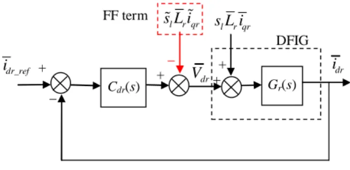
. (9)+ _ Gr(s) + Vdr+ dr_ref i idr l r qr s L i _ DFIG Cdr(s) l r qr s L i%% + FF term
Figure 2: Control bock of q-axis rotor current for grid synchronization
Take the d-axis rotor current control for instance. The control block is shown as Fig. 2, where Cdr(s)
represents a PI controller. The parameters of the PI controller can be derived by the internal model control (IMC) method as:
1
( )
( )
r r dr r sL
R
C
s
G
s
s
ω
s
α
α
α
−=
=
+
, (10)where α is a IMC design parameter. In the case of a first-order system, α is set to be the desired bandwidth of the closed-loop system. The relationship between the bandwidth and the rise time is α=ln9/trise, where triserepresents the rise time [4].
The term
s L i
l r qr can be considered as a disturbance. A disturbance estimation is exploited as a feed-forward term for compensation, as shown in the red box in Fig. 2. However, it is also possible to introduce an "active damping" factor to the control loop, so that the disturbance can be damped with the same time constant as the control dynamics [4].controller: CTω(s) + _ qr_ref i qr i qr v ref
ω
ω
e_ref T dr_ref i dr i ref Q vdr DFIG controller: CiT(s) controller: CiQ(s) controller: Cvi_qr(s) controller: Cvi_dr(s) + _ + _Figure 3: Decoupled speed (active power) and reactive power control of DFIG
3.2
Active power optimization control
As mentioned before, DFIG is controlled according to a predefined power-speed characteristics profile to optimize the wind power extraction. Thus, the active power optimization control is actually the speed control. According to decoupled d-q axis mapping, d- and q-axis rotor current components are controlled for reactive and active power respectively. Cascaded PI or IP controllers are used, and the IMC or pole placement method is used respectively to derive the parameters of the controllers.
Active power control comprises 3 cascaded loops:
q-axis rotor current control, torque control and speed
control, while the reactive power control comprises reactive power and d-axis rotor current control. A schematic diagram of the decoupled speed (active power) and reactive power control is shown in Fig. 3, where the controllers are either IP or PI regulators except for the torque control part. Considering that torque is difficult to be measured, it is most often controlled in an open-loop manner [4].
3.2.1 Current control
To derive decoupled rotor current control laws,
several conditions should be noted beforehand. From equation (1),
ψ
ds andψ
qs approximatelyequal
v
qsandv
dsrespectively in steady state. Thus,1 p.u.
0 p.u.
≈
=
≈
=
ds qs qs dsψ
v
ψ
v
. (11) Then, according to d,q-axis stator flux linkage formulations in equation (2):(
)
1
1
,
≈
−
≈ −
m ds m dr qs qr s sL
i
L i
i
i
L
L
. (12) Denote 2 1 m r sL
X = L
L
−
, and substitute the rotor flux linkage equation (2) and the stator-rotor current equation (12) into the rotor voltage equation (1), then, 1 qr r qr qr qr sX d
v = R i +
i + E
ω
dt
, (13) where 1
=
+
m qr l dr sL
E
s
X i
L
can be treated as a disturbance. Thus, the transfer function between therotor current and the rotor voltage is: 1
( )
1
( )
( )
qr vi_qr qr r sI
s
G
s
X
V
s
R
s
ω
=
=
+
. (14)Similar to that of the grid synchronization process, the parameters of the PI controller can be derived by the IMC method as:
1 1
( )
( )
r vi_qr qr sX
R
C
s
G
s
s
ω
s
α
α
α
−=
=
+
. (15)3.2.2 Torque control
Torque can be expressed in the form of controllable
q-axis rotor current by substituting equations (11-12)
into (3): m e qr s
L
T
i
L
= −
. (16) The transfer function between the q-axis rotor current and the torque then becomes( )
( )
( )
qr s iT e mi
s
L
C
s =
T s
= −
L
, (17)which is used for the open-loop torque control.
3.2.3 Speed control
The inertia of the rotating wind turbine system is very high. However, compared to the turbine itself and the generator rotor, the inertia of the shaft is negligibly small [10]. From the generator rotor point of view and neglecting the shaft inertia, the mechanical balance equation can then be derived as [11]:
2 T T r e g
T
J
d
T
J +
n
n
dt
ω
η
η
+ =
, (18)where TT is the turbine torque created by the
aerodynamic lift on the blades; Te is the generator
electromagnetic torque, id. est., the resisting torque; Jgis the inertia of the generator rotor itself; JT is the
inertia of the turbine; n is the gearbox reduction ratio;
η is the energy transmission efficiency; ωr is the
rotating speed of the generator rotor in mechanical measurement.
Normally, the wind turbine is a lot heavier than the generator, and JT/ηn
2
is larger than the generator rotor inertia [10]. Denote the equivalent inertia and the input torque by J and Tmrespectively, the above
equation can be rewritten as: r m e
d
T
T
J
dt
ω
+ =
, (19) Since the torque to speed loop is a pure integral element, an IP regulator is used for the speed control to derive a second-order form for the closed-loopsystem, as shown in Fig. 4. Considering that current dynamics are much faster than speed dynamics, the electromagnetic torque Tecan be expressed as Te_ref.
+ _ Ki/s 1/(Js) + Te_ref+ ref
ω
Kp + _ mT
rω
Figure 4: Control block of the speed
The transfer function of the closed loop system turns to be a standard second-order form as:
2
( )
( )
(
)
i r ref p iK /J
s
=
s
s + K /J s + K /J
ω
ω
. (20)The parameters of the controller are then tuned through pole placement. Denote the damping factor and the natural frequency of the second order system by
ζ
d and ωnd respectively, and theparameters of the IP controller can then be given by:
2
2
p d nd i ndK =
J
K =
J
ζ ω
ω
. (21)There are some approximation methods on evaluating the relationship between the settling time tsd and ζd and ωnd. In a particular situation of an
over-damped system, ωnd ≈5.8/tsd [3]. Once the
desired dynamic response is evaluated, the IP controller parameters can then be tuned accordingly. Let's recall that the synchronization process is very fast, usually less than 100ms, and once it is accomplished, right after the power control process starts. Considering that the inertia of a wind turbine is very high, the speed is almost constant during the synchronization. Therefore, the initial value of the integral term of the IP controller can be accordingly set as ωst·Kp/Ki , where ωst stands for the predefined
initial speed of the synchronization.
3.3 Reactive power control
As mentioned above, the converter GSC is controlled to operate with unity power factor. This means that the transmission of reactive power between DFIG and the grid is only through the stator [9]. The reactive power at the grid terminals is then equal to the stator reactive power:
s qs ds ds qs
Q
=
Q
=
v i
−
v i
, (22) Likewise, substitute equations (5) and (12) into (22) and the expression can be derived in the form of controllable d-axis rotor current as:1
(1
)
=
−
m dr sQ
L i
L
. (23) Then,(
)
1
1
−
dr s mi =
L Q
L
. (24) Particularly, when the desired stator reactive power is zero, then1
dr mi =
L
. (25) The current control in the reactive control loop is similar to that of the speed (active power) control loop, and will not be reiterated here.4 Strongly coupled approach and
modelling methods on Samcef
4.1 Strongly coupled approach
A coupled mechatronic problem can be modularly decomposed into a mechanical system and a control system. The mechanical system can be modelled using the finite element flexible multibody formalism, and the control system is usually described using block diagram language. To solve the coupled problem, numerical time integration methods have to be applied for both subsystems. In the case of a weak coupling approach, respective integration solvers are used for the subsystems accordingly. The coupling of the subsystems then implies the coupling of the different solvers, so that stability and convergence properties can be affected [5]. For the case of a strongly-coupled approach, only one optimized solver is applied to both subsystems so that the required order of accuracy and stability can be easily ensured for the simulation of a mechatronic system.
In flexible multibody dynamics, the Newmark family of implicit solvers have been applied extensively. To extend the solver to represent a mechatronic system, an extended generalized-α method is proposed in reference [6]. Based on that, an integrated solver has newly been developed into Samcef for the simulation of flexible multibody structures coupled with non-mechanical subsystems. The formulation relies on a modular block diagram description of the control system, which is now available on Samcef.
Mechanism
Control system
y
( , , , )
q q q
& &&
λ
Figure 5: Schematic diagram of the coupling in a mechatronic system
Based on the finite element method for the mechanical part and on the block diagram language for the control part, a mechatronic system can be described as shown in Fig. 5, where q is the vector of mechanical coordinates,λis the vector of Lagrange multipliers related with the kinematic constraints and y is the vector of control outputs. The dynamics can be represented by the following coupled equations:
q
Mq
Φ ( λ
Φ) g(q, q, ) L y
0
Φ(q)
0
x
f (q, q, q,λ, x, y, )
0
y h(q, q, q,λ, x, y, )
0
T ak
p
t
k
t
t
+
+
−
−
=
=
−
=
−
=
&&
&
& &&
&
& &&
, (26)where the first two equations are the equations of motion of the mechanical subsystem and the last two equations are the state space equations of the control subsystem. La is the output localization matrix, the term Lay represents the generalized forces exerted by the actuators and generators on the mechanical system, x is the vector of control state variables and the other symbols are commonly known and can be referred to [6]. The strongly coupled mechanical and state equations are obtained by numerical assembly and their time-domain simulation is based on an extension of the generalized-α method. A detailed description of the time integration algorithm can be found in [6].
4.2 Modular modelling of DFIG control
systems on Samcef
With the integration of the new strongly-coupled solver, the DFIG control system were modelled for S4WT. The system is decomposed into subsystems and modularized. Decomposition is based on the analysis of the function of each component. All models, including the generator itself and the controllers, are aimed at general-purpose use. Extra nodes are introduced to represent the state and output variables from the generating control system, which is similar to the way for the structure system. A tangent matrix can then be derived for the Newton iteration, with difference in the coefficients for state variables and structural nodes.
5 Simulation and validation
In this section, two simulation examples will be presented for validating the models of the DFIG control system and also the strongly-coupled solver. A 2MW DFIG prototype model is used for the simulation analysis. The parameters of the DFIG are listed as follows [7]:
Base voltage (line-to-line): Vbase= 690 V;
Base power: Pbase= 2 MW;
Grid frequency: fs= 50 Hz;
Number of poles: np= 4;
Stator resistance: Rs= 0.00488 p.u.;
Rotor resistance : Rr= 0.00549p.u.;
Stator Leakage inductance: Lsl= 0.09241 p.u.;
Rotor leakage inductance: Lrl= 0.09955 p.u.;
Mutual inductance: Lm= 3.95279 p.u..
The inertia of the generator itself is 100kg·m2. However, since the inertia of the wind turbine system is barely known, several estimation methods are discussed in reference [12]. Usually, the inertia time constant of a 2MW wind turbine ranges from 3.5s to 6s.
For the per-unit representation, here in this paper, the base current is defined as Ibase=Pbase/Vbase; the
base resistance Rbase= Vbase/Ibase = ωsLbase, where Lbase
is the base inductance; the base flux linkage
ψbase=Vbase/ωs; the base speed ωbase=2ωs/np; and
consequently the base torque Tbase=Pbase/ωbase.
5.1 DFIG alone with defined torque input
In this section, a simple example of the DFIG running alone with defined driving torque is studied. The purpose of this simulation example is to verify the model and the control strategies. The DFIG is operating given 1p.u. driving torque in the verybeginning. When the speed reaches 0.8p.u. of the base speed, the synchronization process starts. Once this process is completed, then right away starts the speed and reactive power control. Initially, the reference speed is set to be 1p.u.. Then after 4s, it is changed to 0.9p.u., and again, it is changed to 1.1p.u. from 6s. Finally, while maintaining the same reference speed, the driving torque is ramped down to 0.5p.u. from 8.5s to 9.5s.
As for the parameters of the controller, since the dynamics of the electrical system is much faster than the mechanical system, the rise time for the current control loop is set to 10ms (α = 219 for the PI controllers), while the settling time for the speed control loop is set to 1s (ζd =1, ωnd=5.8 for the IP
controllers). For the integrated FEM solver, an automatic time step scheme is used for the simulation.
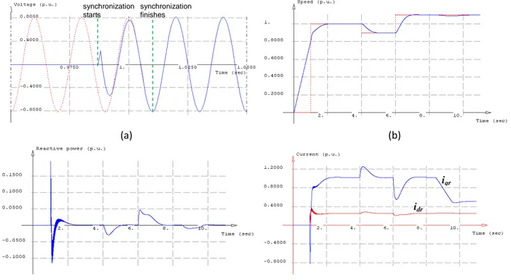
Selected simulation results are shown in Fig. 6. Fig.6(a) shows the grid synchronization process of the A-phase stator voltage with the A-phase grid voltage. This process takes only about 25ms. As one can see from Fig.6(b) and Fig.6(c), the response for both speed and reactive power control are satisfactory. From Fig.6(d), it can be easily derived that speed control is determined by the control of
q-axis rotor current and reactive power control is by
the d-axis rotor current, and thus they are decoupled.
(a) (b)
(c) (d)
Figure 6: DFIG alone: (a) Grid synchronization response; (b) Speed response; (c) Stator reactive power; (d) q,d-axis rotor current.
iqr idr synchronization starts synchronization finishes
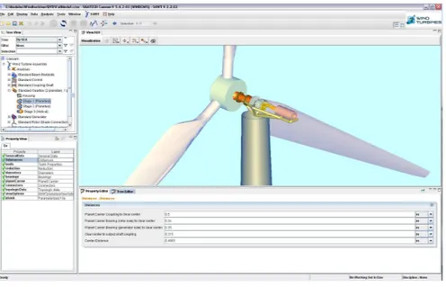
Figure 7: A model of wind turbine generating systems on S4WT
(a) (b)
(c) (d)
Figure 8: Full wind turbine response: (a) Grid synchronization process; (b) Speed response with different wind speeds; (c) Power output; (d) q,d-axis rotor current.
5.2 The integration of the wind turbine
structure model with the DFIG model
A systematic model of a 2MW wind turbine integrated with the DFIG model is presented in this section. The model on S4WT is shown in Fig. 7. Some selected parameters of the turbine system are as: 41m of blade length, 75m of tower height and 106 of the gearbox ratio. The blades are modeled as elastic beams and the aerodynamic loads are computed using the blade element momentum theory, see [13] for more details about the underlyingformulation. The interest here is to analyze the control-generator-structure interactions in a wind turbine system.
An approximate inertia time constant 3.5s is used for deriving the IP controller parameters. However, since it's difficult to be accurate, a higher damping factor could be used for the second-order system of the closed speed control loop. Given that the inertia of the turbine system is very large, the settling time is set as 2.5s. As for the PI controllers, the same parameters are used as those in the previous
11m/s 8m/s Activepower Reactive power Turbine speed P o w e r iqr idr synchronization starts synchronization finishes
example.
The simulation situation is as follows. The initial wind speed is set to 8m/s and the initial turbine speed is to be 1.1rad/s (accordingly 0.74p.u.). The aerodynamic torque drives the turbine to rotate. Grid synchronization control starts when the generator rotating speed reaches 0.8p.u.. After 8s, the wind speed changes to 11m/s. For 8m/s of the wind speed, the maximum wind power is assumed to be extracted with 0.9p.u. of the rotating speed, while 1.1p.u. is that for a wind speed of 11m/s. A wind power-speed characteristic diagram is shown on the bottom right of Fig. 8(b). Also, an automatic time step scheme is applied. Selected simulation results are shown in Fig. 8.
6 Conclusions
This paper studies the modelling and control of DFIG in variable-speed wind turbine systems based on an integrated, strongly-coupled finite element approach. New block diagram functionalities for the description of control systems are integrated into Samcef/Mecano multibody dynamics solver. This allows the simulation of mechatronic systems in a strongly-coupled way, so that the intricacy and uncertainty of using a third-party control engineering software can be avoided. The DFIG generator and the controller models are developed in a modular, parameterized way. They are built to expand the MECANO wind turbine package, and are also aimed at general-purpose use based upon strongly-coupled simulation. Detailed control strategies are presented for grid synchronization and power optimization. Simulation results show the validity of the DFIG model and the strongly-coupled simulation approach. A comprehensive wind turbine system model is presented to analyze the coupling effects among different components. Control of the generator will influence both the energy extraction and the mechanical structure life due to the mutual coupling.
Acknowledgements
This research work was carried out under grant number 850533 (DYNAWIND) from the Walloon Region (Belgium) which is gratefully acknowledged.
References
[1]. Géradin, M. and Cardona, A., Flexible multibody
dynamics: a finite element approach, John Wiley
& Sons, New York, 2001.
[2]. Chowdhury, B. H. and Chellapilla, S., "Double-fed induction generator control for variable speed wind power generation", Electric
Power Systems Research, 2006, 76, 786-800.
[3]. Tapia, G. Santamaria, G. Telleria, M. and
Susperregui, A., "Methodology for smooth connection of doubly fed induction generators to the grid", IEEE Transactions on Energy
Conversion, 2009, 24, 959-971
[4]. Petersson, A., Analysis, modeling and control of
Doubly-Fed Induction Generators for wind turbines, PhD thesis, Chalmers University of
Technology, Göteborg, Sweden, 2005.
[5]. Busch, M. and Schweizer, B., "Numerical Stability and Accuracy of Different Co-Simulation Techniques: Analytical Investigations Based on a 2-DOF Test Model", Proceedings of the 1st Joint
International Conference on Multibody system Dynamics, Lappeenranta, Finland, May 25-27,
2010.
[6]. Brüls, O. and Golinval, J. C., "The generalized-α
method in mechatronic applications", Zeitschrift
für angewandte mathematik und mechanik
(ZAMM), 2006, 86, 748-758.
[7]. Ekanayake, J. B., Holdsworth, L. and Jenkins N., "Comparison of 5th order and 3rd order machine models for doubly fed induction generator (DFIG) wind turbines", Electric Power Systems Research, 2003, 67, 207-215.
[8]. Gomez, S. A. and Amenedo, J. L. R., "Grid synchronisation of doubly fed induction generators using direct torque control",
Proceedings of IEEE 28th Annual conference of the Industrial Electronics Society, Sevilla, Spain,
Nov. 5-8, 2002.
[9]. Hansen, A. D., Sørensen, P., Iov, F. and Blaabjerg, F., "Centralised power control of wind farm with doubly fed induction generators",
Renewable Energy, 2006, 31, 935-951.
[10]. Rostoen, H. O., Undeland, T. M. and Gjengedal T., "Doubly fed induction generator in a wind turbine", Proceedings of the IEEE/Cigre workshop on wind power and the impacts on power systems, Oslo, Norway, Jun. 17-18, 2002.
[11]. Cetinkunt, S., Mechatronics, John Wiley & Sons, Inc., Hoboken, New Jersey, 2007.
[12]. Rodriguez, A. G. G., Improvement of a
fixed-speed wind turbine soft-starter based on a sliding-mode controller, PhD thesis, University of
Seville, Seville, Spain, 2006.
[13]. Heege, A., Betran, J. and Radovcic, Y., "Fatigue load computation of wind turbine gearboxes by coupled finite element, multi-body system and aerodynamic analysis", Wind Energy, 2007, 10, 395–413.