HAL Id: hal-00444087
https://hal.archives-ouvertes.fr/hal-00444087v2
Preprint submitted on 19 Jan 2010
HAL is a multi-disciplinary open access
archive for the deposit and dissemination of
sci-entific research documents, whether they are
pub-lished or not. The documents may come from
teaching and research institutions in France or
abroad, or from public or private research centers.
L’archive ouverte pluridisciplinaire HAL, est
destinée au dépôt et à la diffusion de documents
scientifiques de niveau recherche, publiés ou non,
émanant des établissements d’enseignement et de
recherche français ou étrangers, des laboratoires
publics ou privés.
model dependencies between genetic markers
Raphaël Mourad, Christine Sinoquet, Philippe Leray
To cite this version:
Raphaël Mourad, Christine Sinoquet, Philippe Leray. Learning a forest of Hierarchical Bayesian
Networks to model dependencies between genetic markers. 2010. �hal-00444087v2�
L
ABORATOIRE D’I
NFORMATIQUE DEN
ANTES-A
TLANTIQUE— KnOwledge and Decision (KOD) —
R
ESEARCH
R
EPORT
No hal-00444087
January 2010
Learning a forest of Hierarchical Bayesian
Networks to model dependencies between genetic
markers
Rapha¨el Mourad
†, Christine Sinoquet‡, Philippe Leray†
†LINA, UMR CNRS 6241, Ecole Polytechnique de l’Universit´e de Nantes, rue Christian Pauc, BP 50609, 44306 Nantes Cedex 3, France,
‡LINA, UMR CNRS 6241, Universit´e de Nantes, 2 rue de la Houssini`ere, BP 92208, 44322 Nantes Cedex, France
LINA, Université de Nantes – 2, rue de la Houssinière – BP 92208 – 44322 NANTES CEDEX 3
Tél. : 02 51 12 58 00 – Fax. : 02 51 12 58 12 – http
:
//www.sciences.univ-nantes.fr/lina/
Learning a forest of Hierarchical Bayesian
Net-works to model dependencies between genetic
mark-ers
26p.
Les rapports de recherche du Laboratoire d’Informatique de Nantes-Atlantique sont disponibles aux formats PostScript®et PDF®`a l’URL :
http://www.sciences.univ-nantes.fr/lina/Vie/RR/rapports.html
Research reports from the Laboratoire d’Informatique de Nantes-Atlantique are available in PostScript®and PDF®formats at the URL:
http://www.sciences.univ-nantes.fr/lina/Vie/RR/rapports.html
© January 2010 by
Rapha¨el Mourad
†, Christine Sinoquet‡, Philippe
Learning a forest of Hierarchical Bayesian
Networks to model dependencies between
genetic markers
Rapha¨el Mourad
†, Christine Sinoquet‡, Philippe Leray†
raphael.mourad,christine.sinoquet,philippe.leray@univ-nantes.fr
Abstract
We propose a novel probabilistic graphical model dedicated to represent the statistical dependencies between genetic markers, in the Human genome. Our proposal relies on building a forest of hierarchical latent class models. It is able to account for both local and higher-order dependencies between markers. Our motivation is to reduce the dimension of the data to be further submitted to statistical association tests with respect to diseased/non diseased status. A generic algorithm, CFHLC, has been designed to tackle the learning of both forest structure and probability distributions. A first implementation of CFHLC has been shown to be tractable on benchmarks describing 105 variables for 2000 individuals.
1
Introduction
Genetic markers such as SNPs are the key to dissecting the genetic susceptibility of complex diseases: they are used for the purpose of identifying combinations of genetic determinants which should accumu-late among affected subjects. Generally, in such combinations, each genetic variant only exerts a modest impact on the observed phenotype, the interaction between genetic variants and possibly environmental factors being determining in contrast. Decreasing genotyping costs now enable the generation of hun-dreds of thousands of genetic variants, or SNPs, spanning whole Human genome, accross cohorts of cases and controls. This scaling up to genome-wide association studies (GWAS) makes the analysis of high-dimensional data a hot topic. Yet, the search for associations between single SNPs and the variable describing case/control status requires carrying out a large number of statistical tests. Since SNP patterns, rather than single SNPs, are likely to be determining for complex diseases, a high rate of false positives as well as a perceptible statistical power decrease, not to speak of untractability, are severe issues to be overcome.
The simplest type of genetic polymorphism, Single Nucleotide Polymorphism (SNP), involves only one nucleotide change, which occurred generations ago within the DNA sequence. To fix ideas, we emphasize that one single individual can be uniquely defined by only30 to 80 independent SNPs and unrelated individuals differ in about0.1% of their 3.2 billion nucleotides. Compared with other kinds of
DNAmarkers, SNPs are appealing because they are abundant, genetically stable and amenable to high-throughput automated analysis. Consistently, advances in high-high-throughput SNP genotyping technologies lead the way to various down-stream analyses, including GWASs.
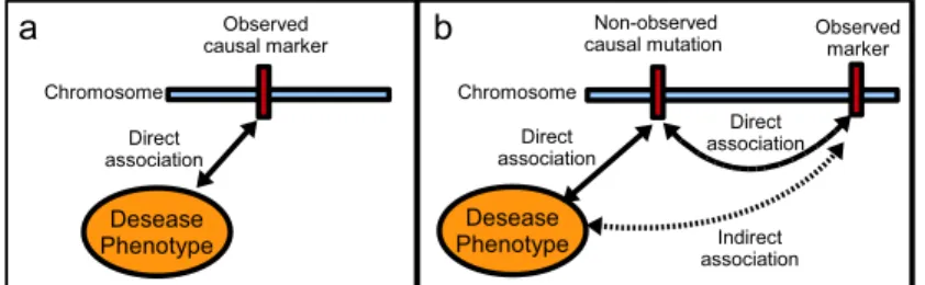
Exploiting the existence of statistical dependencies between SNPs, also called linkage disequilibrium (LD), is the key to association studies achievement (Balding (2006)). Indeed, a causal variant may not be a SNP. For instance, insertions, deletions, inversions and copy-number polymorphisms may be causative of disease susceptibility. Nevertheless, a well-designed study will have a good chance of including one or more SNPs that are in strong LD with a common causal variant. In the latter case, indirect association with the phenotype, say affected/unaffected status, will be revealed (see Figure1).
Figure 1: a) Direct association between a genetic marker and the phenotype. b) Indirect association between a genetic marker and the phenotype.
Interestingly, LD is also the key to reduce data dimensionality in GWASs. In eukaryotic genomes, LD is highly structured into the so-called ”haplotype block structure” (Patit et al. (2001)): regions where correlation between markers is high alternate with shorter regions characterized by low correlation (see Figure2). Relying on this feature, various approaches were proposed to achieve data dimensionality reduction: testing association with haplotypes (i.e. inferred data underlying genotypic data) (Schaid (2004)), partitioning the genome according to spatial correlation (Pattaro et al. (2008)), selecting SNPs informative about their context, or SNP tags (Han et al. (2008)) (for other references, see Liang et al.
(2008) for example). Unfortunately, these methods do not take into account all existing dependencies since they miss higher-order dependencies.
Figure 2: LD plot (matrix of pairwise dependencies between genetic markers or linkage disequilibrium). Human genome, chromosome2, region [234 357kb - 234 457kb]. For a pair of SNPs, the colour shade is all the darker as the correlation between the two SNPs is high.
Probabilistic graphical models offer an adapted framework for a fine modelling of dependencies be-tween SNPs. Various models have been used for this peculiar purpose, mainly Markov fields (Verzilli
et al. (2006)) and Bayesian networks (BNs), with the use of hierarchical latent BNs (embedded BNs
(Nefian (2006)); two-layer BNs with multiple latent (hidden) variables (Zhang and Ji (2009)). Although modelling SNP dependencies through hierarchical BNs is undoubtedly an attractive lead, there is still room for improvement. Notably, scalability remains a crucial issue.
In this paper, we propose to use a forest of Hierarchical Latent Class models (HLCMs) to reduce the dimension of the data to be further submitted to association tests. Basically, latent variables capture the information born by underlying markers. To their turn, latent variables are clustered into groups and, if relevant, such groups are subsequently subsumed by additional latent variables. Iterating this process yields a hierarchical structure. First, the great advantage to GWASs is that further association tests will be chiefly performed on latent variables. Thus, a reduced number of variables will be examined. Second, the hierarchical structure is meant to efficiently conduct refined association testing: zooming in through narrower and narrower regions in search for stronger association with the disease ends pointing out the potential markers of interest.
However, most algorithms dedicated to HLCM learning fail the scalability criterion when data de-scribe thousands of variables and a few hundreds of individuals. The contribution of this paper is twofold: (i) the modelling of dependencies between clusters of SNPs, (ii) the design of a tractable al-gorithm, CFHLC, fitted to learn a forest of HLCMs from spacially-dependent variables. In the line of a hierarchy-based proposal of Hwang and collaborators (Hwang et al. 2006), our method yet implements data subsumption, meeting two additional requirements: (i) more flexible thus more faithful modelling of underlying reality, (ii) control of information decay due to subsumption. Section 2 motivates the design of HLCMs. Section 3 points out the few anterior works devoted to HLCM learning. Then, after an unfor-mal description of the FHLC model, Section 4 focuses on the general outline of the method proposed for FHLCM learning. In Section 5, we give the sketch of algorithm CFHLC. Section 6 presents experimental results and discusses them.
7
2
Motivation for HLC modelling
From now on, we will restrain to discrete variables (either observed or latent).
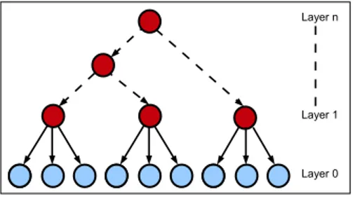
A Latent Class Model (LCM) is defined as containing a unique latent variable connected to each of the observed variables. The latent variable influences all observed variables simultaneously and hence renders them dependent. In the LCM framework, an underlying assumption states that the observed vari-ables are pairwise independent, conditional on the latent variable (Zhang (2004)). Since each state of the latent variable corresponds to a class of individuals, this assumption, also called local independence (LI), can be restated as pairwise independency, conditional on latent class membership. The intuition behind LI is that the latent variable is the only reason for the dependencies between observed variables. However, this assumption is often violated for observed data. To tackle this issue, HLCMs were proposed as a generalization of LCMs. HLCMs are tree-shaped BNs where leaf nodes are observed while internal nodes are not. In a Bayesian network, local dependency between variables may be modelled through the use of an additional latent variable (see Figure3). At a larger scale, multiple latent variables organized in a hierarchical structure allow high modelling flexibility. Figure4illustrates the ability of HLCMs to depict a large variety of relations encompassing local to higher-order dependencies.
Figure 3: (a) Latent Bayesian network modelling a local dependency between B and C nodes. (b) Mod-elling of the local dependency between B and C nodes through a latent hierarchical model.
Figure 4: Hierarchical latent lodel. The light shade indicates the observed variables whereas the dark shade points out the latent variables.
3
Background for HLC model learning
Various methods have been conceived to tackle HLCM learning. These approaches differ by the follow-ing points: (i) structure learnfollow-ing; (ii) determination of the latent variables’ cardinalities; (iii) learnfollow-ing of parameters, i.e. unconditional and conditional probabilities; (iv) scalability; (v) main usage.
As for general BNs, besides learning of parameters (θ), i.e. unconditional and conditional probabil-ities, one of the tasks in HLCM learning is structure (S) inference. The HLCM learning methods fall into one of two categories. The first category, structural Expectation Maximization (SEM), successively optimizes θ | S and S | θ. Amongst few proposals, hill-climbing guided by a scoring function was designed (Zhang (2003)): the HLCM space is visited through addition or removal of latent nodes alter-nating with addition or dismissing of states for existing nodes. Other authors adapted a SEM algorithm combined with simulated annealing to learn a two-layer BN with multiple latent variables (Zhang and Ji (2009)). Alternative approaches implement ascending hierarchical clustering (AHC). Relying on pair-wise correlation strength, Wang and co-workers first build a binary tree; then they apply regularization and simplification transformations which may result in subsuming more than two nodes through a latent variable (Wang et al. (2008)). Hwang and co-workers’ approach confines the HLCM search space to binary trees augmented with possible connections between siblings (nodes sharing the same parent into immediate upper layer) (Hwang et al. (2006)). Moreover, they constrain latent variables’ arity to binarity. However, the latter approach is the only one we are aware of that succeeds in processing high-dimensional data: in an application dealing with a microarray dataset, more than6000 genes have been processed for around60 samples. To our knowledge, no running time was reported for this study.
Nevertheless, the twofold binarity restriction and the lack of control for information decay as the level increases are severe drawbacks to achieve realistic SNP dependency modelling and subsequent associa-tion study with sufficient power.
4
Constructing the FHLC model
4.1
The FHLC model
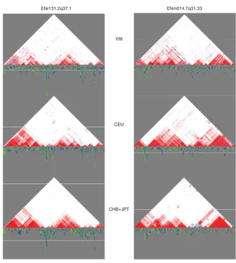
The HLCMs offer several advantages for GWASs. Beside data dimensionality reduction, they allow a simple test of direct dependency beween an observed variable and a target variable such as the pheno-type, conditional on the latent variable, parent of the observed variable. Note that the phenotype variable is not included in the HLCM. In the context of GWASs, this test helps finding the markers which are directly associated with the phenotype, i.e. causal markers, should there be any. Second, the hierarchical structure allows zooming in through narrower and narrower regions in search for stronger association with the disease. This zooming process ends pointing out the potential markers of interest. Thirdly, the latent variables may be interpreted in a biological meaning. For instance, in the case of haplotypes, that is, phased genotypes, the latent variables are likely to represent the so-called haploblock structure of LD. However, SNP dependencies would rather be more wisely modelled through a Forest of HLCMs (FHLCM), best accounting for possible higher-order dependencies on the genome. Indeed, in the case of a forest, higher-order dependencies are captured only when relevant, i.e when meeting a strength cri-terion. Also, not the least advantage over the HLC model lies in that variables are not constrained to be dependent upon one another, either directly or indirectly. Therefore, FHLCMs allow to model a larger set of configurations than HLCMs do. Typically, an HLCM is limited to manage LD structure modelling where clusters of close SNPs are dependent whereas no dependency exists between groups of distant SNPs or SNPs located on different chromosomes. But realistic modelling requires a more flexible frame-work. For instance, the six LD plots shown in Figure5give the intuition of the local dependency while also illustrating various cases of inter-dependency between clusters of SNPs.
An FHLCM consists of a Directed Acyclic Graph (DAG), also called the structure, whose non-connected components are trees, and ofθ, the parameters (further defined). Figure6illustrates a possible
9
Figure 5: LD plot (matrix of LD measures for each pair of SNPs) in regions Encode ENr131.2q37.1 and ENm014.7q31.33 for the three populations YRI, CEU and CHB+JPT of the HapMap project (http://hapmap.ncbi.nlm.nih.gov/). The darker the shade, the stronger the LD.
structure for an FHLCM.
Figure 6: A forest of hierarchical latent models. This forest consists of two trees, of respective heights2 and3.
4.2
Principle
Our method takes as an input a matrixDXdefined on a finite discrete domain, say{0, 1, 2} for SNPs,
describingn individuals through p variables (X = X1, ..., Xp). Algorithm CFHLC yields an FHLCM,
that is a forest structure andθ, the parameters of a set of a priori distributions and local conditional distributions allowing the definition of the joint probability distribution. Two search spaces are explored: the space of directed forests and the probability space. In addition, the whole set of latent variablesH of
the FHLCM is output, together with the associated imputed data matrix.
To handle high-dimensional data, our proposal combines two strategies. The first strategy splits up the genome-scale data into contiguous regions. In our case, splitting into (large) windows is not a mere implementational trick; it meets biological grounds: the overwhelming majority of dependencies between genetic markers (including higher-order dependencies) is observed for close SNPs. Then, an FHLCM is learnt for each window in turn. Within a window, subsumption is performed through an adapted AHC procedure: (i) at each agglomerative step, a partitioning method is used to identify clusters of variables; (ii) each such cluster is intended to be subsumed into an latent variable, through an LCM. For each LCM, parameter learning and missing data imputation (for the latent variable) are performed.
4.3
Node partitioning
Following Martin and VanLehn (1995), ideally, we would propose to associate a latent variable with any clique of variables in the undirected graph of dependency relations exhibiting pairwise dependencies of strengths being above a given threshold (see Figure7). However, searching for such cliques is an NP-hard task. Moreover, in contrast with the previous authors’ objective, FHLCMs do not allow clusters to have more than one parent each: non-overlapping clusters are required for our purpose. Thus, an approxi-mate method solving a partitioning problem when provided pairwise dependency measures must be used.
Figure 7: (a) Three pairwise dependent variables (clique). (b) Latent model: the three variables depend on a common latent variable. The dark shade indicates the latent variable designed to model the pairwise dependency between the three variables.
4.4
Parameter learning and imputation
A steep task is choosing - ideally optimizing - the cardinality of each LCM’s latent variable. Instead of using an arbitrary constant value common to all latent variables, we propose that the cardinality be adapted for each latent variable through a function of the underlying cluster’s size. The underlying ratio-nale for choosing this function is the following: the more child nodes a latent variable has, the larger is the number of latent class value assignments for the child nodes. Therefore, the cardinality of this latent variable should depend on the number of child nodes. Nonetheless, to keep the model complexity within reasonable limits, a maximal cardinality is fixed.
Parameter learning is carried out step by step, each time generating additional latent variables and imputing their values for each individual. Atithstep, this task simply amounts to performing parameter
learning for as many LC models as there are clusters of variables identified. We recall that the nodes in the topology of an LCM reduce to a root and leaves. Therefore, atithstep, each LCM’s structure is rooted in
a newly created latent variable. When latent variables are only source nodes in a BN, parameter learning may be performed through a standard EM procedure. This procedure takes as an input the cardinalities of the latent variables and yields the probability distributions: prior distributions for those nodes with no
11
parents and distributions conditional to parents for the remaining nodes. After imputing the missing data corresponding to latent variables, new data are available to seed next step of the FHLCM construction: latent variables identified through stepi will be considered as observed variables during step i + 1.
It has to be noted that designing an imputation method to infer the values of the latent variable for each individual is in itself an investigation subject. Once the prior and conditional distributions have been esti-mated for a given LCM, probabilistic inference in BNs may be performed. A straightforward way would consist in imputing for each individual the latent variable value as follows: h∗ = argmax
h{p(H =
h/Xj1 = xj1, Xj2 = xj2, ..., Xjc = xjc)}. However, in the framework of probabilistic models, this
deterministic approach is disputable. In contrast, a more convincing alternative will draw a valueh for latent variableH, knowing the probabilities p(H = h/Xj1 = xj1, Xj2 = xj2, ..., Xjc = xjc) for each
individual.
4.5
Controlling information decay
In contrast with Hwang and co-workers’ approach, which mainly aims at data compression, information decay control is required: any latent variable candidateH in step i which does not bear sufficient in-formation about its child nodes must be unvalidated. As a consequence, such child nodes will be seen as isolated nodes in stepi + 1. The information criterion, C, relies on average mutual information I. It is scaled through entropyH: C = 1
sH
P
i ∈ cluster(H)
I(Xi,H)
min (H(Xi), H(H)), withsHthe size ofcluster(H).
5
Sketch of algorithm CFHLC
The user may tune various parameters: s, the window size, specifies the number of contiguous SNPs (i.e. variables) spanned per window;t is meant to constrain information dilution to a minimal threshold criterionC, described in Subsection4.5. Parametersa, b and cardmaxparticipate in the calculus of the
cardinality of each latent variable. Finally, parameter PartitioningAlg enables flexibility in the choice of the method devoted to cluster highly-correlated variables into non-overlapping groups.
Within each successive window, the AHC process is initiated from a first layer of univariate models. Each such univariate model is built for any observed variable in the setWi (lines4 to 6). The AHC
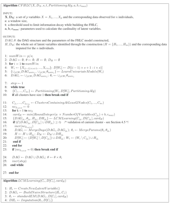
process stops if all clusters identified each reduce to a single node (line10) or if no cluster of size strictly greater than1 could be validated (line 23). Each cluster of at least two nodes is subject to LCM learning followed by validation (line13 to 22). In order to simplify the FHLCM learning, the cardinality of the latent variable is estimated as an affine function of the number of variables in the corresponding cluster (line14). Algorithm LCMLearning is plugged into this generic framework (line 15). After validation through thresholdt (lines 16 and 17), the LCM is used to enrich the FHLCM associated with current window (line18): (i) a specific merging process links the additional node corresponding to the latent variable to its child nodes; (ii) the prior distributions of the child nodes are replaced with distributions conditional to the latent variable. InWi, clusters of variables are replaced with the corresponding latent
variables; data matrixD[Wi] is updated accordingly (lines 19 and 20). In contrast, the nodes in
unvali-dated clusters are kept isolated for the next step. At last, the collection of forests, DAG, is successively augmented with each forest built within a window (line24). In parallel, due to assumed independency between windows, the joint distribution of the final FHLCM is merely computed as the product of the distributions associated with windows (line24).
AlgorithmCF HLC(X, DX, s, t, P artitioningAlg, a, b, cmax)
INPUT:
X, DX: a set ofp variables X = X1, ..., Xpand the corresponding data observed forn individuals,
s: a window size,
t: a threshold used to limit information decay while building the FHLC, a, b, cmax: parameters used to calculate the cardinality of latent variables.
OUTPUT:
DAG, θ: the DAG structure and the parameters of the FHLC model constructed,
H, DH: the whole set of latent variables identified through the construction(H = {H1, ..., Hm}) and the corresponding data
imputed for then individuals. 1: numW in ← p/s;
2: DAG ← ∅; θ ← ∅; H ← ∅; DH← ∅
3: fori = 1 to numW in
4: Wi← {X(i−1)×s+1, ..., Xi×s}; D[Wi] ← D[(i − 1) × s + 1 : i × s)]
5: {∪j∈WiDAGunivj, ∪j∈Wiθunivj} ← LearnU nivariateM odels(Wi)
6: DAGi← ∪j∈WiDAGunivj; θi← ∪j∈Wiθunivj 7: step ← 1
8: while true
9: {C1, ..., Cnc} ← P artitioning(Wi, D[Wi], P artitioningAlg)
10: if all clusters have size1 then break end if
11: Cj1, ..., Cjnc2← ClustersContainingAtLeast2N odes(C1, ..., Cnc) 12: nc2valid← 0
13: for k = 1 tonc2
14: cardH← min(RoundInteger(a × N umberOf V ariables(Cjk) + b, cmax) 15: {DAGjk, θjk, Hjk, DHjk} ← LCM Learning(Cjk, D[Cjk], cardH)
16: if(C(DAGjk, D[Cjk] ∪ DHjk) ≥ t) /* validation of current cluster - see Section 4.5 */ 17: incr(nc2valid)
18: DAGi← M ergeDags(DAGi, DAGjk); θi← M ergeP arams(θi, θjk) 19: H ← H ∪ Hjk; DH← DH∪ DHjk
20: D[Wi] ← (D[Wi] \ D[Cjk]) ∪ DHjk; Wi← (Wi\ Cjk) ∪ Hjk 21: end if
22: end for
23: if(nc2valid= 0) then break end if 24: DAG ← DAG ∪ DAGi; θ ← θ × θi
25: incr(step) 26: end while
27: end for
AlgorithmLCM Learning(Cr, D[Cr], cardH)
1: Hr← CreateN ewLatentV ariable()
2: DAGr← BuildN aiveStructure(Hr, Cr)
3: θr← standardEM (DAGr, D[Cr], cardH)
4: DHr← Imputation(θr, D[Cr])
Table 1: Sketch of algorithm CFHLC.
6
Experimental results and discussion
Algorithm CFHLC has been implemented in C++, relying on the ProBT library dedicated to BNs (http:// bayesian-programming.org). We have plugged into CFHLC a partitioning method, CAST, designed by Ben-Dor and co-authors (1999). CAST is a clique partitioning algorithm originally developped for gene expression clustering. As an input, it requires a similarity matrix and a similarity cutofft. The algorithm contructs the clusters one at a time. The authors define the affinitya(x) of an element x to be the sum
13
of similarity values betweenx and the elements present in the current cluster Copen. x is an element of
high affinity ifa(x) ≥ t|Copen|. Otherwise, x is an element of low affinity. To summarize, the algorithm
alternates between adding high affinity elements toCopenand removing low affinity elements from it.
When the process stabilizes,Copenis closed. A new cluster can be started.
We have generated simulated genotypic data using software HAPSIMU (http://l.web .umkc.edu/ liu-jian/). The default values for HAPSIMU parameters have been kept. They are recapitulated in Table2.
disease model parameters
disease prevalence 0.01
genotype relative risk 1.5
frequency of disease susceptible allele min:0.1, max: 0.3
population structure model parameters
proportion of YRI in cases 0.4
proportion of YRI in controls 0.6
number of generations 5
frequency difference min:0.1, max: 0.3
simulation parameters
sample size (number of individuals) 2000 proportion of cases in total sample 0.5
simulating times 1
genotype missing rate 0
Table 2: Parameter value adjustment for the generation of simulated genotypic data through software HAPSIMU.
CFHLC was run on a standard PC (3.8 GHz, RAM 3.3 Go). Three sample sizes were chosen to evaluate the scalability with respect to the number of observed variables:1k, 10k and 100k (In all cases, the number of individuals is set to2000). For the first round of experimentations, a rough adjustment of the CFHLC parameters has been performed. Hereafter, the default setting for CFHLC parameters is the following:a = 0.2, b = 2, cmax= 20, t = 0.5. On the following figures, boxplots have been produced
from20 benchmarks (exceptionally 5 in the 100k case of Figure8).
6.1
Temporal complexity
In the hardest case (100k), Figure8shows that only15 hours are required with a window size s set to 100. The previous figure highlights very low variances, indicated through boxplots. For the same dataset processed in the cases “s = 200” and “s = 600”, running times are 20.5 h and 62.5 h, respectively. For the same number of OVs (100k), Wang et al. report running times in the order of two months. Figure
9more thoroughly describes the influence of window size increase on running time. In the current ver-sion of CFHLC algorithm, successive windows are contiguous. For a given window size, the temporal complexity of CFHLC is expected to be linear with respect to the number of variables. However, on the basis of an execution time of20 mn for 1000 SNPs when s is set to 100, one would expect a running time of about33 h for 105SNPs. Following the same rationale, the expected running time for window
size200 should be around 42 h (in comparison to the observed execution time of 20.5 h). For window size600, the expected running time to be compared to the observed running time of 62.5 h is 92 h. The corresponding values for the ratio of observed running time to expected running time are the following ones:15 / 33 = 0.45 (s = 100); 20.5 / 42 = 0.49 (s = 200); 62.5 / 92 = 0.68 (s = 600). The existence of such ratios lead us to think that compression data may be drastic within many windows: the density of the dependency relations along the genome is heterogeneous.
1000
10000 100000
0
5
10
15
Number of SNPs
Runn
ing time (h)
s = 100, a = 0.2, b = 2, cmax = 20 and t = 0.5Figure 8: Running time versus number of variables. Low variances are highlighted through the boxplots drawn.
50
100 200 400 600
20
4
0
60
Window size
Runn
ing time (mn)
1000 SNPs, a = 0.2, b = 2, cmax = 20 and t = 0.5Figure 9: Impact of window size on running time.
6.2
Spacial complexity
We observe a dramatical decrease of the number of latent variables per layer (over the whole FHLCM) with the layer. Figure10exhibits this decrease in the case “s = 100”. A percentage of 64% of the latent variables are present in the first layer. In particular, the decrease between first and second layers amounts to60%. It has to be noted that although the number of latent variables is reduced, compared to Hwang and co-workers’ algorithm, additional memory allocation is requested to account for the distributions of the non binary latent variables. However, the datasets of size100k could be managed by our algorithm.
6.3
Impact of window size
Interestingly, Figure11highlights the decrease in the number of variables to be tested for association with the disease (from1000 observed variables to less than 200 forest roots in the case “s = 100”). In this case, algorithm CFHLC allows a reduction in the number of variables of more than80%.
15 1 2 3 4 5 6 7 0 50 10 0 Layer Number of LVs 150 1000 SNPs, s = 100, a = 0.2, b = 2, cmax = 20 and t = 0.5
Figure 10: Number of latent variables per layer over the whole FHLC model.
Like the number of latent variables, the number of layers increases with the window size, as shown in Figures12and13. This increase with window size is due to the fact that more higher-order interac-tions are taken into account. In average, around270 latent variables and 5 to 6 layers are reported for the case “s = 100”, whereas around 340 latent variables and 8 layers are identified for the case “s = 600”.
50 100 200 400 600 100 2 00 Window size Number of roots 1000 SNPs, a = 0.2, b = 2, cmax = 20 and t = 0.5
Figure 11: Impact of window size on the number of roots.
50 100 200 400 600 240 300 360 Window size Numer of LVs 1000 SNPs, a = 0.2, b = 2, cmax = 20 and t = 0.5
50 100 200 400 600 4 5 6 7 8 9 Window size Number of layers 1000 SNPs, a = 0.2, b = 2, cmax = 20 and t = 0.5
Figure 13: Impact of window size on the number of layers.
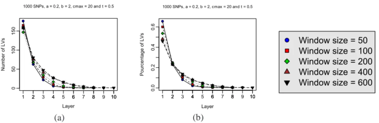
Figure14provides a more thorough insight of the distributions of latent variables between layers. Figure14(a) shows the impact of window size on the number of latent variables in a given layer while Figure 14(b) plots the ratios of the number of latent variables per layer to the total number of latent variables. Again, we observe a constant result: for all layers except the first one, the numbers (and ratios) are all the higher as the window size is larger. The exception relative to first layer is explained as follows: for a constant parameter setting of the partitioning algorithm, when the number of observed variables increases, that is when the window size increases, the number of clusters identified is smaller (with larger sizes). 2 4 6 8 10 0 50 1 00 150 Layer Number of LVs 1 2 3 4 5 6 7 8 9 10 1000 SNPs, a = 0.2, b = 2, cmax = 20 and t = 0.5 (a) 2 4 6 8 10 0.0 0.2 0.4 0.6 Layer Pourcentage of LVs 1 2 3 4 5 6 7 8 9 10 1000 SNPs, a = 0.2, b = 2, cmax = 20 and t = 0.5 (b) Window size = 50 Window size = 100 Window size = 200 Window size = 400 Window size = 600
Figure 14: (a) Average number of latent variables per layer over the whole FHLC model; impact of window size. (b) Average ratio of the number of latent variables per layer to the total number of latent variables; impact of window size.
6.4
Quality of the model
Figure15,16and17display how information fades while the layer number increases. Regarding window size600, the four first layers show average values around 0.62, 0.60, 0.59 and 0.58 for the scaled mutual information-based scoreC (see Figure15). In the highest layers, average scaled mutual information is at least equal to0.52 and 0.56 for the cases “s = 100” and “s = 600” respectively. Therefore, not only is a major point reached regarding tractability, information dilution is also controlled in an efficient way. The increasing variance is explained by the decreasing number of latent variables involved in the average calculation (see Figure10). In the highest layers, this sampling effect is all the more acute, entailing such
17
variations as that observed for layer8 and window size 50. In the latter case, a unique latent variable has been considered to compute the mean; it happened that the mutual information-based score calculated was outstandingly high in comparison with other values.
2 4 6 8 10 0.55 0.65 Layer Average sca led MI 1000 SNPs, a = 0.2, b = 2, cmax = 20 and t = 0.5 1 2 3 4 5 6 7 8 9
Window size = 50
Window size = 100
Window size = 200
Window size = 400
Window size = 600
Figure 15: Average scaled mutual information per layer over the whole FHLC model; impact of window size. 1 2 3 4 5 6 7 8 0.45 0.60 Layer Average sca led MI 1000 SNPs, s = 100, cmax = 20 and t = 0.5
a = 0.1 ß = 2
a = 0.2 ß = 2
a = 0.4 ß = 2
a = 0.2 ß = 4
a = 0.2 ß = 6
a = 0.1 b = 2
a = 0.2 b = 2
a = 0.4 b = 2
a = 0.2 b = 4
a = 0.2 b = 6
Figure 16: Average scaled mutual information per layer over the whole FHLC model; impact of parame-tersa and b.
As expected, average scaled mutual information raises with parametersa and b because latent vari-ables with larger cardinalities allow to capture more information about their child nodes, in the FHLCM (see Figure16). Besides, in the absence of information decay control, that is when thresholdt is set to 0, the average criterionC shows a particular trend: it first decreases throughout the first three layers then it increases while traversing fourth layer to highest layer (Figure17). Up to the third layer, a latent variable captures less and less information about its child nodes as the layer number rises: a loss of information is therefore observed. In contrast, latent variables in higher layers subsume but a few number of child nodes since clusters are smaller. Hence, these latent variables can easily provide sufficient information about their child variables. In addition, we observe that criterionC never goes down lower than 0.36. Expecting the constant conservation of more than a third of shared information between child and parent nodes was not foreseeable. Nonetheless, this observation advocates the importance of controlling information decay.
1 2 3 4 5 6 7 8 0.4 0.6 0.8 Layer Average sca led MI 1000 SNPs, s = 100, cmax = 20 and t = 0
Figure 17: Average scaled mutual information per layer over the whole FHLC model; absence of infor-mation decay control (t = 0).
A refined optimization of the adjustment of parametersa and b justifies in itself a thorough study and therefore lies beyond the scope of the present work. First, given a dataset, some investigations in wider ranges of values fora and b parameters must be performed: theoretically, the optimized values would ensure the lowest information dilution over the whole corresponding FHLCM constructed. In practice, for efficiency, a discretized search will have to be adapted.
Conversely, for a more refined analysis of the information decay through layers, we plan to run com-plementary tests on various datasets, under the same parameter setting ofa, b and t. Besides, Hwang and co-workers have published a figure similar to Figure15(Hwang et al (2006), Figure 3(a)), where the four first layers respectively exhibitC values around 0.65, 0.55, 0.52 and 0.51. Acknowledging the bias due to the differences in the datasets used by these authors and in our experimentations (see Figure
15), we observe similar orders of magnitude. In contrast to standard AHC, CFHLC allows flexible thus
early node clustering; therefore, if ever existing in the binary model and the FHLCM, the latent variable
subsuming a given cluster of nodes should be harboured at a lower level in our approach than in standard AHC; it follows that information dilution is expected to be delayed when using CFHLC. To thoroughly check this point, in the future, we will compare both decreases ofC in a systematic study, running Hwang and co-workers’ algorithm and ours on the same datasets.
6.5
Examples of FHLC networks
Finally, Figure18,19and20display examples of DAGs of FHLCMs obtained for window sizes set to100, 200 and 600, respectively. The software Tulip (http://tulip.labri.fr/TulipDrupal/) was chosen to visualize the DAGs, meeting both high representation quality and compactness requirements. For all window sizes, several trees of various sizes are observed, and generally, we observe that the SNPs which share the same parent are close on DNA. Thereby, the large trees represent the high correlation regions, whereas trees with only one or two SNPs correspond to low correlation regions of LD, also called recombination hotspots. Algorithm CFHLC discovers3, 4 and 6 layers of dependencies for window sizes 100, 200 and 600 respectively. As expected, the larger the window, the more refined the LD modelling is.
19
Figure 18: Directed acyclic graph of the FHLC model learned for window size100. Observed variables are named ”snp i” whereas latent variables are denoted ”Hi l” wherei enumerates the different latent variables belonging to a same layer andl specifies the layer number.
Figure 19: Directed acyclic graph of the FHLC model learned for window size200. See Table18for node nomenclature.
21
Figure 20: Directed acyclic graph of the FHLC model learned for window size600. See Table 18for node nomenclature.
7
Conclusion and perspectives
Our contribution in this paper is twofold: (i) a variant of the HLC model, the FHLC model, has been de-scribed; (ii) CFHLC, a generic algorithm dedicated to learn such models, has been shown to be efficient when run on genome-scaled benchmarks.
To our knowledge, our hierarchical model is the first one shown to achieve fast model learning for genome-scaled data sets while maintaining satisfying information scores. Whereas Hwang and collabo-rators’ purpose is data compression, we are faced with a more demanding challenge: allow a sufficiently powerful down-stream association analysis. Relaxing the twofold binarity restriction of Hwang and col-laborators’ model (binary trees, binary latent variables), the FHLC model is an appealing framework for GWASs: in particular, flexibility in the cluster size reduces the number of latent variables.
A bottleneck currently lies in the clustering method chosen, which forbids window sizes encompass-ing more than600 observed variables. In addition to investigating alternative clustering methods, a lead to cope with this bottleneck may be to adapt some specific processing at the limits of contiguous windows or use overlapping windows.
Regarding node partitioning and imputation for latent variables, one of our current tasks is examining which plug-in methods are most relevant, especially for the purpose of GWASs. Also, in complement to this work-on progress paper, the next step will consist in a thorough analysis of the impact of the crite-rion designed to control information dilution. Finally, we will evaluate CFHLC as a promising algorithm enhancing genome wide genetic analyses, including study and visualization of linkage disequilibrium, mapping of disease susceptibility genetic patterns and study of population structure.
23
References
BALDING, D.J. (2006). A tutorial on statistical methods for population association studies. Nat.
Rev. Genet., 7(10), 781-791, doi: 10.1038/nrg1916-c1.
BEN-DOR, A., SHAMIR, R. and YAKHINI, Z. (1999): Clustering gene expression patterns.
Jour-nal of ComputatioJour-nal Biology 6(3-4), 281-97.
HAN, B., KANG, H.M., SEO, M.S., ZAITLEN, N. and ESKIN, E. (2008): Efficient association study design via power-optimized tag SNP selection. Ann Hum Genet. 72(6), 834-47.
HWANG, K.B., KIM, B.-H. and ZHANG, B.-T. (2006): Learning hierarchical Bayesian networks for large-scale data analysis. ICONIP (1), 670-679.
LIANG, Y., KELEMEN, A. (2008): Statistical advances and challenges for analyzing correlated high dimensional SNP data in genomic study for complex diseases. Statistics Surveys 2, 43-60. MARTIN, J. and VANLEHN, K. (1995). Discrete factor analysis: learning hidden variables in Bayesian networks. Technical report, Department of Computer Science, University of Pittsburgh. NEFIAN, A.V. (2006): Learning SNP dependencies using embedded Bayesian networks,
Compu-tational Systems Bioinformatics Conference CSB’2006, Stanford, USA, poster.
PATIL, N., BERNO, A.J., HINDS, D.A., BARRETT, W.A., DOSHI, J.M., HACKER, C.R., KAUTZER, C.R., LEE, D.H., MARJORIBANKS, C., MCDONOUGH, D.P., NGUYEN, B.T.N., NORRIS, M.C., SHEEHAN, J.B., SHEN, N., STERN, D., STOKOWSKI, R.P., THOMAS, D.J., TRULSON, M.O., VYAS, K.R., FRAZER, K.A., FODOR, S.P.A., COX, D.R. (2001) Blocks of limited haplotype diversity revealed by high-resolution scanning of human chromosome 21.
Sci-ence 294, 1719-1723.
PATTARO, C., RUCZINSKI, I., FALLIN, D.M., PARMIGIANI, G. (2008): Haplotype block par-titioning as a tool for dimensionality reduction in SNP association studies. BMC Genomics 9, 405,
doi:10.1186/1471-2164-9-405.
SCHAID, D.J. (2004): Evaluating associations of haplotypes with traits. Genetic Epidemiology
27(4), 348-364.
VERZILLI, C.J., STALLARD, N. and WHITTAKER, J.C. (2006): Bayesian graphical models for genomewide association studies. American journal of human genetics, 79(1), 100-112.
WANG, Y., ZHANG, N.L. and CHEN, T. (2008): Latent tree models and approximate inference in Bayesian networks. Journal of Artificial Intelligence Research, 32(1), 879-900.
ZHANG, N.L. (2003). Structural EM for hierarchical latent class model. Technical report,
HKUST-CS03-06.
ZHANG, N.L. (2004). Hierarchical latent class models for cluster analysis. The Journal of Machine
Learning Research, 5(6):697-723.
ZHANG, Y. and JI, L. (2009): Clustering of SNPs by a Structural EM Algorithm. International
Learning a forest of Hierarchical Bayesian
Networks to model dependencies between genetic
markers
Rapha¨el Mourad
†, Christine Sinoquet‡, Philippe Leray†
Abstract
We propose a novel probabilistic graphical model dedicated to represent the statistical dependencies between genetic markers, in the Human genome. Our proposal relies on building a forest of hierarchical latent class models. It is able to account for both local and higher-order dependencies between markers. Our motivation is to reduce the dimension of the data to be further submitted to statistical association tests with respect to diseased/non diseased status. A generic algorithm, CFHLC, has been designed to tackle the learning of both forest structure and probability distributions. A first implementation of CFHLC has been shown to be tractable on benchmarks describing 105
variables for 2000 individuals.
LINA, Universit´e de Nantes 2, rue de la Houssini`ere