Influence of control strategy on the global efficiency of a Direct Wave Energy Converter with electric Power Take-Off

HAL Id: hal-00831687

https://hal.archives-ouvertes.fr/hal-00831687v2

Submitted on 11 Sep 2014

HAL is a multi-disciplinary open access

archive for the deposit and dissemination of sci-entific research documents, whether they are pub-lished or not. The documents may come from teaching and research institutions in France or abroad, or from public or private research centers.

L’archive ouverte pluridisciplinaire HAL, est destinée au dépôt et à la diffusion de documents scientifiques de niveau recherche, publiés ou non, émanant des établissements d’enseignement et de recherche français ou étrangers, des laboratoires publics ou privés.

Influence of control strategy on the global efficiency of a

Direct Wave Energy Converter with electric Power

Take-Off

Thibaut Kovaltchouk, Bernard Multon, Hamid Ben Hamed, Judicael Aubry,

François Rongère, Alain Glumineau

To cite this version:

Thibaut Kovaltchouk, Bernard Multon, Hamid Ben Hamed, Judicael Aubry, François Rongère, et al.. Influence of control strategy on the global efficiency of a Direct Wave Energy Converter with electric Power Take-Off. Ecological Vehicles and Renewable Energies (EVER), 2013 8th International Conference and Exhibition on, Mar 2013, Monaco, France. �10.1109/EVER.2013.6521543�. �hal-00831687v2�

Influence of control strategy on the global efficiency

of a Direct Wave Energy Converter with

electric Power Take-Off (revised version)

Hamid Ben Ahmed

SATIE, CNRS UMR8029 ENS Cachan. Brittany Branch, UEB

Bruz, France

thibaut.kovaltchouk@bretagne.ens-cachan.fr

Judicaël Aubry

Equipe mécatronique ESTACA, Campus de Laval

Laval, France

François Rongère

LHEEA, CNRS UMR6598 LUNAM, Ecole Centrale de Nantes

Nantes, France

Alain Glumineau

IRCCyN, CNRS UMR6598 LUNAM, Ecole Centrale de Nantes

Nantes, France

Abstract—The choice of control strategy for Direct Wave

Energy Converters (DWEC) is often discussed without taking into account the limitations of electric Power Take-Off (PTO): limits of torque or force and power, as well as losses in the electric chain. These assumptions leads to large and expensive electric systems, that prevent leading to a global minimization of the per-kWh cost. We propose herein a simple loss model in order to design a better control strategy.

Keywords—Wave energy conversion; Point absorber; Control strategies; electric Power Take-Off (PTO); irregular waves

I. INTRODUCTION

Achieving sustainable development requires the use of more renewable sources in the energy mix. Renewable marine sources like tidal current and wave energy devices offer consistent potential with low environmental impact and hence might become a part of the future solution [1].

Many principles have been developed for the purpose of converting energy from water waves. Among these principles, Direct Wave Energy Converters (DWEC) with electric Power Take-Off (PTO) are the most direct and most flexible [2]. They

may make use of mechanical transmission (gear box, rack and pinion, etc) or may not (direct drive) [3]. They lead to the possibility of higher efficiency and reliability, yet feature higher power fluctuations in the grid than WEC with hydraulic or mechanical storage systems.

In order to minimize the per-kWh cost of this technology, the efficiency of both the electric chain and control must increase without excessive oversizing. DWEC use a resonance mechanism for converting wave energy. To generate resonance for various sea states, a large PTO may be introduced, so as to correct the natural resonant frequency relative to wave pulsation [4].

Control design however must take into account the limitations of an electric PTO, i.e.: power limitations, force or torque limitations, losses in the electric chain. But the problem is often see as decoupled. Thus, two types of papers classically deal with control strategies in DWEC: the theoretical optimization of control with no or very little considerations for the limits of realization [5]; and optimization using a given electric system [6]. Only a few papers have dealt with the coupling between control strategy and sizing [7,8].

II. WAVE ENERGY CONVERTER MODEL

In this study, we will be focusing on the control of a generic point absorber device with a single degree of freedom. The system considered is a floating vertical cylinder constrained to only move in heave motion only, under the action of wave excitation forces (see Fig. 1). The theoretical work presented herein may be applied to other floating bodies, but this simple example will be useful for illustrating and comparing various control strategies.

© 2013 IEEE. Personal use of this material is permitted. Permission from IEEE must be obtained for all other uses, including reprinting/republishing this material for advertising or promotional purposes, collecting new collected works for resale or redistribution to servers or lists, or reuse of any copyrighted component of this work in other works

Kovaltchouk, Thibaut; Multon, Bernard; Ben Ahmed, Hamid; Aubry, Judicael; Rongere, Francois; Glumineau, Alain, "Influence of control strategy on the global efficiency of a Direct Wave Energy Converter with electric Power Take-Off," Ecological Vehicles and Renewable Energies (EVER),

2013 8th International Conference and Exhibition on , pp.1,10, 27-30 March

2013

A. Linear Hydro-Mechanical Model

The equation of motion for the considered WEC, under the hypothesis of small perturbations around the equilibrium position (linearity), can be written as [9]:

(M + a∞) ¨ξ (t)+

∫

h( τ) ˙ξ(t−τ) d τ+ K ξ= ftot (1)

with ftot=fexc−fPTO (2)

where ξ is the vertical position of the buoy, v= ˙ξ the vertical speed of the buoy, M the buoy mass and K a hydrostatic stiffness. fexc and fPTO denote respectively the wave excitation

force and PTO force. We apply the Cummins decomposition [10] of radiation forces through an added mass term a∞ and

convolution product with a kernel h(t), which is typically called the radiation impulse response function.

This equation can now be rewritten in the s-domain (i.e. Laplace transformation) using mechanical impedance ZBuoy(s),

in order to use an electric analogy in the following:

ZBuoy(s)=

Ftot(s)

V (s) = Ftot(s)

s Ξ(s) (3)

with ZBuoy(s)=

∣

∣

(4) Upper case characters are used for the s-domain and lower case for the time domain, hence: Ξ(s), V(s), H(s), Ftot(s) are

respectively the Laplace transform of ξ(t), v(t), h(t) and ftot(t).

In the case of equation (1), the buoy impedance is:

ZBuoy(s)=( M + a∞)s+ H (s)+ K

s (5)

The values adopted in this study correspond to a buoy with a radius of 5 m and a height of 10 m. The parameters have been computed in the AQUAPLUS seakeeping code for hydrodynamics simulations [11] (see Table I). It should be noted here that the real part of buoy impedance depends only on the radiation transfer function with s = j ω. This real part

must be positive in order to respect the law of conservation of energy:

ℜ (ZBuoy(jω))= ℜ( H ( j ω)) (6)

The excitation force fexc(t) is correlated with wave elevation

el(t), and this relationship can be written in the Laplace domain

as follows:

Fexc(s)=Hexc(s) EL (s) (7)

TABLE I. PARAMETERSUSEDINTHE BUOY MODEL M (kg) a∞ (kg) K (kg.s-2) H(s)(kg.s-1)

772×103 _247×103 _758×103 s

s2_{+0.682 s+ 0.449}17.9 ×10 3

B. Energy Conversion Chain

A DWEC contains two major energy conversion in a (see Fig. 2): mechanical and electromechanical. The hydro-mechanical conversion is the transition from wave hydrodynamic power to mechanical power; it is obtained through the buoy and the PTO control strategy. The electromechanical, on the other hand, is the transition from mechanical power to electric power feeding the grid; it is obtained through the electric chain, i.e. the electric machine and the power electronic converters.

According to the theory of impedance matching, in order to maximize power transfer, the receiver impedance must be the complex conjugate of the generator impedance. The theoretical maximum wave power as a function of pulsation is then expressed as: pWave(ω)= F_{exc rms}(ω)2 4 ℜ( ZBuoy(j ω)) =

∣

∣

where Fexcrms(ω) being the root mean square of a sinusoidal

excitation force of pulsation ω, ZBuoy(jω) the generator

impedance defined in (5), Hexc(jω) the excitation transfer

function defined in (7) and ELrms(ω) the root mean square of a

sinusoidal water elevation of pulsation ω.

A reciprocity relationship exists between excitation and radiation; this relationship can be written between the modulus of the excitation transfer function |Hexc(jω)| and the real part of

the radiation transfer function. In the case of an axisymmetrical heaving point absorber, within the framework of linear potential theory and under the hypothesis of infinite water

Fig. 2. Energy chain with the various power conversions and round-trip efficiencies: ηC, the control efficiency; and ηE, the electric chain

efficiency. The average powers shown represent energy on a given cycle.

depth [9], the excitation transfer function frequency response gain is equal to:

∣

∣

√

ρg3

2ω3 (9)

where ρ is the mass density of sea water (1025 kg/m3_{), and g}

the earth's gravity (9.81 m/s2_{). The average wave power can}

then be rewritten as:

pWave(ω)=

ρg3

2ω3ELrms(ω)

2 ₍₁₀₎

The average wave power can be determined by mean of the integration in the frequency domain in so far as the elevation spectrum is known; as an example:

PWave=

∫

∞

pWave(ω) (11)

The mechanical power and grid power are both defined in the time domain. The mechanical power is simply defined as:

PMech(t)= ˙ξ(t) fPTO(t)=v (t) fPTO(t ) (12)

The grid power is defined from electrical losses within the electric chain:

PGrid(t)=PMech(t)−Ploss elec(t) (13)

Losses in the electric chain stem from multiple sources: iron losses (hysteresis and eddy current losses) and copper losses in the electrical machine; and conduction and commutation losses in the power electronic converters. All of these losses depend on the design and sizing of the various electric chain components. The sizing of the machine-converter set depends on the force-speed profile, and thus on the specific control strategy. A strong correlation exists between sizing and control. To resolve this issue, the choice is to introduce a simple and generic loss model for the electric chain, i.e.:

P_losselec(t )=c_loss

∣

∣

closs lies between 0 (no loss) and 1 (no energy recovery). This

model remains simple, though the study is being conducted for a preliminary design in order to limit the ratio between the energy exchange and average power. The loss coefficient closs is

chosen via a technological culture in order to match the smallest loss coefficient capable of being achieved with a reasonable cost. Upon initial sizing of the electric chain, the model may be refined for greater precision. The average grid power will thus be equal to:

PGrid=v f PTO−closs

∣

∣

In the following discussion, closs has been set equal to 0.1.

III. CONTROL STRATEGYINTHE MONOCHROMATICCASE

A. Control Objective Function

The simplest objective is to maximize average mechanical power PMech. This objective however could lead to over-sized

solutions since the reactive power flow is not being limited or else to poor global solutions since electric chain efficiency is not being taking into account.

The problem here is to maximize the function Pcontrol, which

is a linear combination of the average mechanical power and the average of the absolute mechanical power:

Pcontrol(ccontrol)=PMech−ccontrol

∣

∣

where 0 ≤ ccontrol < 1 is a coefficient used to design the control

strategy for calibrating the objective function between a maximization of the final energy and limitation of the reactive power flow. All solutions correspond to a maximization of the mechanical production with the minimization of power flow; a trade-off between these two conflicting objectives is then weighted by the coefficient ccontrol.

According to the electric loss hypothesis adopted herein (see (14)), the following relation between objective function and grid power is obtained:

Pcontrol(ccontrol=closs)=PGrid (17)

Let's now rewrite the objective function with PGrid and

Plosselec.

Pcontrol(ccontrol)=PGrid−

closs−ccontrol

closs

Ploss elec (18)

Given the hypothesis adopted here for losses, solutions with closs ≤ ccontrol < 1 also represent also multiple trade-offs

between the two conflicting objectives, i.e.: final electrical

energy and losses in the electric chain. The fact that these two objectives are conflicting is not natural, yet nonetheless illustrates why the coupling between electric chain design and control design is so important.

B. Design of a Control Strategy

To devise a new control strategy, a simple test case will be studied, (see [4][12]). The excitation is assumed to be sinusoidal:

fexc(t)=Fexc rms

√

The maximum mechanical power can thus be found by applying (8). P_Wave= Fexcrms 2 4ℜ ( ZBuoy) = Fexcrms 2

4

∣

∣

The pusation dependency is no longer show since the pulsation in this case. The PTO force is choosen to be linear with respect to the vertical speed of the buoy, i.e. the relationship between PTO force and vertical speed can be represented by a transfer function. At this point, let's introduce the receiver mechanical impedance:

FPTO(s)=ZPTO(s) sΞ (s) (21)

with ZPTO(s)=

∣

∣

(22) This choice introduce a major restriction. More specifically, discrete solutions (latching, declutching) [12] lit outside this family, although these controls seem to be suitable for a hydraulic actuator and do not use all of the flexibility provided by an electric chain. Power or force leveling [6] has not been studied here either, as the goal of these leveling mechanisms often consists of reducing peak values without significantly reducing the production. It must be kept in mind that the peak values may be significantly reduced thanks to leveling mechanisms.

Under these conditions, we are permetted to use an analogous electric system, as shown in Erreur : source de la référence non trouvée. Both the speed and PTO force are sinusoidal as well, since the system is assumed to be linear:

˙ξ(t)=V_rms

_√

fPTO(t)=

∣

∣

√

V_rms2 ₌ Fexc rms

2

∣

∣

2 (25)

The problem therefore is to choose ZPTO that maximizes the

function Pcontrol presented in (16).

max

ZPTO∈ℂ

Pcontrol=max ZPTO∈ℂ

(

∣

∣

)

This problem can be easily solved by calculating the mechanical power function over time:

PMech(t)=

∣

∣

2

_[

PTO)+cos( 2ω t−2φspeed+ θPTO)

]

(27) The average mechanical power is thus equal to:

PMech=Fexc rms

2

∣

∣

∣

∣

2cos(θPTO) ₍₂₈₎

The second term in the objective function can be write as:

ccontrol

∣

∣

2

∣

∣

∣

∣

2g (θPTO) (29)

where the integral g(θPTO), shown in Fig. 5, which is defined as:

g(θPTO)=_T1

∫

∣

∣

Fig. 5. Function g(θPTO) : Normalized average of the absolute

mechanical power in the monochromatic case as a function of the phase shift between PTO speed and PTO force (see definition in (30)). Let's note three particular points: g(0)=1 and g(±90°)=2/π≈0.64.

Fig. 4. Structure of the controller and electrical analogy with a source (the buoy) and a load (the Power Take-Off).

This yields a closed-form expression of the objective function:

Pcontrol=Fexc rms

2

∣

∣

∣

∣

2

(

)

Let's normalize this value with the wave power:

pcontrol=

Pcontrol

Pwave

(32)

pcontrol=

4

∣

∣∣

∣

(

)

∣

∣

2

(33) The solution can be written as a condition on both the ZPTO

modulus and the ZPTO argument:

∣

∣

∣

∣

sin (θPTO)+sin(θBuoy)

+ccontrol

[

d g(θPTO)

d θPTO

(1+ cos(θPTO−θBuoy))

+g( θPTO)sin (θPTO−θBuoy)

]

(35)

The solution θPTO(θBuoy,ccontrol) is shown in Fig. 6, revealing

two particular classical solutions, namely:

• ccontrol=0⇒θPTO=−θBuoy: The complex conjugate

control strategy, which maximizes mechanical power [13] ;

• ccontrol→1⇒θPTO=0 : The passive control strategy,

which minimizes power flow [14].

The solutions for 0 < ccontrol < 1 involve a trade-off between the

passive control and complex conjugate control. To demonstrate the advantages of this control strategy, let's compare three

continuous controls using a system with a loss coefficient of

closs= 0.10. This control depends on the choice of ccontrol used to

find the maximum: complex conjugate control (ccontrol = 0),

passive control (ccontrol → 1) and optimum control for the global

conversion ccontrol = closs= 0.10, which will be referred as the

Trade-Off control.

C. Results for the Monochromatic Case

The buoy impedance ZBuoy of the system and the three

control impedances ZPTO for the three continuous control

strategies are represented in Fig. 7. It is important to have a passive model of the radiation force for this study, to respect the energy conservation principle.

The average of the power grid is given by the relation (cf. (17) and (31)):

Pgrid=Fexc rms

2

∣

∣

∣

∣

2

(

)

To identify production capacity losses due to a non-ideal electric chain, an evaluation must be performed of: the control efficiency ηC, the electric efficiency ηE, and the global

efficiency ηC ηE. The maximum mechanical power is given in

(20), the mechanical power in (28) and the electric grid power in (36).

ηC=

Pmech

PWave

=4

∣

∣∣

∣

∣

∣

2 (37)

ηE=

Pgrid

Pmech

=cos(θPTO)−clossg(θPTO)

cos(θPTO) (38)

For the three control strategies, the efficiency of both the control (ηC) and electric chain (ηE) can be compared. The

Fig. 6. Parametric function of the optimal PTO impedance argument θPTO(θBuoy,ccontrol) (see definition in (35)) vs. the Buoy impedance argument θBuoy, as parameterized with the control coefficient ccontrol.

Fig. 7. ZPTO and ZBuoy for the three control strategies : Complex Conjugate

(C-C) (ccontrol = 0), Passive (P) (ccontrol → 1), and Trade Off (T-O)

graphs in Fig. 8 display these three efficiencies as a function of pulsation. The first solution could consist of using the complex conjugate control near the natural resonance of the buoy and the passive control far from the resonance. It is obvious however that the Trade Off control offers a much higher global efficiency than either of the two others, even when combined.

For closs = 0.1, the effect of the control coefficient ccontrol for

a given pulsation (ω = 0.65 rad.s-1_{) can be observed in . The}

global recovery is naturally maximized when ccontrol is equal to

closs (0.1), though the global efficiency for

ccontrol∈[0.056 ; 0.18] is still greater than 90% of the

maximum. Hence, the strategy appears to be sufficiently robust.

IV. POLYCHROMATIC CASE

A. Wave Elevation Spectrum and Capture Width

The time-domain model expressed in (1) can be easily simulated. A time-series excitation force is required however to run a simulation. In order to evaluate some of these examples, it is necessary to examine the wave elevation. A sea state is characterized by the energy spectrum of the wave elevation. The modified Pierson-Moskowitz spectrum recommended by the International Ship Structure Committee (ISSC) is used in this paper; this spectrum accurately models the behavior of real sea waves [15]:

S_el(ω)= 5 32 π Hs 2_T p

(

)

(

(

)

)

period. We are now able to complete (10):

pWave(ω)= ρg3 2ω3ELrms(ω) 2 =ρg 3 2 ω3Sel(ω)d ω (40)

The theoretical maximum energy for a given sea-state (Hs, Tp) can then be derived as follows:

PWave=

∫

unique result for a given system and hypothesis.

In order to better define the resource for all wave systems, the wave energy transport JWave is expressed in watts per meter

of wave front, i.e.:

Fig. 8. Comparison of control efficiency ηC, electric efficiency ηE and total efficiency ηC ηE vs. the pulsation for the three control strategies: Complex-Conjugate (C-C) (ccontrol = 0), Passive (P) (ccontrol → 1) and

Trade-Off (T-O) (ccontrol= closs = 0.1).

Fig. 9 Control efficiency ηC, electric efficiency ηE and global efficiency ηC ηE

vs. the control parameter ccontrolfor ω = 0.70 rad.s-1, under the hypothesis closs =

JWave=

∫

2ω Sel(ω)d ω≈421 Hs

2_T

p (42)

with JWave in watts per meter, Hs in meters and Tp in seconds.

The equivalent capture width is thus a common measurement in the wave energy system, it is the ratio of the converted power to the wave energy transport JWave. For an

axisymmetric heaving buoy, with the spectrum used herein, the upper limit for the capture width is:

Lmax= PWave JWave =0.225 Tp 2 (43)

with Lmax in meters and Tp in seconds. This result corresponds

to a unitary global efficiency (i.e. both control and electric). The transition between efficiency and width ratio is a very simple one:

L=ηC(Hs, Tp) ηE(Hs, Tp)Lmax(Tp) (44)

where L is the capture width of the complete system.

B. Time Series Excitation Force

The transfer function Hexc(s) gives the relation between

wave elevation and excitation force:

S_exc(ω)=

_∣

_∣

el(ω) (45)

Let's now approximate the excitation force by summing monochromatic excitations:

F_exc(t)=

_∑

k =1 N

F_{excrms k}

√

(

)

The phases φk are set randomly. The pulsations ωk used are

981 regular spaced pulsations (Δωk = 10 mrad.s-1) between

0.2 rad.s-1 _{and 10 rad.s}-1_{. In our case, this configuration is}

similar to the solution of a reconstructed wave elevation with a random phase, as presented in [12]. Thanks to (45), the following approximation can now be written:

Fexcrms k=

∣

∣

√

C. Approximation of the Monochromatic Strategies

The optimal solutions for control impedance are provided in (34) and (35). For the monochromatic case, it is easy to perform the control; however, it is difficult, or even impossible in some cases, to respect the two relationships for multiple frequencies. In particular, passive control with a frequency-dependent damping coefficient is impossible to achieve.

As a next step, the strategies presented in the previous section will be approximated using a classical tunable reactive form [16] in order to confirm that this strategy yields good results in a more realistic case:

ZPTO(s)=MPTO(Tp)s+ BPTO(Tp)+

KPTO(Tp)

s (48)

where MPTO, BPTO and KPTO, are respectively an emulated mass,

an emulated damping and an emulated stiffness.

To choose the optimal values for these three coefficients, the choice here was to maximize a cost function given by:

̃Pcontrol poly=

∫

pcontrol( ω)pWave(ω) (49)

with pcontrol(ω) given in (33). The assumption made here is that

the frequency approach yields results that closely compare to the time-domain results, even though the Parseval's identity cannot be used (as the loss model is not quadratic). This assumption proves to be very useful in reducing computation time.

Average mechanical power or average grid power can now also be predicted: ̃ P_Mech=

∫

∫

with ηC(ω) and ηE(ω) given in (37) and (38).

D. Stability Constraints on the Emulated Terms

Emulated terms must be used carefully due to the stability limits. Stability margins are reduced whenever negative mass or spring terms are emulated. It can indeed be seen, we can see in Erreur : source de la référence non trouvée that the open loop (OL) transfer function of the system (buoy and control) is given by: HOL(s)= ZPTO(s) ZBuoy(s) (52) H_OL(s)=MPTO(Tp)s 2 +BPTO(Tp)s+KPTO(Tp) (M +a∞)s 2_{+H (s)s+ K} (53)

In our case, we can easily calculate two important limits for the overall system stability (H(jω) has finite limits in zero and positive infinity): lim ω→0HOL(j ω)= KPTO(Tp) K (54) lim ω→∞HOL(j ω)= MPTO(Tp) M +a∞ (55) The critical point is HOL(jω) = −1. In order to control the

distance between the open loop transfer function and this critical point (and thus control the system stability), the choice for two of the three coefficients must be constrained. Three cases have been tested herein: no constraint, a weak constraint

and a strong constraint. The weak constraint (wc) corresponds to a gain margin of 6 dB:

MPTO wc(Tp)> −(M + a∞)/2 (56)

KPTO wc(Tp)> −K /2 (57)

The strong constraint (sc) corresponds to an infinite gain margin, i.e.:

MPTO sc(Tp)>0 (58)

KPTO sc(Tp)>0 (59)

Hydrodynamic tests must be conducted in order to select the stability limits to be used in this case.

E. Results for the Polychromatic Case

Since the numerator of the mechanical impedance transfer function in (48) has a higher degree than the denominator, the transfer function is not causal and, as such, can not be realized. The function used for the time-domain simulations is as follows:

ZPTO(s)=

(

KPTO(Tp)

s

)

1

1+ τ s (60)

with time constant τ being small compared to the wave pulsation (set here at 10 ms). This is a causal, flexible and easy-to-implement control strategy; moreover, it features the same equations as a Proportional-Integral-Derivative (PID) controller.

The case studied here as an example corresponds to a sea-state with a significant wave height Hs= 2.5 m and a peak wave

period Tp= 9.5 s. The simulations last 628 s and are repeated 20

times with different random draws for the excitation force phases. In all, 100 different values of ccontrol have been tested.

The time-domain simulations were run using Matlab/Simulink.

The global efficiency as a function of control parameter

ccontrol is shown in Fig. 10. The frequency computations are

shown in dashed lines: the approximation appears to be correct, and the assumption is thus considered to be verified. The three control strategies are illustrated with examples of power time series in Fig. 11.

The control strategies determined with ccontrol > closs forms a

Pareto front in a production-loss diagram (See Fig. 12 (a)). For a given production, the result is the solution offering the minimum losses. The solution with the minimum stability constraint always yields better results in this diagram.

Fig. 10. Global efficiency as a function of control parameter ccontrol for

Tp = 9.5 sunder the hypothesis closs = 0.10. The Global efficiency is the

product of the control efficiency ηC and the electric efficiency ηE Solid

lines represent the time-domain simulation and dashed lines the approximation in the frequency domains. Blue lines correspond to the solutions without stability constraints (w/o c.), green lines with weak stability constraints (wc) and red lines with strong stability constraints (sc).

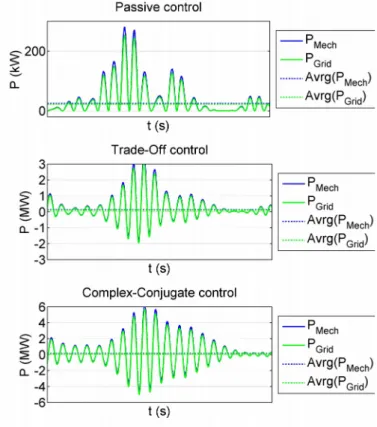
Fig. 11. Example of power time series for a given random draws for the excitation force phases. The graphs compare the three control strategies: Complex-Conjugate (C-C) (ccontrol = 0), Passive (P) (ccontrol → 1) and

Trade-Off (T-O) (ccontrol= closs = 0.1). The loss coefficient is closs = 0.10,

the sea-state is Tp = 9.5 s and Hs = 2.5 m. The constraint for stability is

weak (see (56) and (57)). Note that the scale for the power in the three case are not the same.

Production maximization is not the ultimate goal of these control strategies. Given the over-sizing required to achieve the production maximization, the solution with maximum grid power is not optimal for per-kWh cost. A complete study of the cost of both the generator and its converter is needed in order to draw a conclusion on the best control strategy.

We can reasonably suppose that the peak and root mean square value of the force are correlated with the linear generator cost. Fig. 12 (b) therefore depicts the two following ratios for comparing these various solutions:

rf rms= fPTO rms Pgrid and rf peak= f PTO peak Pgrid (61)

We can also reasonably suppose that the peak and root mean square value of the mechanical power are correlated with the converter cost. Fig. 12 (c) then represents the two following ratios for comparing these various solutions:

rP rms= Pmech rms Pgrid and rP peak= Pmech peak Pgrid (62)

V. CONCLUSIONAND OUTLOOK

This paper has focused on the potential resource for a Direct Wave Energy Converter, in a global context of kWh cost minimization. Electrical chain losses and force or power amplitude constraints play an important role in designing the electric chain, and hence in its cost. Moreover, they play a key role in the conversion mechanism. For this reason, the control strategy and the electric chain design are highly correlated.

This paper has proven that taking account of electrical losses in the design of a control strategy improves global efficiency of the conversion chain compared to classical solutions, i.e.: a passive strategy or complex conjugate strategy. Power and force leveling must be tested with this strategy in order to minimize the chain size introduced to achieve a given production.

Converted energy maximization may help to minimize the per-kWh cost; however recovery optimization is not an end in itself. The final system, including the electric chain and control strategy, must minimize the per-kWh cost. In the case presented here, the continuous variation of a control parameter offers multiple possibilities. Economic considerations must be taken into account when approximating the per-kWh cost optimization.

ACKNOWLEDGMENT

This work has been financed by the French National Research Agency (ANR) within the project “QUALIPHE” (power quality and grid integration of direct wave energy converters), which is part of the "PROGELEC" program.

REFERENCES

[1] World Energy Council, “Survey of Energy Resources,”

2010 Survey of Energy Resources, vol. 2010 Surve. pp.

543–602, 2010.

[2] N. J. Baker and M. A. Mueller, “Direct drive wave energy converters,” Revue des Energies Renouvelables, pp. 1–7, 2001.

[3] J. Aubry, H. Ben Ahmed, B. Multon, A. Clément, and A. Babarit, “Classification of wave energy converters,” in

Marine Renewable Energy Handbook, John Wiley., B.

MULTON, Ed. 2011, pp. 324–363.

[4] J. K. H. Shek, D. Macpherson, M. A. Mueller, and J. Xiang, “Reaction force control of a linear electrical generator for direct drive wave energy conversion,”

Renewable Power Generation, IET, vol. 1, no. 1, pp. 17–

24, 2007.

(a)

(b)

(c)

Fig. 12. (a) Average losses vs. average production; (b) Ratio between peak and root mean square values for the Power Take-Off force and average production power vs. average production power; (c) Ratio between peak and root mean square values for the Power Take-Off force and average production power vs. average production power. All the three graphs are subject to the same conditions: the loss coefficient is closs = 0.10, the

sea-state is Tp = 9,5 s and Hs = 2,5 m. The control coefficient ccontrol varies

from 0.1 to 1.0. Blue lines correspond to the solutions without stability constraints (w/o c.), green lines with weak stability constraints (wc) and red line with strong stability constraints (sc).

[5] G. Li, G. Weiss, M. Mueller, S. Townley, and M. R. Belmont, “Wave energy converter control by wave prediction and dynamic programming,” Renewable

Energy, vol. 48, pp. 392–403, Dec. 2012.

[6] E. Tedeschi and M. Molinas, “Tunable Control Strategy for Wave Energy Converters With Limited Power Takeoff Rating,” IEEE Transactions on Industrial Electronics, vol. 59, no. 10, pp. 3838–3846, Oct. 2012.

[7] E. Tedeschi, M. Carraro, M. Molinas, and P. Mattavelli, “Effect of Control Strategies and Power Take-Off Efficiency on the Power Capture From Sea Waves,” IEEE

Transactions on Energy Conversion, vol. 26, no. 4, pp.

1088–1098, Dec. 2011.

[8] J. Aubry, M. Ruellan, H. Ben Ahmed, and B. Multon, “Minimization of the kWh cost by optimization of an all-electric chain for the SEAREV Wave Energy Converter.,” in 2nd International Conference on Ocean Energy, 2008. [9] J. Falnes, Ocean Waves and Oscillating Systems: Linear

Interactions Including Wave-Energy Extraction.

Cambridge University Press, 2012.

[10] W. E. Cummins, “The Impulse Response Function and Ship Motions,” in Symposium on Ship Theory, 1962. [11] G. Delhommeau, “Seakeeping codes aquadyn and

aquaplus,” Proc. of the 19th WEGEMT school, numerical

simulation of hydrodynamics: ships and offshore structures, 1993.

[12] A. H. Clément and A. Babarit, “Discrete control of

resonant wave energy devices.,” Philosophical

transactions. Series A, Mathematical, physical, and engineering sciences, vol. 370, no. 1959, pp. 288–314,

Jan. 2012.

[13] P. Nebel, “Maximizing the efficiency of wave-energy plant using complex-conjugate control,” Engineers, Part

I: Journal of Systems and Control, vol. 206, 1992.

[14] M. Ruellan, H. Ben Ahmed, B. Multon, C. Josset, A. Babarit, and A. H. Clément, “Design Methodology for a SEAREV Wave Energy Converter,” IEEE Transactions

on Energy Conversion, vol. 25, no. 3, pp. 760–767, Sep.

2010.

[15] H. S. Lee and S. D. Kim, “A comparison of several wave spectra for the random wave diffraction by a semi-infinite breakwater,” Ocean Engineering, vol. 33, no. 14–15, pp. 1954–1971, Oct. 2006.

[16] A. Babarit, J. Hals, M. J. Muliawan, a. Kurniawan, T. Moan, and J. Krokstad, “Numerical benchmarking study of a selection of wave energy converters,” Renewable