Études de l’effet tunnel des spins quantiques macroscopiques
par
Solomon Akaraka Owerre
Département de physique Faculté des arts et des sciences
Thèse présentée à la Faculté des études supérieures en vue de l’obtention du grade de Philosophiæ Doctor (Ph.D.)
en Faculté des arts et des sciences
October, 2014
c
Université de Montréal Faculté des études supérieures
Cette thèse intitulée:
Études de l’effet tunnel des spins quantiques macroscopiques
présentée par: Solomon Akaraka Owerre
a été évaluée par un jury composé des personnes suivantes: Andrea Bianchi, président-rapporteur
Manu Paranjape, directeur de recherche
Luc Vinet, membre du jury
André-Marie Tremblay, examinateur externe
Véronique Hussin, représentant du doyen de la FES
This thesis presents recent theoretical analyses together with experimental observa-tions on macroscopic quantum tunneling and quantum-classical phase transiobserva-tions of the escape rate in large spin systems. We consider biaxial ferromagnetic spin systems. Using the coordinate dependent spin coherent state path integral, we obtain the quantum phase interference and the energy splitting of these systems. We also present a lucid exposition of tunneling in antiferromagnetic exchange-coupled dimer, with easy-axis anisotropy. Indeed, we obtain the ground state, the first excited state, and the energy splitting, for both integer and half-odd integer spins. These results are then corroborated using per-turbation theory and the coordinate independent spin coherent state path integral. We further present a lucid explication of the effective potential method, which enables one to map a spin Hamiltonian onto a particle Hamiltonian; we employ this method to our models, however, in the presence of an applied magnetic field. This method enables us to investigate quantum-classical phase transitions of the escape rate of these systems. We obtain the phase boundaries, as well as the crossover temperatures of these phase transi-tions. Furthermore, we extend our analysis to one-dimensional anisotropic Heisenberg antiferromagnet, with N periodic sites. For even N, we show that the ground state is non-degenerate and given by the coherent superposition of the two Neél states. For odd
N, however, the Neél state contains a soliton; as the soliton can be placed anywhere
along the ring, the ground state is, indeed, N-fold degenerate. In the perturbative limit (weak exchange interaction), quantum fluctuation stemming from the interaction term lifts this degeneracy and reorganizes the states into a band. We show that this occurs at order 2s in (degenerate) perturbation theory. The ground state is non-degenerate for inte-ger spin, but degenerate for half-odd inteinte-ger spin, in accordance with Kramers’ theorem [72].
Keywords: Perturbation theory, effective potential, antiferromagnet, single molecule magnets, instanton, soliton, energy splitting, phase transition, path integral.
RÉSUMÉ
Dans cette thèse, nous présentons quelques analyses théoriques récentes ainsi que des observations expérimentales de l’effet tunnel quantique macroscopique et des tran-sitions de phase classique-quantique dans le taux d’échappement des systèmes de spins élevés. Nous considérons les systèmes de spin biaxial et ferromagnétiques. Grâce à l’approche de l’intégral de chemin utilisant les états cohérents de spin exprimés dans le système de coordonnées, nous calculons l’interférence des phases quantiques et leur distribution énergétique. Nous présentons une exposition claire de l’effet tunnel dans les systèmes antiferromagnétiques en présence d’un couplage d’échange dimère et d’une anisotropie le long de l’axe de magnétisation aisé. Nous obtenons l’énergie et la fonc-tion d’onde de l’état fondamentale ainsi que le premier état excité pour les systèmes de spins entiers et demi-entiers impairs. Nos résultats sont confirmés par un calcul utilisant la théorie des perturbations à grand ordre et avec la méthode de l’intégral de chemin qui est indépendant du système de coordonnées. Nous présentons aussi une explica-tion claire de la méthode du potentiel effectif, qui nous laisse faire une applicaexplica-tion d’un système de spin quantique vers un problème de mécanique quantique d’une particule. Nous utilisons cette méthode pour analyser nos modèles, mais avec la contrainte d’un champ magnétique externe ajouté. La méthode nous permet de considérer les transitions classiques-quantique dans le taux d’échappement dans ces systèmes. Nous obtenons le diagramme de phases ainsi que les températures critiques du passage entre les deux régimes. Nous étendons notre analyse à une chaine de spins d’Heisenberg antiferro-magnétique avec une anisotropie le long d’un axe pour N sites, prenant des conditions frontière périodiques. Pour N paire, nous montrons que l’état fondamental est non-dégénéré et donné par la superposition des deux états de Néel. Pour N impair, l’état de Néel contient un soliton, et, car la position du soliton est indéterminée, l’état fondamen-tal est N fois dégénéré. Dans la limite perturbative pour l’interaction d’Heisenberg, les fluctuations quantiques lèvent la dégénérescence et les N états se réorganisent dans une
bande. Nous montrons qu’à l’ordre 2s, où s est la valeur de chaque spin dans la théorie des perturbations dégénérées, la bande est formée. L’état fondamental est dégénéré pour s entier, mais deux fois dégénéré pour s un demi-entier impair, comme prévu par le théorème de Kramer[72].
Mots clés: théorie des perturbations, potentiel effectif, antiferromagnétique, instanton, soliton, de l’enchevêtrement, transition de phase, intégrale de chemin.
CURRICULUM VITÆ
Education
2014 Ph.D., in Physics; Université de Montréal
2011 M.Sc., in Physics; Perimeter Institute for Theoretical Physics (University of Waterloo)
2010 M.Sc., in Mathematical Sciences; African Institute for Mathematical Sciences (University of Cape Town)
2008 B.Sc., in Physics; Michael Okpara University of Agriculture Publications
I) S. A. Owerre and M. B. Paranjape: “Haldane-like antiferromagnetic spin chain in
the large anisotropy limit". Phys. Lett. A,378, 3066 (2014)
II) S. A. Owerre and M. B. Paranjape: “Phase transition between quantum and
clas-sical regimes for the escape rate of dimeric molecular nanomagnets in a staggered magnetic field". Phys. Lett. A,378, 1407 (2014)
III) S. A. Owerre and M. B. Paranjape: “Macroscopic quantum tunneling and phase
transition of the escape rate in spin systems". To be published in Physics Reports.
ArXiv:1403.4208 (2014)
IV) S. A. Owerre: “Rotating Entangled States of an Exchange-Coupled Dimer of
Single-Molecule Magnets". J. Appl. Phys.115 , 153901 (2014)
V) S. A. Owerre and M. B. Paranjape: “Quantum-classical transition of the escape
rate of a biaxial ferromagnetic spin". J. Magn. Magn. Mater.93, 358, (2014) VI) S. A. Owerre and M. B. Paranjape: “Coordinate (in)dependence and quantum
in-teference in quantum spin tunnelling". Submitted to Physica B. ArXiv:1309.6615
VII) S. A. Owerre and M. B. Paranjape: “Macroscopic Quantum Tunnelling of Two
Interacting Spins". Phys. Rev. B,88, 220403(R) (2013)
VIII) S. A. Owerre: “Spin Wave Theory of XY Model with Ring Exchange Interaction on
a Triangular Lattice". Can. J. Phys.91, 542 (2013)
IX) S. A. Owerre: “Effects of Magnetic field on Macroscopic Quantum Tunnelling". Can. J. Phys.91, 722, 2013
CONTENTS
ABSTRACT . . . . iii
RÉSUMÉ . . . . iv
CURRICULUM VITÆ . . . . vi
CONTENTS . . . viii
LIST OF FIGURES . . . xii
LIST OF APPENDICES . . . xviii
LIST OF ABBREVIATIONS . . . xix
NOTATION . . . xx
DEDICATION . . . xxi
ACKNOWLEDGMENTS . . . xxii
CHAPTER 1: INTRODUCTION . . . . 1
1.1 The concept of quantum tunneling . . . 1
1.2 Quantum tunneling in single molecule magnets . . . 2
1.3 Quantum-classical phase transitions of the escape rate . . . 4
1.4 Quantum tunneling in one-dimensional antiferromagnetic molecular mag-nets . . . 7
CHAPTER 2: PATH INTEGRAL . . . . 9
2.1 Introduction . . . 9
2.2.1 Imaginary time path integral formalism . . . 14
2.2.2 Instantons in the double well potential . . . 15
2.3 Spin coherent state path integral . . . 20
2.3.1 Coordinate independent form . . . 20
2.3.2 Coordinate dependent form . . . 25
2.4 Conclusion and Discussion . . . 28
CHAPTER 3: QUANTUM TUNNELING OF LARGE SPIN SYSTEMS . 29 3.1 Introduction . . . 29
3.2 Quantum tunneling in biaxial ferromagnetic spin models . . . 30
3.2.1 Biaxial ferromagnetic spin model with y-easy axis . . . . 30
3.2.2 Biaxial spin model with an external magnetic field . . . 33
3.2.3 Experimental observations . . . 37
3.2.4 Biaxial ferromagnetic spin model with z-easy axis . . . . 39
3.3 Macroscopic quantum tunneling in antiferromagnetic dimer model . . . 43
3.3.1 Model Hamiltonian . . . 43
3.3.2 Spin coherent state path integral analysis . . . 44
3.4 Coordinate independent formalism . . . 49
3.4.1 Classical equations of motion in coordinate independent form . 50 3.4.2 Wess Zumino term in coordinate independent form . . . 51
3.4.3 Coordinate independent biaxial spin system . . . 53
3.5 Conclusion and Discussion . . . 55
3.6 Article for coordinate independent analysis . . . 57
3.7 Article for the two interacting dimer model . . . 63
CHAPTER 4: ROTATING ENTANGLED STATES OF AN EXCHANGE-COUPLED DIMER . . . 69
4.1 Introduction . . . 69
x
4.3 Effects of a staggered magnetic field . . . 72
4.4 The effects of an environmental coupling . . . 74
4.5 Rotation, Interaction and Environment . . . 77
4.6 Conclusion and Discussion . . . 82
4.7 Article for rotating entangled states of an antiferromagnetic dimer model. 84 CHAPTER 5: EFFECTIVE POTENTIAL METHOD AND ESCAPE RATE 91 5.1 Introduction . . . 91
5.2 From spin Hamiltonian to particle Hamiltonian . . . 92
5.2.1 Effective potential method for a uniaxial spin model . . . 92
5.2.2 Effective potential method for the XOY -easy-plane model . . . 97
5.3 Methods for studying quantum-classical phase transitions of the escape rate . . . 100
5.3.1 Phase transition with thermon action . . . 101
5.3.2 Phase transition with thermon period of oscillation . . . 103
5.3.3 Phase transition with free energy . . . 104
5.3.4 Phase transition with criterion formula . . . 104
5.4 Conclusion and Discussion . . . 106
CHAPTER 6: QUANTUM-CLASSICAL PHASE TRANSITIONS OF THE ESCAPE RATE IN LARGE SPIN SYSTEMS . . . 107
6.1 Introduction . . . 107
6.2 Phase transition in a biaxial model with a medium axis magnetic field . 109 6.2.1 Model Hamiltonian . . . 109
6.2.2 Particle mapping . . . 110
6.2.3 Vacuum instanton trajectory . . . 112
6.2.4 Phase boundary and crossover temperatures . . . 113
6.2.5 Free energy with a magnetic field . . . 117
6.3.1 Model Hamiltonian . . . 119
6.3.2 Effective potential of the model Hamiltonian . . . 122
6.3.3 Analysis with zero staggered magnetic field . . . 127
6.3.4 Analysis with a staggered magnetic field . . . 142
6.4 Conclusion and Discussion . . . 151
6.5 Article for quantum-classical phase transition in ferromagnetic spin sys-tems . . . 152
6.6 Article for quantum-classical phase transition in anti-ferromagnetic dimer model . . . 159
6.7 Review article to appear in Physics Reports . . . 169
CHAPTER 7: ONE-DIMENSIONAL QUANTUM LARGE SPIN CHAIN 234 7.1 Introduction . . . 234
7.2 Spin wave theory . . . 236
7.3 Even number of sites . . . 237
7.3.1 Classical trajectory for even number of sites . . . 238
7.3.2 Energy splitting and low-lying eigenstates . . . 240
7.4 Odd number of sites . . . 242
7.4.1 Soliton in odd spin chain . . . 242
7.4.2 Perturbation theory for odd spin chain . . . 243
7.4.3 Energy band . . . 245
7.4.4 Effect of a transverse magnetic field . . . 250
7.5 Conclusion and Discussion . . . 252
7.6 Article for one-dimensional quantum large spin chain . . . 254
CONCLUSION . . . 260
LIST OF FIGURES
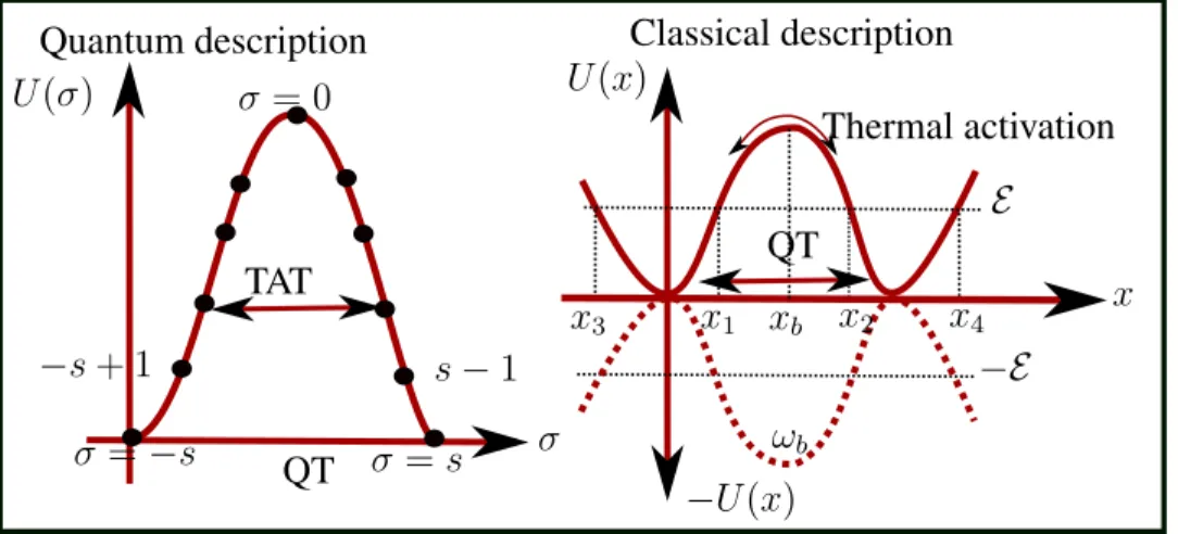
1.1 Left: Quantum description of a single spin Hamiltonian of the form ˆH = −D ˆS2
z + ˆH?, where D > 0 and ˆH?is quadratic in ˆS. The free term gives a potential of U(σ) = −Dσ2 using the state |σi. The presence of the perturbative term ˆH?splits the two
low-est degenerate ground states σ = ±s via quantum tunneling (QT). Transitions between existed states occur via thermal assisted quan-tum tunneling (TAT). Right: The description of the same Hamil-tonian using instanton technique via semiclassical methods (spin coherent state path integral or the effective potential method). . . 4 2.1 A sketch of an inverted double well potential with two minima at
±a. There are two trivial solutions corresponding to a fixed motion
of the particle at the top of the left or right hill of the potential. Tunneling is achieved by a nontrivial solution in which the particle starts at the top of the left hill at ⌧ ! −1 and roll through the dashed line and emerges at the top of the right hill at ⌧ ! +1. Such a solution is called an instanton. . . 16 2.2 The directions of the unit vectors ˆz and ˆn on a two-sphere . . . 21 2.3 The directions of the unit vectors ˆn1, ˆn2, ˆn3 forming the area of a
spherical triangle. . . 22 3.1 The description of a classical spin (thick arrows) on a two-sphere
with two classical ground states. For hz = 0, ✓ = ±⇡/2, the two classical ground states lie in the ±y directions which are joined by two tunneling paths in the equator. For hz > 0, ✓ = ± arccos ↵,
3.2 Oscillation of the tunneling splitting as a function of the magnetic field parameter ↵, with λ = 0.03. Reproduced from [1] . . . . 36 3.3 Measured tunnel splittings obtained by the Landau-Zener method
as a function of transverse field for all three SMMs. The tunnel splitting increases gradually for an integer spin, whereas it in-creases rapidly for a half-integer spin. Adapted with permission from Wernsdorfer et. al[143]. . . . 37 3.4 Measured tunneling splitting as a function of the applied field for
the Hamiltonian ˆH =−AS2
z+ B(Sx2− Sy2)− gµBH?(Sxcos ' +
Sysin '). Top figure (A) is the quantum transition between m =
±10 and several values of the azimuth angles '. Bottom figure
(B) is for ' ⇡ 0◦ and quantum transition between m = −10 and m = 10 − n, where n = 0, 1, 2, · · · , m = −s, · · · , s, and
s = 10. A = 0.275K, B = 0.046K for Fe8 molecular cluster.
This Hamiltonian is related to that of Eqn.(3.11) by D = A + B and E = A − B. Adapted with permission from Wernsdorfer and Sessoli [140]. . . 38 3.5 The description of a classical spin (thick arrows) on a two-sphere
S2 with two classical ground states pointing along the ±ˆz
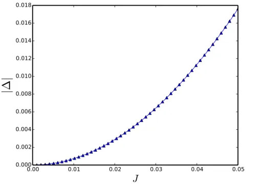
direc-tions. Tunneling corresponds to the rotation of the spins in the reverse direction. . . 41 3.6 The plot of the ground state energy splitting against J obtained
from exact diagonalization for D = 1 and s1 = s2 = s = 13/2. . . 48
4.1 The plot of |C(t)| against time for ohmic d = 1 and super-Ohmic
d = 2, 3 dissipations. The function reaches a maximum of one
and decays to zero at long times for the ohmic dissipation but it is never decays to zero for the super-ohmic dissipation. . . 76
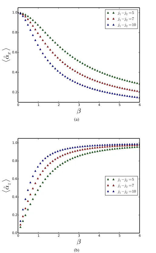
xiv 4.2 The expectation values of hˆ↵xi and hˆ↵zi plotted against the
param-eter β with s = 9/2. . . . 80 4.3 The plot of staggered magnetic moment against β with s = 9/2. . 81 5.1 The tridiagonal sparse matrix representation of 21 ⇥ 21 matrix for
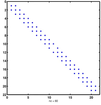
s = 10, with 60 nonzero values. . . 93
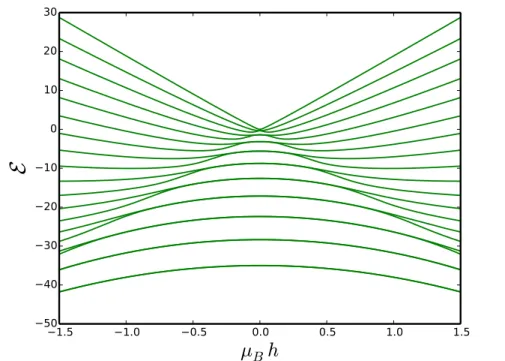
5.2 The exact diagonalization of Eqn.(5.6) for s = 10 and D = 0.35. At h = 0, the states are labeled by σ = ±10, ±9, · · · , 0. There are 21energy level which are split by the magnetic field. The splitting in the perturbative limit h ⌧ D is ⇠ (h/D)2s, which evidently is
very small to be observed in the diagram. . . 94 6.1 The plot of the effective potential, Eqn.(6.9) for ↵x = 0.1, λ = 0.2.
For this potential xsb = 0and xlb = 2K(0.2). . . 111
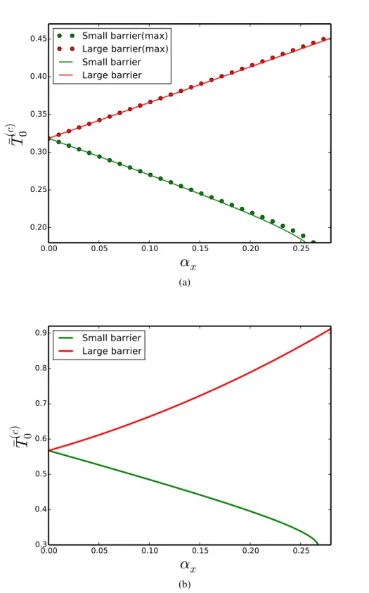
6.2 The phase diagram − vs ↵x at the phase boundary (a): Small barrier. (b): Large barrier. . . 115 6.3 Colour online: Dependence of the crossover temperatures on the
magnetic field at the phase boundary: (a) Second-order and its maximum for the small and large barrier, (b) First-order for the small and the large barrier. These graphs are plotted with T(c)
0 =
T0(c)/D2˜s. . . 116
6.4 The numerical plot of the free energy for = 0.8 and ↵ = 0.05. . 118 6.5 Hysteresis loops for the [Mn4]2 dimer at several field sweep rates
and 40 mK. The tunnel transitions are labeled from 1 to 5 corre-sponding to the plateaus. Adapted with permission from Tiron et.
al [134] . . . 121
6.6 Plot of energy vs. staggered magnetic field of Eqn.(6.44) for sA=
sB = 9/2, J = 0.95, and D = 0.01. . . 123 6.7 The plot of the potential for several values of with D = 1. . . . 128
6.8 The periodic instanton trajectory with λ = 0.2. . . 131 6.9 Dependence of the actions on temperature. The top figure is for
first-order phase transition with the experimental parameters[121, 134]: s = 9/2; D = 0.75; = 0.16. The bottom figure is for second- order phase transition with; s = 9/2; D = 0.75; = 1.12. 135 6.10 The plot of the position dependent mass in Eqn.(6.60) for several
values of with D = 1. . . 136 6.11 The effective free energy of the escape rate vs. Q for = 0.4 and
several values of ✓ = T/T(2)
0 , first-order transition. . . 138
6.12 The period of oscillation vs. Q, using the experimental parameters in [121, 134]: s = 9/2; D = 0.75K; J = 0.12K ) = 0.16 (first-order transition). Inset = 1.16 (second-order transition).
β0(1) and β0(2) are the actual crossover temperatures for first- and
second-order phase transitions respectively. . . 140 6.13 Zero magnetic field crossover temperatures plotted against . The
functions increase rapidly as varies between 0 and 1. ¯T0 = ⇡T0(1,2)/Ds . . . 141
6.14 The plot of the effective potential and its inverse as a function of r for = 0.6 and ↵ = 0.15. . . 143 6.15 Colour online: The phase diagram of ↵c vs. c. In the regime
of first-order phase transition, I < 0; in the regime of second-order transition, I > 0; of course, I = 0 at the phase boundary, indicated by the green line. . . 144 6.16 Colour online: The numerical plot of the free energy with = 0.4
and ↵ = 0.15. The phase transition from thermal to quantum regimes occurs at ✓ = 1.044, which is smaller than that of zero magnetic field, ✓ = 1.054. . . 146
xvi 6.17 Colour online: The period of oscillation vs. Q with; s = 9/2;
D = 0.75; = 0.16 (first-order transition) and different values of ↵.147
6.18 Dependence of the thermon and thermodynanmic actions on tem-perature, with the experimental paramters[121, 134]: s = 9/2;
D = 0.75; = 0.16; ↵ = 0.2 (first-order transition). . . 148
6.19 Three dimensional plot of the Landau coefficient b. Region of first-order phase transition b < 0. Second-first-order transition b > 0. The phase boundary b = 0 is placed on the bottom plane for proper view of the top plane. . . 149 6.20 The crossover temperatures at the phase boundary between
first-and second-order transitions plotted against ↵c, where ¯T0(c) = T0(c)/D˜s.
. . . 150 7.1 A sketch of the classical anisotropy energy, with two degenerate
minima. The two degenerate Néel states are localized in each min-imum. Due to tunneling between them, they recognize into sym-metric and antisymsym-metric coherent superpositions separated by an energy splitting. In the thermodynamic limit, the splitting vanishes and the two Néel states become the degenerate ground states. . . . 241 7.2 The first Brillouin zone of the one-soliton energy band. Due to
hopping of the soliton, the lattice spacing has increased by 2a. Thus, the first Brillouin zone is halved with boundaries q = ±⇡
2a,
7.3 Color online: The plot of the one-soliton energy band in the first reduced Brillouin zone. The bandwidth is 4|CJ|. For half-odd integer spins, the ground state is doubly degenerate (black spots), with "0 = −2|CJ|; these states can be regarded as the Kramers’ doublets [72]. While for integer spins, the ground state (black spot) is non-degenerate, with "0 =−2|CJ|. . . 249
LIST OF APPENDICES
SMMs Single molecule magnets
SQUID Superconducting quantum interference devices RHS Right hand side
EP Effective potential WZ Wess Zumino
Re The real part of a complex function WKB Wentzel–Kramers–Brillouin
NOTATION
sn(x, λ), cn(x, λ), dn(x, λ) Jacobi elliptic functions
µm, µB, and µ Magnetic moment, Bohr magneton and reduced mass respectively !p, !b, and !0 Periodic instanton, sphaleron and vacuum instanton frequencies
T , T , and T Time-ordered operator, temperature, and kinetic energy respectively SE, Sp and B Euclidean, periodic instanton and vacuum instanton actions respectively
K(λ) and F (', λ) Complete and incomplete elliptic integrals of the first kind
⇧(γ2; λ) Complete elliptic integral of the third kind
λand ↵ Dimensionless anisotropy and magnetic field parameters LE and L Euclidean and Minkowski Lagrangian respectively
PE and P Euclidean and Minkowski propagators respectively
δ(p− p0) Dirac delta function
S2 2-sphere H Hilbert space
⌧ Euclidean or imaginary time
β Inverse temperature (period of oscillation) E Energy of a particle U Potential energy ˆ x Position operator ˆ p Momentum operator ˆ H Hamiltonian operator ⌘ Frictional constant Z Set of integers
ACKNOWLEDGMENTS
First and foremost, I would like to thank God for His unprecedented grace and prov-idence. His infinite mercies have been indispensable during my studies. The success of completing my Ph.D. degree program is not a personal achievement, rather it is a col-lective one. It will be an unforgivable act not to appreciate the people that contributed immensely to this successful journey.
This journey started back in 2010 at the African Institute for Mathematical Sciences (AIMS), Cape Town, South Africa, where I met my supervisor Prof. Manu Paranjape, when he gave his specialized course on instantons and tunneling. At this time it never came to my mind that I would be his Ph.D. student. Fortunately, I met him again at Perimeter Institute for theoretical Physics (PI), where he is a member. When I finished my masters at PI in 2011, he offered me a Ph.D. position in his group at the Université de Montréal. It was indeed a great change of scenery, and a reminiscent of his approach of teaching at AIMS, which I have invariably admired. He has a great decency and good sense of humour; he cares about his students’ welfare; he pays attention to their complaints and he gives good advice like a father. I am grateful for working with him as a student and I greatly appreciate all his kindness towards me.
It goes without saying that the prestigious AIMS paved the way for this international collaboration. I would like to appreciate the support of Prof. Neil Turok during my stay at PI. Of course, it goes without saying that I benefited from the financial support of Natural Sciences and Engineering Research Council of Canada (NSERC), through my supervisor’s grant, for the whole period of my studies, and from the Faculté des études supérieures et postdoctorales (FESP) and the department of physics. In the course of my Ph.D., I got some publications with my supervisor; I would like to appreciate the inputs of Prof. Sung-Sik Lee, Prof. Ian Affleck, and Prof. Richard Mackenzie, whom my supervisor conversed with, concerning my research and publications.
program. I appreciate useful discussions with Joachim Nsofini, in many areas of physical activities. He has been a very good friend since our stay at PI. I would like to appreciate a lovely lady, Kesha Fatmata Senessie, who has supported me since the beginning of my program. I would also like to thank my office mates, Gendron Marsolais Marie-Lou and Saoussen Mbarek, for their immense contribution to my student life.
Last but not least, I greatly appreciate all the support and the parental care from my family. I’m grateful for the support of my mother, Charity Owerre; my late father, Mark Chinyere Owerre; my aunt and her husband, Mr Chikezie and Dr. Mrs. Nkem Ogbonna; all my siblings, whom I cannot list their names without exceptions. Needless to say, you played a decisive role in my academic pursuit. You really inspired me. You motivated me. You continued to pray for me. I love you all and I pray that God will continue to enrich us with His divine blessing.
CHAPTER 1
INTRODUCTION
Anyone who is not shocked by the quantum theory has not understood it.
Niels Bohr
1.1 The concept of quantum tunneling
Quantum tunneling, being one of the most remarkable manifestations of quantum mechanics, is a ubiquitous phenomenon in physics. It involves the presence of a po-tential barrier, that is the region where the popo-tential energy is greater than the energy of the particle. Classically, tunneling of a particle through this barrier is prohibited, as it requires the particle to have a negative kinetic energy. However, quantum mechani-cally, one finds a nonzero probability for finding the particle in the classically forbidden region. Thus, a quantum particle can tunnel through the barrier. The fundamental con-cept of this phenomenon is based on two formalisms: path integral formalism (instanton techniques) [33, 34, 39, 40, 61, 62, 64, 78, 116, 117] and Wentzel-Kramers-Brillouin (WKB) formalism [76] . In one-dimensional systems, the tunneling amplitude (whose modulus squared gives the probability) is usually computed by these two fundamental formalisms. For particle in a double well potential with two degenerate minima, the ba-sic understanding is that in the absence of tunneling, the clasba-sical ground states of the system, which correspond to the minima of the potential, remain degenerate. Tunneling between these minima lifts the degeneracy; the true ground state and the first excited state become the symmetric and the antisymmetric linear superposition of the classical ground states respectively, with an energy splitting between them[34, 76]. In general, the two minima of the potential are not degenerate; the state with lower energy is the
true vacuum, while the state with higher energy is the false vacuum. The false vacuum is rendered unstable due to quantum tunneling; thus, the interesting object to compute is the decay rate of the false vacuum[32, 33]. Such a scenario plays a vital role in cosmol-ogy, especially in the theory of early universe and inflation. Besides, in some quantum systems, tunneling does not involve the splitting of the classical ground states or the decay of the false vacuum, but rather a dynamic oscillation of the (phase) difference between two macroscopic order parameters [35], which are separated by a thin normal layer, through tunneling of the macroscopic effective excitations, such as Cooper pairs as in Josephson effect[38, 65].
1.2 Quantum tunneling in single molecule magnets
In the last few decades, the phenomenon of macroscopic quantum tunneling has been extended to other branches of physics. Quantum tunneling of spins has been predicted in molecular magnets, such as MnAc12, Mn12, and Fe8[24, 87, 136, 140, 145]. These
sin-gle molecule magnets (SMMs) are composed of several molecular magnetic ions, whose spins are coupled by intermolecular interactions, giving rise to an effective single giant spin, which can tunnel through its magnetic anisotropy barrier; hence the name “macro-scopic quantum spin tunneling1". The study of macroscopic quantum tunneling in these
systems stems from the work of Hemmen and Süt˝o [136]. They studied the tunneling in a uniaxial ferromagnetic spin model with an applied magnetic field, using the WKB method. Enz and Schilling [87] considered a biaxial ferromagnetic spin model with a magnetic field via the instanton technique. Subsequently, Chudnovsky and Gunther [24] studied many ferromagnetic spin systems comprehensively, by solving the instanton tra-jectory of the Landau Lifshitz equation. These studies were based upon a semiclassical description, that is by representing the spin operator as a unit vector parameterized by
1In most literatures, macroscopic quantum tunneling refers to tunneling in a bias (metastable) potential, while macroscopic quantum coherence refers to tunneling in a potential with degenerate minima [81]. In this thesis we will use the former to refer to both systems.
3 spherical coordinates.
In this description, the spin is considered as a particle on a two-dimensional sphere
S2, however, in the presence of a topological term, called the Berry’s phase term or
Wess-Zumino action [12, 146, 147], which effectively corresponds to the magnetic field of a magnetic monopole at the centre of the two-sphere. Based on this semi-classical description, it was predicted serendipitously, that for integer spins tunneling is allowed, while for half-odd integer spin tunneling is completely suppressed at zero (external) magnetic field [56, 86]. The vanishing of tunneling for half-odd integer spins is under-stood as a consequence of destructive interference between tunneling paths, which is directly related to Kramers’ degeneracy[72, 95], due to the time reversal invariance of the Hamiltonian. In the presence of a magnetic field applied along the spin hard axis, Garg [1] showed that the tunneling splitting does not vanish for half-odd integer spins, rather it oscillates with the field, only vanishes at a certain critical value of the field. In this case, suppression of tunneling is not related to Kramers’ degeneracy due to the pres-ence of a magnetic field. These serendipitous theoretical predictions were subsequently observed experimentally in Fe8 molecular cluster [125, 140, 142]. As the semiclassical
approach is valid for large spin systems, an exact mapping of spin systems onto a particle problem was considered by Scharf et al [123] and Zaslavskii [148, 150]. They studied the exact mapping of a spin Hamiltonian onto a particle Hamiltonian, which has a mass and a potential field (Schrödinger equation). This method is called the “effective poten-tial method”. It gives the possibility of investigating spin tunneling akin to tunneling in one-dimensional double well potential. Recently, the problem of a rotating molecular magnet has attracted considerable attention. A theoretical study of this problem has been investigated for ferromagnets [29, 67], and for antiferromagnets [102].
1.3 Quantum-classical phase transitions of the escape rate
The possibility of quantum tunneling requires a very low temperature, T ! 0. This leads to a temperature independent transition amplitude, governed by Γ = Ae−B, where
B is the instanton action and A is a pre-factor. At high temperature, quantum tunneling
becomes inconsequential; then the particle has the possibility of crossing over the barrier, a process called classical thermal activation, which dates back to the work of Kramers [73], for the diffusion of a particle over the barrier. A review on this subject for both particles and spin systems can be found in many literatures[31, 109, 127]. The transition amplitude for a classical thermal activation is governed by the Van’t Hoff-Arrhenius Law [109], Γ = Be−β U, where ∆U is the height of the potential barrier, β is the inverse temperature, and B is a pre-factor.
QT !b E −E x4 x3 x1 xb x2 U (x) −U(x) Thermal activation σ =−s s− 1 −s + 1 σ = 0 TAT
Quantum description Classical description
σ = s
x
σ U (σ)
QT
Figure 1.1: Left: Quantum description of a single spin Hamiltonian of the form ˆH = −D ˆS2
z + ˆH?, where D > 0 and ˆH?is quadratic in ˆS. The free term gives a potential of
U (σ) = −Dσ2 using the state |σi. The presence of the perturbative term ˆH
? splits the two lowest degenerate ground states σ = ±s via quantum tunneling (QT). Transitions between existed states occur via thermal assisted quantum tunneling (TAT). Right: The description of the same Hamiltonian using instanton technique via semiclassical methods (spin coherent state path integral or the effective potential method).
The basic understanding of quantum-classical phase transitions of the escape rate is as follows: for a particle in a metastable cubic potential or double well quartic parabolic
5 potential, denoted by U(x), with no environmental influence (dissipation), transition at finite temperature is dominated by thermon (periodic) instanton trajectory2, whose action
is denoted by Sp(E) [20], where E is the energy of the particle in the inverted potential
−U(x). The escape rate is defined by taking the Boltzmann average over tunneling
probabilities at finite energy, weighed by the exponential of Sp(E) [6]. At the bottom of the barrier we have Sp(E) ! S(Umin), where S(Umin)is the action at the bottom of the
barrier, while at the top of the barrier, Sp(E) ! S0 = β∆U, which is the action of a
constant trajectory at the top of the barrier. Now, if we compare the plot of the thermon action Sp, and that of the thermodynamic action S0, against temperature[20], the “critical
temperature Tc" at the intersection defines the crossover or phase transition temperature from thermal regime to quantum regime.3 If this intersection is sharp, Tc can be thought of as a first-order “phase transition" (crossover) temperature, from classical (thermal) to quantum regimes. At Tc ⌘ T(1)
0 , there is a discontinuity in the first-derivative of the
action Sp[50]. The approximate form of this crossover temperature can be estimated by equating the quantum action S(Umin), at the bottom of the barrier, and that of the
classical action at the top of the barrier S0, [127]:4
T0(1) = 1 β0(1) = ∆U S(Umin) = ∆U 2B . (1.1)
For a particle with a constant mass, the physical understanding for the occurrence of a sharp first-order phase transition is that the top of the barrier should be flat [27]. This condition is not generally accepted. It has been argued that the necessary condition for the occurrence of a sharp first-order phase transition is that the top of the barrier should be wider so that tunneling through the barrier from the ground state is more auspicious than that from the excited states[155]. For a particle with a position dependent mass,
2This is simply the solution of the imaginary time classical equation of motion with an energy E. 3The thermodynamic action usually decays faster then the thermon action.
4Actually, the thermon action is defined over the whole period of oscillation of a particle in the inverted potential. In other words, the particle crosses the barrier twice. Thus, B = S(Umin)/2as the vacuum instanton is defined by half of the whole period.
the necessary condition for the occurrence of a sharp first-order phase transition requires the mass of the particle at the top of the barrier to be heavier than that at the bottom of the barrier. In this case tunneling from higher excited states is inauspicious. Conse-quently, thermal activation competes with ground state tunneling, leading to first-order phase transition. Thermally assisted tunneling (TAT), that is tunneling from excited states which reduces to ground state tunneling at T = 0, occurs for temperatures below
T0(1). In this case the particle tunnels through the barrier at the most auspicious energy E(T ), which goes from the top of the barrier to the bottom of the barrier as the
tempera-ture decreases [27]. However, if the intersection of the Sp and S0 is smooth, the critical
temperature is said to be of second-order, with Tc ⌘ T(2)
0 . The second derivative of
the thermon action has a jump at T(2)
0 . The exact form of this crossover temperature is
defined as [48, 49]
T0(2) = 1
β0(2) = !b
2⇡, (1.2)
where !b is the frequency of oscillation at the bottom of the inverted potential −U(x), i.e., !2
b =− U00(xb)
m . This formula follows from equating the Van’t Hoff-Arrhenius expo-nential factor β∆U, at finite nonzero temperature, and the approximate form of the WKB exponential factor 2⇡∆U/!b, at zero temperature. Using functional integral approach, it was demonstrated [6, 79, 80] that in the regime T < T(2)
0 , there is a competing effect
between thermal activation and quantum tunneling, which leads to TAT. For T � T(2) 0 ,
quantum tunneling is suppressed, and the assisted thermal activation becomes the dom-inant factor in the escape rate. For T ⇡ T(2)
0 , the two regimes smoothly join with a
jump of the second derivative of the escape rate. Thus, T(2)
0 corresponds to the crossover
temperature from thermal regime to TAT. In term of the potential, for a constant mass particle a smooth second-order crossover is favourable with a potential with a parabolic barrier top. An alternative criterion for the first- and the second-order quantum-classical phase transitions was demonstrated by Chudnovsky [20] based on the shape of the
po-7 tential. He showed that for a first-order phase transition, the period of oscillation β(E) is a nonmonotonic function of E; in other words, β(E) has a minimum at some point
E0 < ∆U and then rises again, while for second-order phase transition, β(E) is
mono-tonically increasing with decreasing E. Müller et al [97] derived a general criterion formula for investigating first- and second-order phase transitions, which is similar to the criterion formula derived by Kim [51].
1.4 Quantum tunneling in one-dimensional antiferromagnetic molecular magnets The study of antiferromagnetic quantum spin chain is one of the most enthralling studies in quantum magnetism. Many techniques that exist in condensed matter physics today emanate from the study of quantum spin chains. The Bethe ansatz exact solution [13, 59] for a one-dimensional antiferromagnetic spin one-half chain is one of the fas-cinating results ever achieved in quantum magnetism. This renowned result paved the way for more theoretical and experimental studies in quantum magnetism. It also led to the development of spin wave theory for the study of the low-energy excitations in one-, two- and three-dimensional systems [8, 101], and numerous computational techniques, ranging from quantum Monte Carlo to density matrix renormalization group have been developed as a result of investigating quantum spin chains. Semiclassical methods and quantum field theory, such as spin coherent state path integral and nonlinear sigma model [54, 55] have also been applied in the study of this system.
Recently, the one-dimensional antiferromagnetic large spin (s � 1) chains (molecu-lar magnets) has captivated researchers in this field. This system is being considered as a good candidate for investigating macroscopic quantum tunneling. Interestingly, it can be studied as an even or odd spin chain with remarkably different results. The even spin chain has been studied extensively by many authors [54, 55, 92, 94], with application to quantum computing. Quite recently, the odd spin chain has also been studied by a differ-ent approach [107]; however, in the large easy-axis anisotropy or perturbative limit. In
this case the system is frustrated, giving rise to a soliton mode as the fully anti-aligned Néel state contains a defect. In recent years, spin tunneling has been observed in many SMMs such as Fe8[122], Mn12Ac [45, 132, 153], ferrimagnetic nanoparticles [141],
an-tiferromagnetic particles [9, 47, 130], anan-tiferromagnetic exchange coupled dimer [Mn4]2
[121, 134], and antiferromagnetic ring clusters with even number of spins [92, 94, 129]. These molecular magnets also play a decisive role in quantum computing [83, 131].
CHAPTER 2
PATH INTEGRAL
If you think you understand quantum mechanics, you don’t understand quantum mechanics.
Richard Feynman
2.1 Introduction
In this chapter we commence with the basic tools that will be essential in order the tackle most of the problems in this thesis. This chapter forms the basis of most of the analyses that will be presented. The path integral formulation of quantum mechanics will be an indispensable tool for understanding most of the analyses. This formulation is an elegant alternative method of quantum mechanics. It replicates the Schrödinger for-mulation of quantum mechanics, and the principle of least action in classical mechanics. In this method the classical action enters into a quantum object — the transition ampli-tude, thereby allowing for a quantum interpretation of a solution of the classical equation of motion.
The part integral formulation can be understood as follows: classically, there is a unique trajectory or path for a particle; quantum mechanically, a particle follows an infinite set of possible trajectories to go from an initial state, say |xi at t = 0 to a final state, say |x0i at time t = t0. The sum over all the possible paths (histories of the particle) appropriately weighted, determines the quantum amplitude of the transition. The weight for each path is exactly the phase corresponding to the exponential of the classical action of the path, multiplied by the imaginary number i in units of ~. In this chapter we will derive this quantum transition amplitude as a path integral. This chapter is organized as
follows: the path integral formulation of quantum mechanics will be derived in Sec.(2.2), from the first principle using position and momentum eigenstates. A direct application of this formalism to the tunneling of a particle in a double well potential will be reviewed in Sec.(2.2.2). As the original path integral formalism is infeasible for spin systems, we will derive the appropriate path integral for spin systems in Sec.(2.3.1). This path integral will be derived in two forms: the coordinate independent form and the coordinate dependent form. Finally, we will present a concluding remark.
2.2 Position state path integral
Let us begin by considering the Lagrangian of a single particle in one dimension:
L = 1 2m ✓ dx dt ◆2 − U(x), (2.1)
where x is the position coordinate of the particle, m is the mass of the particle, and
U (x) is the potential energy of the particle. The first term in Eqn.(2.1) is the kinetic
energy term which will be denoted by T; in other words, the Lagrangian is given by
L = T− U(x). For a classical particle, the unique path is determined from the
Euler-Lagrange equation of motion:
d dt ✓ @L @ ˙x ◆ − @L@x = 0; ˙x = dx dt. (2.2)
Quantum mechanical systems are customarily described with Hamiltonian functions; the corresponding Hamiltonian via Legendre transformation is given by
ˆ
H = pˆ 2
11 In quantum mechanics, the position ˆx and the momentum ˆp operators form a complete, orthonormal set of states, defined as
ˆ
x|xi = x |xi ; pˆ|pi = p |pi ; (2.4)
hx0|xi = δ(x0− x); hp0|pi = δ(p0− p). (2.5)
It is easy to show that:
hx|pi = eipx/~, (2.6)
which follows from the position state representation of the momentum operator ˆp =
−id
dx. The resolution of identities are: Z
dx|xi hx| = ˆI =
Z
dp
2⇡~|pi hp| . (2.7)
The transition amplitude (propagator) of a particle that starts at the point x at t = 0 to the final point x0 at some time t = t0 is given by
P(x0, t0; x, 0) =hx0|e−i ˆHt0/~
|xi . (2.8)
The above amplitude can be written as a sum over all paths, by partitioning the time interval into N slices. This is reminiscent of Riemann integral. Indeed, the unitary operator e−i ˆHt0
can be expressed as [e−i ˆHt0/N
]N = [e−i ˆH✏]N, where ✏ = t0/N. One can now write Eqn.(2.8) as
P(x0, t0; x, 0) =hx0|[e−i ˆH✏/~]N|xi = hx0| e|−i ˆH✏/~e−i ˆH✏/{z~· · · e−i ˆH✏/}~ N times
Inserting the position complete set of states, Eqn.(2.7) between each exponential in Eqn.(2.9), one obtains
P = hx0|e−i ˆH✏/~ Z dxN−1|xN−1ihxN−1|e−i ˆH✏/~ Z dxN−2|xN−2ihxN−2| · · · Z dx2|x2ihx2|e−i ˆH✏/~ Z
dx1|x1ihx1|e−i ˆH✏/~|xi,
= Z dx1dx2· · · dxN−1hx0|e−i ˆH✏/~|xN−1i hxN−1|e−i ˆH✏/~|xN−2i · · · hx1|e−i ˆH✏/~|xi , = Z NY−1 j=1 dxj NY−1 j=0 Pxj+1,xj � ; x0 = xN; x0 = x; (2.10)
where Pxj+1,xj is the propagator for a sub-interval given by
Pxj+1,xj =hxj+1|e−i ˆ H✏/~|x ji = hxj+1|1 − i ˆH✏/~ + O(✏2)|xji , (2.11) =hxj+1|xji − i✏ ~ hxj+1| ˆH|xji + O(✏2). (2.12) Inserting the complete set of momentum states, Eqn.(2.7) on the second term in Eqn.(2.12) and using Eqn.(2.6) one obtains
Pxj+1,xj = Z dpj 2⇡e ipj(xj+1−xj)/~ ✓ 1− i✏ ~ ✓ p2 j 2m + U (¯xj) ◆ + O(✏2) ◆ , = Z dpj 2⇡e ipj(xj+1−xj)/~e−i✏~H(pj,¯xj)(1 + O(✏2)), (2.13) where ¯xj = 1
2(xj+1+ xj). Substituting Eqn.(2.13) into Eqn.(2.10) yields
P(x0, t0; x, 0) = Z NY−1 j=1 dxj Z NY−1 j=0 dpj 2⇡ exp i✏ ~ NX−1 j=0 (pj˙xj− H(pj, ¯xj)), (2.14)
13 where ˙xj = (xj+1− xj) /✏. In the limit of infinite interval points N ! 1, Eqn.(2.14) becomes P(x0, t0; x, 0) = Z Dp(t)Dx(t) exp i Z t0 0 dt(p ˙x− H(p, x)), (2.15) where Dp(t) = limN!1QNj=0−1 dpj 2⇡ and Dx(t) = limN!1 QN−1 j=1 dxj. Eqn.(2.15) de-fines the phase space (p, x) path integral. For a Hamiltonian system that is quadratic in
p, such as defined in Eqn.(2.3), the momentum integration in Eqn.(2.15) is a Gaussian
integral, which can be easily performed. Thus, one finally arrives at the configuration space path integral [39, 40]:
P(x0, t0; x, 0) =hx0|e−i ˆHt0/~|xi = Z
Dx(t) eiS[x(t)]/~, (2.16)
where Dx(t) is the measure for integration over all possible classical paths x(t) that satisfy the boundary conditions: x(0) = x; x(t0) = x0. The classical action is given by
S[x(t0)] = Z t0
0
dtL, (2.17)
where L is the Lagrangian of the system, defined in Eqn.(2.1). We have written down the path integral for a one-dimensional particle, generalization to higher dimensions is straightforward. The left hand side of Eqn.(2.16) corresponds to a quantum object, while the right hand side contains a classical integrand — the classical action. The well-known classical equation of motion in Eqn.(2.2) can be recovered in a very simple way from Eqn.(2.16). In the semiclassical limit, i.e., ~ ! 0, the phase eiS[x(t)]/~ oscillates very
rapidly in such a way that nearly all paths cancel each other. The main contribution to the path integral comes from the paths for which the action is stationary, i.e., δS[x(t)] = 0, which yields the classical equation of motion Eqn.(2.2).
2.2.1 Imaginary time path integral formalism
The main motivation of imaginary time propagator comes from the partition function in statistical mechanics, which is given by
Z =Tr(e−β ˆH), (2.18)
where β = 1/T is the inverse temperature of the system. Inserting the position resolution of identity in Eqn.(2.7) into the RHS of Eqn.(2.18) gives
Z =
Z
dxP(x, β; x, 0), (2.19)
where
P(x, β; x, 0) = hx|e−β ˆH|xi . (2.20)
Suppose we consider the time in Eqn.(2.16) to be purely imaginary, which can be written as t0 =−iβ, where β is real. Then, substituting into Eqn.(2.16) we obtain the propagator evaluated at imaginary time [89, 116, 139]:
PE =hx0|e−β ˆH/~|xi = Z
Dx(⌧) e−SE[x]/~, (2.21)
where the action is now given by the appropriate analytical continuation of the action, nominally defined as SE[x] = Z −iβ 0 dt 1 2m ✓ dx dt ◆2 − U(x) � . (2.22)
Indeed, setting x0 = x in Eqn.(2.21) yields the partition function Eqn.(2.20). Thus, the propagator continued to imaginary time gives the partition function. This method is expedient in finding the ground state of a physical system in statistical and condensed
15 matter physics. The analytical continuation is obtained by defining a real variable ⌧ = it, which is called the “imaginary or Euclidean time”; we see that ⌧ and t are related as follows: t : 0 ! −iβ, ⌧ : 0 ! β. Thus, SE[x(⌧ )] = −iS[x(t ! −i⌧)]. Typically, if
S[x(t)] = R dt(T− U), the Euclidean action is given by SE[x(⌧ )] = R d⌧ (T + U ), as
the kinetic energy changes sign with the continuation to imaginary time. The Euclidean action and the Lagrangian are
SE[x(⌧ )] = Z β/2 −β/2 d⌧ LE; LE = 1 2m ✓ dx d⌧ ◆2 + U (x), (2.23)
using time translation invariance. The boundary conditions for the imaginary time prop-agator are x(−β/2) = x and x(β/2) = x0. This analysis of imaginary time propagator plays a decisive role in tunneling problems such as that of a particle in a one dimensional double well potential, since the period of oscillation or the momentum of the particle is imaginary in the tunneling region E < ∆U[76, 139], which is neatly compensated by the imaginary time. Thus, it is almost always convenient to use imaginary time corre-sponding to the replacement t ! −i⌧ [116, 139] when considering tunneling problems.
2.2.2 Instantons in the double well potential
In many textbooks of quantum mechanics, tunneling (barrier penetration) is usually studied using the WKB method. In this case the WKB exponent is imaginary; the wave function in the tunneling region becomes
(x)/ p1 |p|exp − Z x1 −x1 |p| ~ dx � , (2.24)
where p =p2m(U (x)− E) and ±x1are the momentum and the classical turning points U (±x1) =E respectively. At the ground state, the energy splitting is given by [76, 139]
∆ = p~! e⇡exp − Z a −a |p| ~ dx � , (2.25)
where ±a are such that U(±a) = E0. The instanton approach, however, uses the
imag-inary time formulation of path integral to find this ground state energy splitting. If we consider the classical equation of motion in imaginary time δSE = 0we get
m¨x = dU (x)
dx , where ¨x ⌘ d2x
d⌧2, (2.26)
which is the equation of motion with −U(x). In other words, it describes the motion of a particle in an inverted potential as shown in Fig.(2.1). Upon integration, one finds that the analog of the total “energy” is conserved:
E = 12m ✓ dx d⌧ ◆2 − U(x). (2.27)
There are at least three possible solutions of this equation of motion. The first solution
Figure 2.1: A sketch of an inverted double well potential with two minima at ±a. There are two trivial solutions corresponding to a fixed motion of the particle at the top of the left or right hill of the potential. Tunneling is achieved by a nontrivial solution in which the particle starts at the top of the left hill at ⌧ ! −1 and roll through the dashed line and emerges at the top of the right hill at ⌧ ! +1. Such a solution is called an instanton.
corresponds to a particle sitting on the top of the left hill in Fig.(2.1) x = −a; the second solution corresponds to a particle sitting on the top of the right hill x = a. These are
17 constant solutions which do not give any tunneling. However, there is a third solution in which the particle starts at the left hill at ⌧ ! −1, rolls over through the dashed line, and finally arrives at the right hill at ⌧ ! 1 . This solution corresponds exactly to the barrier penetration in the WKB method. Such trajectory mediates tunneling and it is called an instanton. Quantum mechanically, the propagator for this instanton trajectory is given by P ✓ −a, −β2; a,β 2 ◆ =ha|e−β ˆH/~| − ai . (2.28)
For instance, the potential could be taken to be
U (x) = ! 2 0
4 (x
2− a2)2, (2.29)
but it is actually not necessary to make a specific choice, just the general form pictured in Fig.2.1 needs to be satisfied. Tunneling between the two minima of U(x) requires the computation of the transition amplitudes
h±a|e−β ˆH/~| − ai . (2.30)
In order to calculate this amplitude, one has to know the solution of the classical equation of motion that obeys the boundary condition of Eqn.(2.21) as β ! 1. There are two trivial solutions corresponding to no motion with the particle fixed at the top of the left or right hill of the potential. Tunneling is achieved by a nontrivial solution in which the particle starts at the top of the left hill at ⌧ ! −1, roll through the dashed line in Fig.(2.1), and emerges at the top of the right hill at ⌧ ! +1. This nontrivial solution has zero “energy” E = 0 since initially it starts at the top of the hill at −a where the potential is zero and its kinetic energy is zero. The solution of Eqn.(2.27) corresponding
to the explicit potential Eqn. (2.29), is given by [89, 116]
x(⌧ ) = a tanh[!0
2 (⌧ − ⌧0)]; !
2
0 = γa2/m; (2.31)
where ⌧0 is an integration constant which corresponds to the time at which the solution
crosses x = 0. The action for the solution is
B = Z 1 −1 d⌧ " 1 2m ✓ dx d⌧ ◆2 + U (x) # , (2.32) = m Z 1 −1 d⌧ ✓ dx d⌧ ◆2 = 2 p 2m 3 !0a 2, (2.33)
where E = 0 from Eqn.(2.27) is used in the second line, together with Eqn.(2.31). In the method of steepest descent, the path integral, Eqn.(2.21) is dominated by the path which passes through the configuration for which the action is stationary, i.e., Eqn.(2.31); the integral is given by the Gaussian approximation about the stationary point. Then, the one instanton contribution to the transition amplitude is [33, 34]
ha|e−β ˆH/~| − ai / e−B/~[1 + O(~)]. (2.34)
Indeed, one must consider other critical points which correspond to a dilute instanton gas. The justification of the dilute instanton gas approximation is beyond the purview of this thesis, we refer the reader to lucid expositions of the subject in [33, 34]. The upshot is that one must sum over all sequences of one instanton followed by any number of anti-instanton/instanton pairs; the total number of instantons and anti-instantons is odd for the transition −a $ a, but even for the transition −a ! −a (a ! a ). The result of this summation yields [34]
19
h±a|e−β ˆH/~| − ai = N1
2[exp(Dβe
−B/~)⌥ exp(−Dβe−B/~)], (2.35)
where N is the overall normalisation including the square root of the free determinant, which is given by Ne−βE0, where E
0 = 12~!0 is the unperturbed ground state energy and N is a constant from the ground state wave function. D is the ratio of the square root of
the determinant of the operator governing the second order fluctuations about the instan-ton excluding the time translation zero mode, and that of the free determinant. It can in principle be calculated. A zero mode occurring because of time translation invariance, is not integrated over, and is taken into account by integrating over the Euclidean time position of the occurrence of the instanton giving rise to the factor of β. The left hand side of Eqn.(2.35) can also be written as
h±a|e−β ˆH/~| − ai =X
n
h±a|ni hn| − ai e−βEn, (2.36)
where ˆH|ni = En|ni. Taking the upper sign on both sides of Eqns.(2.35) and (2.36) and comparing the terms, one finds that the non-perturbative energy splitting between the ground and the first excited states is given by
∆ =E1− E0 = 2~De−B/~. (2.37)
In a similar fashion, by comparing the coefficients one obtains symmetric ground state
|E0i =
1
p
and an antisymmetric first excited state
|E1i =
1
p
2(|ai − |−ai) . (2.39)
2.3 Spin coherent state path integral 2.3.1 Coordinate independent form
In this section we will derive the path integral formulation that is applicable to spin systems. The basic idea of path integral formulation will be retained, however, instead of the orthogonal position |xi and momentum |pi basis, a convenient way to derive the spin path integral is to introduce spin coherent states [71, 84, 115, 119]. Let |s, si be the highest weight vector in a particular representation of the rotation group, taken as its simply connected covering group SU(2). This state is an eigenstate of the operators ˆSz and ˆS:
ˆ
Sz|s, si = s |s, si ; Sˆ2|s, si = s(s + 1) |s, si . (2.40)
The spin operators ˆSi, i = x, y, z form an irreducible representation of the Lie algebra
of SU(2),
[ ˆSi, ˆSj] = i✏ijkSˆk, (2.41)
where ✏ijk is the totally antisymmetric tensor symbol and summation over repeated in-dices is implied in Eqn.(2.41). The coherent state in 2s + 1 dimensional Hilbert space is defined as[43, 44, 71, 84, 115, 152] |ˆni = ei✓ ˆm·ˆS|s, si = s X m=−s Ns(ˆn) ms|s, mi , (2.42)
21
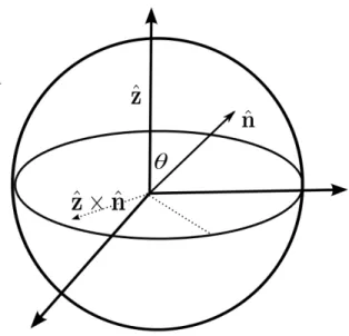
Figure 2.2: The directions of the unit vectors ˆz and ˆn on a two-sphere .
where ˆn = (cos φ sin ✓, sin φ sin ✓, cos ✓) is a unit vector, i.e., ˆn2 = 1, and ˆm = (ˆn⇥
ˆz)/|ˆn⇥ˆz| is a unit vector orthogonal to ˆn, where ˆz is the quantization axis pointing from the origin to the north pole of a unit sphere and ˆn · ˆz = cos ✓ as shown in Fig.(2.2). This state corresponds to a rotation of ˆSz state, i.e., |s, si, to a state with a quantization axis along ˆn on a two-dimensional sphere S2 = SU (2)/U (1). The matrices Ns(ˆn) satisfy the relation
Ns(ˆn
1)Ns(ˆn2) =Ns(ˆn3)e−iG(ˆn1,ˆn2,ˆn3) ˆSz, (2.43)
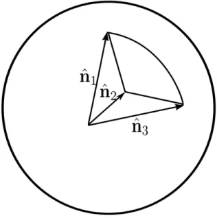
where G(ˆn1, ˆn2, ˆn3) is the area of a spherical triangle with vertices ˆn1,ˆn2, and ˆn3, as
shown in Fig.(2.3). Eqn.(7.50) is however not a group multiplication, thus the matrices
Ns(ˆn)do not form a group representation. Unlike the position and momentum eigen-states in Eqn.(2.5), the inner product of two coherent eigen-states are non-orthogonal:
hˆn0|ˆni = e−isG(ˆn,ˆn0,ˆz)
[1
2(1 + ˆn· ˆn
Figure 2.3: The directions of the unit vectors ˆn1, ˆn2, ˆn3 forming the area of a spherical
triangle.
It has the following property:
ˆ
n· ˆS|ˆni = s |ˆni ) hˆn|ˆS|ˆni = sˆn. (2.45)
The resolution of identity is given by
ˆI = 2s + 1 4⇡
Z
d3ˆnδ(ˆn2− 1) |ˆni hˆn| , (2.46)
where ˆI is a (2s + 1) ⇥ (2s + 1) identity matrix, and the delta function ensures that ˆ
n2 = 1. For any spin Hamiltonian, ˆH(ˆS), the imaginary time propagator can be written
as
23 The derivation of path integral follows as usual by discretizing the time into N slices and inserting the completeness relation Eqn.(2.46). This yields
P(ˆn0, β; ˆn, 0) = Z NY−1 j=1 dχj NY−1 j=0 hˆnj+1|e−✏ ˆH(ˆS)|ˆnji � , (2.48) = Z N−1Y j=1 dχj N−1Y j=0 hˆnj+1|ˆnji − i✏ hˆnj+1| ˆH|ˆnji + O(✏2) � , (2.49) with ˆn0 = ˆnN; ˆn 0 = ˆn; dχj = 2s+14⇡ d3ˆnjδ(ˆn2j − 1). We have that hˆnj+1| ˆH|ˆnji hˆnj+1|ˆnji ⇡ hˆnj| ˆH|ˆnji ; hˆnj+1|ˆnji = e −isG(ˆnj,ˆnj+1,ˆz)[1 2(1 + ˆnj · ˆnj+1)] s.(2.50)
In the continuum limit N ! 1, ✏ ! 0, Eqn.(2.49) becomes [43, 152]
P(ˆn0, β; ˆn, 0) = lim N!1 Z Dˆne−SE(ˆn), (2.51) where SE(ˆn)is given by −SE(ˆn) =−is NX−1 i=0 G(ˆnj, ˆnj+1, ˆz) + s NX−1 i=0 ln ✓ 1 2(1 + ˆnj· ˆnj+1) ◆ − ✏ NX−1 i=0 U (ˆnj), (2.52) where U(ˆnj) =hˆnj| ˆH|ˆnji.
For any closed path on S2, the first term in Eqn.(2.52) which is imaginary is the sum
of the areas of the N contiguous spherical triangles. It leads to the history of the spin trajectory. It is the total area of the topological half-sphere 1
2S
2, with cap ⌃, bounded by
areas differ by 4⇡, i.e.
A(⌃+) = 4⇡− A(⌃−) = lim N!1 N−1X j=0 G(ˆnj, ˆnj+1, ˆz), (2.53) = Z 1 2S2 d⌧ d⇠ ˆn(⌧, ⇠)· [@⌧ˆn(⌧, ⇠)⇥ @⇠ˆn(⌧, ⇠)]⌘ SW Z, (2.54)
This term is called the Wess-Zumino (WZ) action [43, 44, 100, 146, 147]. It is reminis-cent of the Berry phase in condensed matter terminology or the Chern-Simons term in high energy physics. ˆn(⌧) has been extended over a topological half-sphere 1
2S
2 in the
variables ⌧, ⇠. In the topological half-sphere we define ˆn with the boundary conditions
ˆ
n(⌧, 0) = ˆn(⌧ ); ˆn(⌧, 1) = ˆz; (2.55)
so that the original configuration lies at the equator and the point ⇠ = 1 is topologically compactified by the boundary condition. This can be easily obtained by imagining that the original closed loop ˆn(⌧) at ⇠ = 0 is simply pushed up along the meridians to ˆ
n(⌧ ) = ˆzat ⇠ = 1. The Wess-Zumino term SW Z originates from the non-orthogonality of spin coherent states in Eqn.(2.44). Geometrically, it defines the area of the closed loop on the spin space, defined by the nominally periodic, original configuration ˆn(⌧). The ambiguity of modulo 4⇡ in Eqn.(2.53), which corresponds to different ways of pushing the original configuration up, can give different values for the area enclosed by the closed loop as one can imagine that the closed loop englobes the whole two sphere any integer number of times, but this ambiguity has no physical significance since ei4⇡s = 1 for integer and half-odd integer s. Consequently, in the continuum limit, the action becomes
SE[ˆn] = isSW Z + Z
d⌧ U (ˆn(⌧ )); U (ˆn(⌧ )) =hˆn| ˆH|ˆni ; (2.56)
where the Wess-Zumino (WZ) action, SW Zis given by Eqn.(2.54)1. The action, Eqn.(2.56) 1An alternative way of deriving this equation can be found in [15].
25 is valid for semiclassical spin systems whose phase space is S2. It is the starting point
for studying macroscopic quantum spin tunneling between the minima of the energy
U (ˆn).
2.3.2 Coordinate dependent form
Most often a coordinate dependent version of Eqn.(2.56) is used in condensed mat-ter limat-teratures. In this section we will show how one can use any coordinate system of interest. In subsequent chapters, we will show that the coordinate independent form can, indeed, replicate all the known results in quantum spin tunneling. Since the spin particle lives on a two-sphere, the most convenient choice of coordinate are spheri-cal polar coordinates. The unit vector in these coordinates can be parameterize as ˆ
n(⌧, ⇠) = (cos φ(⌧ ) sin ✓⇠(⌧ ), sin φ(⌧ ) sin ✓⇠(⌧ ), cos ✓⇠(⌧ )), with ✓⇠(⌧ ) = (1− ⇠)✓(⌧), which satisfies the boundary conditions, Eqn.(2.55) at ⇠ = 0 and ⇠ = 1. Then
@⌧n = ˆˆ ✓ ˙✓⇠(⌧ ) + ˆφ sin ✓⇠(⌧ ) ˙φ(⌧ ), (2.57)
and
@⇠ˆn = ˆ✓(−✓(⌧)), (2.58)
where ˆ✓ and ˆφare the usual polar and azimuthal unit vectors which form an orthogonal
triad with ˆn such that ˆ✓⇥ ˆφ = ˆn (and cyclic permutations). Thus, we find the triple product in the WZ term becomes
ˆ
n(⌧, ⇠)· (@⌧ˆn(⌧, ⇠)⇥ @⇠ˆn(⌧, ⇠)) = ˙φ(⌧ )✓(⌧ ) sin ✓⇠(⌧ ). (2.59)
Thus, the WZ term, Eqn.(2.54) simplifies to [68, 103]
SW Z = Z d⌧ Z 1 0 d⇠ ˙φ(⌧ )✓(⌧ ) sin ✓⇠(⌧ ) = Z d⌧ ˙φ(⌧ )(1− cos ✓(⌧)). (2.60)