HAL Id: tel-02145438
https://hal.archives-ouvertes.fr/tel-02145438v2
Submitted on 18 Dec 2019
HAL is a multi-disciplinary open access
archive for the deposit and dissemination of sci-entific research documents, whether they are pub-lished or not. The documents may come from teaching and research institutions in France or
L’archive ouverte pluridisciplinaire HAL, est destinée au dépôt et à la diffusion de documents scientifiques de niveau recherche, publiés ou non, émanant des établissements d’enseignement et de recherche français ou étrangers, des laboratoires
Reachability Analysis and Revision of Dynamics of
Biological Regulatory Networks
Xinwei Chai
To cite this version:
Xinwei Chai. Reachability Analysis and Revision of Dynamics of Biological Regulatory Networks. Bioinformatics [q-bio.QM]. École centrale de Nantes, 2019. English. �NNT : 2019ECDN0014�. �tel-02145438v2�
THÈSE DE DOCTORAT DE
L’ÉCOLE CENTRALE DE NANTES
COMUE UNIVERSITE BRETAGNE LOIRE
Ecole Doctorale N°601
Mathèmatique et Sciences et Technologies de l’Information et de la Communication Spécialité : Informatique
Par
« Xinwei CHAI »
«
Reachability Analysis and Revision of Dynamics of Biological Regulatory Networks»
«Analyse d’accessibilité et révision de la dynamique dans les réseaux de régulations biologiques»
Thèse présentée et soutenue àL’ÉCOLECENTRALE DENANTES, le 24 mai, 2019
Unité de recherche : Laboratoire des Sciences du Numérique de Nantes (LS2N) Rapporteurs avant soutenance :
Gilles Bernot Professeur des universités Université Côte d’Azur, Sophia Antipolis Pascale Le Gall Professeur des universités CentraleSupélec, Gif sur Yvette
Composition du jury :
Président : Béatrice Duval Professeur des universités Université d’Angers
Examinateurs : Gilles Bernot Professeur des universités Université Côte d’Azur, Sophia Antipolis Pascale Le Gall Professeur des universités CentraleSupélec, Gif sur Yvette
Morgan Magnin Professeur des universités École Centrale de Nantes Loïc Paulevé Chargé de recherche Université de Bordeaux Olivier Roux Professeur des universités École Centrale de Nantes Dir de thèse : Olivier Roux Professeur des universités École Centrale de Nantes
A
CKNOWLEDGEMENT
First and foremost, I would like to express my sincere gratitude to my advisors Prof. Olivier ROUX and Prof. Morgan MAGNIN for the continuous support of my Ph.D. study for their patience, ideas and contribution of time. This kind support also came to my personal life which helped me to regain motivation and carry on the research when I encountered at the same time academy and mental difficulties. I especially appreciate their tolerance allowing me to explore on my will even the outcome was not satisfying.
Besides my advisor, I would like to thank the rest of my thesis committee: Prof. Gilles BERNOT, Prof. Pascal LE GALL, Prof Béatrice DUVAL and Dr. Loïc PAULEVÉ, for their patient reading, insightful comments and encouragement, but also for the questions which incented me to widen my research from various perspectives.
My sincere thanks also goes to my kind team members. Dr. Emna BEN ABDAL-LAH, Dr. Maxime FOLSCHETTE, Samuel BUCHET and Dr. Loïc PAULEVÉ provided me an opportunity to work with them even after their graduation. Without their precious but abundant support, it would not be possible for me to conduct this research. I would like to especially acknowledge Tony RIBEIRO Sensei for his kindness, enthusiasm, intensity and genius ideas which redirected and accelerated my Ph.D. study.
I gratefully acknowledge the funding provided by China Scholarship Council (CSC) that made my Ph.D. work possible.
My life in Nantes is enriched by my warm-hearted neighbors Geneviève ROCHE and the family of MARCHAND. Also I thank my friends in École Centrale de Nantes for all the fun we have had in the last four years.
Last but not the least, I would like to thank my family for all their love and encourage-ment. For my parents who raised me with curiosity in science and supported me in all my pursuits. For my uncle who talked with me intimately in my sadness and confusion. For my girlfriend who accompanied me spiritually everyday across the ocean.
Thank you.
Xinwei Chai École Centrale de Nantes May 2019
Contents
1 Introduction 1
1.1 Context and Motivations . . . 1
1.1.1 Models in Computational Biology . . . 2
1.1.2 Classification of Models . . . 2
1.1.3 Model Checking . . . 3
1.1.4 Model Learning . . . 3
1.2 Problem Statement . . . 4
1.3 Contributions . . . 4
1.4 Organization of the Manuscript . . . 5
2 State of the Art 7 2.1 Discrete Modeling Frameworks . . . 9
2.1.1 Regulatory Network . . . 9
2.1.2 Bayesian Network . . . 10
2.1.3 Boolean Network . . . 10
2.1.4 Normal Logic Program (NLP) . . . 12
2.1.5 Process Hitting (PH) . . . 13
2.1.6 Asynchronous Automata Network (AAN) . . . 15
2.2 Semantics of Modelings . . . 15
2.2.1 Synchronicity . . . 15
2.2.2 Asynchronicity . . . 17
2.2.3 Generalized Semantics . . . 18
2.3 Model Checking . . . 18
2.3.1 Exact Model Checkers . . . 19
2.3.2 Static Analyzers . . . 19
2.3.3 Reachability Problem . . . 20
2.4 Model Learning and Model Revision . . . 21
2.4.1 Learning From Interpretation Transitions (LFIT) . . . 22
2.5 R´esum´e . . . 22
3 Refined Reachability Analysis via Heuristics 25 3.1 Background . . . 26
3.2 Asynchronous Binary Automata Network . . . 27
3.2.1 Definitions . . . 27
3.2.2 Simplified Local Causality Graph (SLCG) . . . 31
3.2.3 Conclusiveness . . . 33
3.3 Topological Preprocessing . . . 34
3.3.1 Detection and Removal of Cycles . . . 34
3.3.2 Decomposition of SLCG . . . 36
3.4 Reachability Analysis . . . 36
3.4.1 Reachability via Permutations (PermReach) . . . 37
3.4.2 Reachability via ASP (ASPReach) . . . 40
3.5 Extension to Multi-valued Models . . . 46
3.6 R´esum´e . . . 49
4 Model Inference and Revision 51 4.1 Background . . . 52
4.2 Model Completion via Candidate Regulations . . . 54
4.2.1 Problem Description . . . 55
4.2.2 Cut set . . . 56
4.2.3 Completion Set . . . 59
4.2.4 Completion by Over-Approximation . . . 59
4.2.5 Completion by Under-Approximation . . . 61
4.3 Model Inference via Statistics . . . 64
4.3.1 Preliminaries . . . 64
4.3.2 Partial Correlation . . . 66
4.3.3 Variable Reconstruction . . . 70
4.3.4 Toy Example . . . 71
4.4 Model Revision via Reachability and Interpretation Transi-tions (M2RIT) . . . 74
4.4.1 Learning From Interpretation Transitions (LFIT) . . . 75
4.4.2 Formalization . . . 75
4.4.3 Modeling and Learning of Asynchronous Dynamics . . 76
4.4.4 Revision . . . 79
4.4.5 Toy Example . . . 82
5 Tests and Benchmarks 85
5.1 Comparison of Reachability Analyzers . . . 86
5.1.1 Performance on Computing Power . . . 86
5.1.2 Performance on Conclusiveness . . . 87
5.1.3 Performance on Random Examples . . . 88
5.2 Implementation of CRAC and M2RIT . . . 90
5.2.1 CRAC . . . 90
5.2.2 M2RIT . . . 91
5.3 R´esum´e . . . 92
6 Conclusion and Outlooks 95 6.1 Contributions . . . 96
6.2 Future Work . . . 98
A Representation of Different Models 111 A.1 Transformation from BNs to ABANs . . . 111
B Algorithms 113 C Theorems and Proofs 125 D Pure ASP reachability analyzer 129 D.1 Pure ASP Implementation . . . 129
List of Figures
2.1 Representations of Biological Topology . . . 11
2.2 Process Hitting . . . 14 2.3 Update schemes . . . 16 2.4 Discretization . . . 17 2.5 Static analysis . . . 20 3.1 Example of ABAN . . . 29 3.2 Example of SLCG . . . 32 3.3 Limitation of SLCG 1 . . . 34 3.4 Limitation of SLCG 2 . . . 34 3.5 SLCG with cycles . . . 35 3.6 Removal of cycles . . . 36
3.7 Random choice on OR gates . . . 37
3.8 Ordering in SLCG . . . 38
3.9 Counterexample of PermReach . . . 39
3.10 Counterexample of ASPReach . . . 45
3.11 Restricted AAN and extended SLCG . . . 48
3.12 Counterexample of extended SLCG . . . 48
4.1 Big picture of model inference . . . 53
4.2 Example of cut set . . . 57
4.3 Completion set . . . 59 4.4 Completion by over-approximation . . . 61 4.5 Completion by under-approximation . . . 62 4.6 Operations on SLCG(1) . . . 63 4.7 Operations on SLCG(2) . . . 63 4.8 Operations on SLCG(3) . . . 64
4.9 Workflow of model inference via partial correlation . . . 68
4.10 Variable reconstruction . . . 71
4.12 Toy example of M2RIT . . . 82
5.1 SLCG of λ-phage model . . . 87
5.2 Counterexample of PermReach . . . 88
List of Tables
2.1 Transition interpretation table . . . 16
2.2 Update schemes . . . 19
4.1 Example of cut set . . . 58
4.2 Example of completion set . . . 60
4.3 Time-series data . . . 72
4.4 Change rates derived from time-series data . . . 72
5.1 Comparison of different analyzers . . . 89
Abstract
Concurrent systems have been of interest for decades. With their simple but expressive semantics, concurrent systems become a good choice to fit the data and analyze the underlying mechanics. However, learning and ana-lyzing such concurrent systems are computationally difficult. When dealing with big data sets, the state-of-the-art techniques appear to be insufficient, either in term of efficiency or in term of precision.
In this thesis, we propose a refined modeling framework ABAN (Asyn-chronous Binary Automata Network) and develop reachability analysis tech-niques based on ABAN: PermReach (Reachability via Permutation search) and ASPReach (Reachability via Answer Set Programming). Then we pro-pose two model learning/constructing methods: CRAC (Completion via Reachability And Correlations) and M2RIT (Model Revision via Reacha-bility and Interpretation Transitions) using respectively continuous and dis-crete data to fit the model and using reachability properties to constrain the output models.
Chapter 1 states briefly the background and the contribution of our research.
Chapter 2 introduces the state of the art on modeling frameworks, model checkers, different update schemes of modelings and model learning tech-niques. Some of them are referenced in the following chapters.
Chapter 3 presents our modeling framework and its related reachability analyzers based on static analysis. We focus on the inconclusive cases of pure static analysis and extract the key components preventing from a direct solution. We then apply heuristics on these components, solving them with a limited search to reach a more conclusive result of the reachability problem. Chapter 4 presents the methodology of model learning. Our model learn-ers CRAC and M2RIT perform in fact model selection. They choose a model from the candidates satisfying the provided reachability constraints. How-ever the number of candidate models can be exponential, our model learners can shrink the search space with constraints when generating the models.
Chapter 5 shows some comparative and exploratory tests and their re-sults on the methods presented in Chapter 3 and Chapter 4. PermReach and ASPReach are more efficient than traditional model checkers on the reach-ability analysis and they perform a more conclusive analysis while holding the running time in the same scale as pure static analyzers have.
R´esum´e
Les syst`emes concurrents pr´esentent un int´erˆet depuis des d´ecennies. Avec leur s´emantique simple mais expressive, les syst`emes concurrents deviennent un bon choix pour ajuster les donn´ees et analyser les m´ecanismes sous-jacents. Cependant, l’apprentissage et l’analyse de tels syst`emes concurrents sont difficiles pour ce qui concerne les calculs. Lorsqu’il s’agit de grands ensembles de donn´ees, les techniques les plus r´ecentes semblent insuffisantes, que ce soit en termes d’efficacit´e ou de pr´ecision.
Dans cette th`ese, nous proposons un cadre de mod´elisation raffin´e ABAN (Asynchronous Binary Automata Network) et d´eveloppons des techniques d’analyse d’atteignabilit´e bas´ees sur ABAN: PermReach (Reachability via Permutation search) et ASPReach (Reachability via Answer Set Program-ming). Nous proposons ensuite deux m´ethodes de construction et d’appren-tissage des mod`eles: CRAC (Completion via Reachability And Correlations) et M2RIT (Model Revision via Reachability and Interpretation Transitions) en utilisant respectivement des donn´ees continues et discr`etes pour s’ajuster au mod`ele et des propri´et´es d’accessibilit´e afin de contraindre les mod`eles r´esultants.
Le chapitre 1 d´ecrit bri`evement le contexte et la contribution de nos recherches. Le chapitre 2 pr´esente l’´etat de l’art des mod´elisations, des model checkers, des diff´erentes dynamiques associ´e aux mod`es et les techniques d’apprentissage des mod`eles. Certains d’entre eux sont r´ef´erenc´es dans les chapitres suivants.
Le chapitre 3 pr´esente notre cadre de mod´elisation et ses analyseurs d’accessibilit´e associ´es, qui sont bas´es sur l’analyse statique. Nous nous concentrons sur les cas non concluants d’analyse statique pure et extrayons les composants cl´es empˆechant une solution directe. Nous appliquons ensuite des heuristiques sur ces composants, en les r´esolvant avec une recherche limit´ee pour obtenir un r´esultat plus concluant du probl`eme d’accessibilit´e. Le chapitre 4 pr´esente la m´ethodologie de l’apprentissage par mod`ele. Nos syst`emes de construction de mod`eles par apprentissage CRAC et M2RIT effectuent en fait une s´election des mod`eles. Ils choisissent un mod`ele parmi les candidats qui satisfont `a toutes les contraintes d’accessibilit´e donn´ees. Cependant, le nombre de mod`eles candidats pouvant ˆetre de tr`es grande taille, nos r´eviseurs de mod`eles peuvent r´eduire l’espace de recherche avec des contraintes lors de la g´en´eration des mod`eles.
Le chapitre 5 pr´esente quelques tests comparatifs et exploratoires et leurs r´esultats sur les m´ethodes pr´esent´ees aux chapitres 3 et 4. PermReach et ASPReach sont plus efficaces que les v´erificateurs de mod`ele traditionnels pour l’analyse de l’accessibilit´e. Ils effectuent une analyse plus concluante tout en maintenant la dur´ee de fonctionnement `a la mˆeme ´echelle que les analyseurs statiques purs.
List of symbols
∧ logic AND
∨ logic OR
⊕ logic XOR
|A| the cardinality of set A
[i, j] the interval comprising real numbers x satisfying i ≤ x ≤ j [i; j] the interval comprising integers x satisfying i ≤ x ≤ j Ck
n the k-combination in the set of n elements, Cnk= k!(n−k)!n!
ai automaton a is taking value i
x :: y event x happens just before y in the sequence a.next the successor of a
a.pred the predecessor of a
A → bj condition A allows automaton b to reach qualitative level j
N the set of all natural numbers
¯
Chapter 1
Introduction
In the domain of systems biology, more big data are becoming available with the development of biotechnology. However, extracting information from such big data could be difficult due to its high computational com-plexity and the potential fuzziness of biological systems. Modelings and their related analytic techniques are drawing increasing attention. The dilemma of efficiency and precision always persists.
This thesis is dedicated to attacking this dilemma by proposing our modeling framework and its related dynamic properties analyzers as well as model learning methods.
1.1
Context and Motivations
In the studies of concurrent systems, modeling is an inevitable topic. The modeling frameworks discussed in this thesis are all designed for biological use and some features are drawn from biology but they can be potentially useful in other domains, e.g. robotics, human engineering.
Models are supposed to represent the operations of a real system and help one to access, analyze and control the real system. It is a tool to help people to understand the interaction of the components in real systems and the integral behavior of the systems.
A good model is a model which:
• is consistent with the corresponding real system
The model reproduces certain important behaviors. In the ideal situ-ation, the model bisimulates the real system.
• is observable
To allow one to verify the behaviors, the state (historical, current and future) and the mechanics of the model have to be observable. • allows one to access the I/O of the model
With full control of the I/O, we can carry some unfeasible tests in real system as the mechanical of the model is known.
• has related analyzers of various properties
Some properties are not verifiable via finite enumeration. • can be translated from/to other models
Normally, the above metrics are self-constrained: The finer the model is, the bigger the computational complexity is (simulation, verification, etc.). In this thesis, we focus on modelings, their related analyzers of system prop-erties and model revision based on these propprop-erties.
1.1.1 Models in Computational Biology
Systems biologists are interested in highly abstracted models because they need abstract representation and/or flexibility to make model compatible with unknown biological knowledge.
Tractability with big data is also important. “Big” refers to two mean-ings: one is that biological systems can be huge, with enormous number of components and interactions in between; another is that the number and the size of data sets can be huge.
To model the real system, we need components to represent genes, RNA messengers, proteins, metabolites, etc. At this stage, we can carry out a first-step abstraction. The synthesis of proteins is under the instruction of RNA messengers which are synthesized according to genes. This linear process allows to compress the three entities into one. Their inner behaviors (e.g. protein phosphorylation, activation/inhibition of genes) are characterized by the values of the associated entities.
1.1.2 Classification of Models
The values in models can be continuous or discrete which differentiate the modeling frameworks.
Continuous values correspond directly to the measurement and can be used in the models based on the family of Ordinary Differential Equation
(ODE), for example Stochastic Differential Equation (SDE), Delay Differ-ential Equation (DDE).
Discrete values come from an approximation from sigmoid function to step functions. Sigmoid function is a monotonic function and its change rate is high around a certain point (Proof in Appendix C). Many biological behaviors are similar with sigmoid functions: certain entity starts to influ-ence the system if its value goes beyond a certain threshold. If the value is far from the threshold, it is either insufficient (low level) or saturated (high level) [42, 81]. This fact inspires scientists to study discrete models. One can encode low level as 0 and high level as 1 or even add additional discrete levels to represent more behaviors.
In the term of concurrency, synchronous models make components to evolve at the same time while asynchronous ones allow at most one com-ponent to evolve at one time. Due to the fuzziness of biological system, asynchronous models are compatible with more configurations of system parameters [6].
However, the compatibility of asynchronous models is also a shortcoming as they explore more state space at each system transition compared with synchronous ones. The exploration of state space leads to so-called state space explosion problem. To deal with such problem, Paulev´e et al. pro-posed the Process Hitting framework and its related static model checker [61] and Folschette et al. proposed Asynchronous Automata Network enriching model semantics [29]. In this thesis, we mainly work on asynchronous discrete models based on the models above.
1.1.3 Model Checking
If one has an existing model, he might want to know what kind of properties this model satisfies, such as fixed points, safety, reachability.
As stated in the beginning of this chapter, verifying such properties in a concurrent system is costly in computation (PSPACE-complete) [35]. We have to make a compromise on either efficiency or precision: exact ana-lyzers are precise but need to traverse big state space; abstract anaana-lyzers solve a simplified version of the original problem so that the solution is not equivalent to the one of the original problem.
1.1.4 Model Learning
Models are built by the biological knowledge, obtained either by certain experiments, either by generalized conclusions from biologists.
Model learning turns the data coming from biological experiment into model parameters, if the modeling framework is given. We will focus on the LFIT-based method (Learning From Interpretation Transition) proposed by Ribeiro et al. [66, 65, 67]. LFIT is a precise learning technique which takes all the inputs into account.
However, model learning is not enough, as we are not sure the resulted models are consistent with empirical conclusions.
1.2
Problem Statement
With the background of model checking and model learning, we can now formulate the two main problems of this thesis:
• How to analyze efficiently (less runtime) and precisely (less false posi-tive/negative rate) the reachability properties within an asynchronous discrete model?
• How to build a model from time-series data such that the model sat-isfies desired reachability properties?
1.3
Contributions
The main contributions corresponding to the problems are the followings: • Development of efficient and precise heuristic reachability analyzers
based on static analysis [12]
• Design of model revisers: using a priori knowledge and reachability properties to revise existing models
This thesis aims at solving the problems in the last sections by refining existing modeling frameworks and learning approaches:
Reachability analyzers
To solve both the state space explosion problem and the unsatisfying precision of pure static analysis, we developed two approaches based on static analysis with different weights on efficiency and precision.
Model Revisers
As far as we know, model revision based on reachability properties has never been considered in the literature. According to the problems of model inference above, we designed two algorithms:
• an algorithm based on learning from raw time-series data
This algorithm uses correlation coefficients to infer the correlations between the change rate of each variable and other variables in order to suggest hypothetical regulations of the system. With the hypothetical regulations and a priori biological knowledge, we can revise incomplete models by adding transitions consistent with the real system.
• an algorithm based on learning from discretized time-series data The learning approach we applied is the one using Inductive Logic Programming [65]. This approach has more strict rule constraints, the model is either consistent with the original time-series data or not. We try to revise the model in order to make it consistent with a priori biological knowledge and the rule constraints at the same time.
1.4
Organization of the Manuscript
Chapter 2 introduces the state of the art on several modeling frameworks, model checkers, different update schemes of modelings and model learn-ing/revision techniques. We are especially interested in Asynchronous Au-tomata Network, reachability analysis and the learning from state transi-tions.
Chapter 3 presents our modeling framework adapted from Automata Network and its relating reachability analyzers based on static analysis. We will focus on the inconclusive cases of pure static analysis and analyze the key components preventing from a direct solution. We then apply some different heuristics on the key components to solve them dynamically in order to reach a conclusive result on the reachability problem.
Chapter 4 presents the methodology of model revision in this thesis and our model revisers mentioned above. These model revisers perform a model selection. They choose a model from the candidates satisfying all the provided constraints. However the number of candidate models can be huge, our model revisers can shrink the search space drastically to obtain a result.
Chapter 5 shows some comparative and exploratory tests and their re-sults on the approaches presented in Chapter 3 and Chapter 4.
Chapter 2
State of the Art
This chapter is dedicated to the introduction of the basic notions of this thesis. Concretely speaking, we are going to present the state of the art constituting of mainly three basic contents:
• Several modeling frameworks, some of which are the ancestors of the new modelings to be used in this thesis and some of which will be used in comparison
• The notion of model-checking and some existing model checkers • Different update schemes of modeling frameworks
• Several model learning/inference techniques
These notions will be helpful for readers to understand our new model-checkers and new model inference approaches.
In computational biology, there are plenty of modeling frameworks suit-ing different needs. Models are a useful tool to represent the abstraction of the real system, as the real system is usually mechanically complicated and not completely known.
From the point of view of data type, models are classified into continuous ones, discrete ones and their combination, hybrid models, where the last one is not the focus of this thesis.
Continuous models are usually derived from real world data, as the data (no matter time-series data or static data) are obtained by measurement and can be used as input without preconditioning. Differential equations models [33, 76, 80] are based on the hypothesis that in biological systems,
the change rate of variables is numerically related to the values of other variables. Differential equations-based models deal with mainly the system dynamics, e.g. biological regulations. Models based on Bayesian probability and Markov chain [39, 45] study static topics, e.g. phylogenetics.
However, the following difficulties usually arise in the analysis of contin-uous models:
• System mechanics is unclear
• System parameters need to be precise which is difficult for biological system
• Solving differential equations numerically is expensive
Unlike straightforward continuous modelings, discrete modelings per-form an abstraction of continuous dynamics and an over-approximation of continuous constraints [6]. Discrete models can be also inferred from discrete data by discretization [24].
On the aspect of dynamics, discrete models have the following update pattern: discrete state1−−−−−−→ discrete state2, where the states corre-conditions spond to the intervals in the continuous models. States here can be quali-tative levels or combinations of qualiquali-tative levels, compensating the impre-cision or the incompleteness of the original system. Conditions here could be either a necessary time delay or a state of the current system, etc.
As to the computation of various properties, discrete transition mod-els generally cost less than continuous dynamical modmod-els. Among discrete models, Boolean Networks [42], Thomas Models [79], Petri nets [63], Process Hitting Framework [59] could more or less avoid these disadvantages when facing the problems related to system evolution.
Hybrid (in the sense of discrete/continuous) models [83, 48, 75] usually behave like continuous models, because in each discrete block, the sub-model also need continuous parameters as continuous models need. Their compu-tational complexities are of the same scale. We are not going to detail hybrid models during this thesis.
Continuity characterizes the evolution pattern of each variable. However, models contain multiple variables. From the point of view on concurrency, models can be classified according to update schemes into mainly three gen-res: synchronous models, asynchronous models and generalized models.
Synchronous update scheme designates that every component will transit simultaneously to one of its possible future states regardless the time needed
for transition or other components. However in real world, constraints al-ways exist. Biologically it is not probable that multiple components in one system change their state simultaneously. This deficiency demands us to consider more update schemes. Detailed discussion is in Section 2.2.
In this chapter, we will first discuss several discrete modeling frameworks and updating schemes, comparing their differences and the possibility of translating from each other. Some of these models will be used in the fol-lowing chapters. Models need related analytic tools, we will then study some model checkers especially those focusing on reachability properties as many other complex properties can be formulated with the help of reachability. At last we will be interested in the model learning and revising techniques which are the key of constructing a model.
2.1
Discrete Modeling Frameworks
Original biological problems are usually difficult to be studied directly due to the uncertainty and the big scale of biological systems. Modeling is a process of abstracting the real system into a more concise and more easily automatized system. To solve a certain problem, an appropriate modeling framework is crucial because different models have different bias from re-ality and have also different advantages in computation, e.g. fixed point, reachability. Here we are going to introduce several most frequenly applied modeling frameworks and analyze their advantages and disadvantages.
2.1.1 Regulatory Network
Regulatory Networks (RN) have characteristics of a static network, rep-resenting the interactions between components [6]. With the analysis of topological features, it can be applied in for example gene expression anal-ysis [74].
Definition 2.1 (Regulatory network (RN)). A regulatory network is a la-beled digraph G = (V, E) where
• each vertex v of V , called variable, is provided with a boundary bv ∈ N
less or equal to the out-degree of v in G.
• each arc u ∈ v of E is labelled with a couple (tuv, αuv) where tuv is
an integer between 1 and bv, called qualitative threshold and where
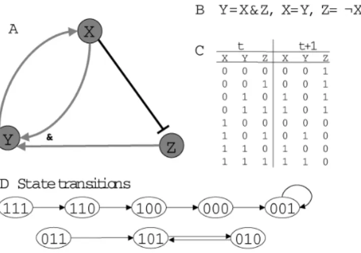
An example is shown in Figure 2.1 A, consisting of three entities X, Y, Z on page 11. Sharp arrows → stand for promotion while blunt arrows a stand for inhibition, e.g. X inhibits Z, Z promotes Y .
RN is a special instance among discrete modelings. It does not require a threshold setting for each variable. As a result, RN is usually applied to study static problems, e.g. model completion, finding fixed points [85]. Without quantitative representation, one can barely analyze the system dy-namics because RN does not possess an update pattern which describes state transitions.
2.1.2 Bayesian Network
Bayesian networks are a type of probabilistic graphical models. They rep-resent joint probability distribution of a set of variables. More concretely, if one obtains the value of certain variable, a Bayesian network can help him analyze the values of its linked variables.
Bayesian networks are usually used for inferring causal dependencies between genes in gene regulatory networks with the goal of estimating the posterior probability of chosen features being inherent in the network, given the data [30].
A Bayesian network is defined as (G, θ) where G is a directed acyclic graph whose vertices connect the random variables of the network. θ is a probability distribution associated to the vertices. These variables can be continuous or discrete. Directed edges correspond to dependencies between variables. θ describes a conditional distribution for each variable of the network, given its “parents” as defined by the relations in G.
One disadvantage of Bayesian networks is that they can only represent acyclic topology as they must be acyclic in order to guarantee that their underlying probability distribution is normalized to 1. However feedback loops appear very frequently in biology which narrow the application of Bayesian networks.
2.1.3 Boolean Network
Boolean Networks (BN) are a traditional framework studied for decades [42]. They discretize every variable of the system into Boolean variables taking values 0 or 1, presenting active/inactive, high/low concentration, etc. Tran-sitions in BNs are defined by Boolean functions. Here we introduce the basic definition of BN.
Definition 2.2 (Boolean Network (BN)). A Boolean Network G(V, F ) con-sists of a set of nodes V = {v1, · · · , vn} and a set of Boolean functions
F = {f1, · · · , fn} where function fi decides the value of node vi of the next
time point: vi(t + 1) = fi(v1(t), · · · , vn(t)).
In some applications, the nodes are classified into incoming nodes, out-going nodes and inner nodes to represent an input-output system [3].
Figure 2.1: Four ways of representing biological topology: A. regulatory network, B. Boolean functions, C. transition interpretation table, D. State transition graph
Figure 2.1 shows different representations of biological topology. RN (A) shows only a qualitative inference graph. BN (B) is concise but does not indicate directly the state change between moments t and t + 1. Its update scheme needs to be precised (in Section 2.2). Transition interpretation table (C) and state transition graph (D) are straightforward but there are two drawbacks:
• the state space increases exponentially with the number of variables leading to the lack of memory
• they are not equivalent to Boolean functions
One set of transition interpretations or one state transition graph could correspond to multiple set of Boolean functions.
In term of expressiveness, BNs can be translated to Normal Logic Pro-grams (NLP) [41]. NLP provides a more dynamical representation and also
for applying SAT techniques in the computation of point attractors of both synchronous and asynchronous semantics [25, 36].
2.1.4 Normal Logic Program (NLP)
Logic programming is a type of programming paradigm which is largely based on formal logic. Any program written in a logic programming lan-guage is a set of sentences in logical form, expressing facts and rules about some problem domain. Major logic programming language families include Prolog, Answer set programming (ASP, which we will detail in Section 3.4.2 of Chapter 3) and Datalog.
In all of these languages, the basic element is called an atom, representing a variable with certain value. The set of atom is denoted B. Rules are written in the form of clauses consisting of atoms (formula representation on the left while code representation on the right):
H ← B1∧ . . . ∧ Bn. or H :- B1, ... , Bn.
H, B1, . . . , Bnare atoms. The rule is read declaratively as logical
impli-cations:
H if B1 and . . . and Bn.
H is called the head of rule and B1, ∧ . . . ∧ Bn is called the body of rule.
Facts are rules having no body, and are written in the simplified form: H.
Using this notation, one can describe the transition of variable: varval0
0 (t + 1) ← var val1
1 (t) ∧ . . . ∧ varvaln n(t).
which reads variable var0 will take value val0 at the next time point if
variable var1takes value val1and . . . and variable varnis taking value valn.
In this thesis we simplify the notation as varval0
0 ← var
val1
1 ∧ . . . ∧ varnvaln.
Remark 2.1. NLP appears to have almost the same formula as BN ac-cording to Inoue et al. [41], the only difference is ← of NLP and = of BN. However, logic OR is not allowed in NLP. The way to represent logic OR is to use additional rules. For example, Boolean function Z = X ∨ Y can be
translated to the following rules: Z1 ← X1, Z1 ← Y1 and Z0 ← X0∧ Y0.
This translation may create non-equivalence and non-determinism. Detailed applications are in Section 4.4.1 of Chapter 4.
2.1.5 Process Hitting (PH)
If one wants to describes the dynamics more finely with reasonable memory use, Process Hitting (PH) framework is a good choice, which was introduced by Paulev´e et al. [59].
PH is inspired by π-calculus, which expresses the communication be-tween canals. In PH, the corresponding meaning becomes the interaction between different components. Process Hitting is an asynchronous automata network, i.e. allowing at most one transition fired simultaneously. PH is more expressive than Asynchronous Thomas’ model [79] or Asynchronous BN [32]. Actions in Process Hitting are more capable of describing various transitions than Boolean functions or attractors as it specifies the regulating and regulated components and their quantitative levels. Also it expresses ex-plicitly the cooperation between several components and stochastic features using π-calculus which are not detailed in this thesis [58].
Moreover, in order to define efficient analysis techniques that avoid to build the whole state space of the model causing state space explosion (in Thomas’ model and Boolean network), various abstract structures have been introduced, and one of them is graph of causality, which allows a reasoning of the reachability of local states instead of traverse of global states.
It gathers a finite number of concurrent processes grouped into a finite set of sorts. A process belongs to one and only one sort and is denoted as ai where a is the sort and i the identifier of the process within the sort a.
At any time, only one process of each sort is present, forming a global state of the PH.
Definition 2.3 (Process Hitting (PH)). A P H consists of a tuple (Σ, L, H): • Σ = {a, b, ...} is the finite set of sorts
• L =Q
a∈ΣLa is the set of states with La = {a0, ..., ala} the finite and countable set of states of sort a ∈ Σ and la a positive integer with:
a 6= b → ∀(ai, bj) ∈ La× Lb, ai 6= bj
• H = {h = ai → bj bk | (a, b) ∈ Σ2, (a
i, bj, bk) ∈ La× Lb× Lb, bj 6=
bk, a = b → ai = bj} is the finite set of actions, which defines the
regulations and dynamics of the PH: ai, bj, bk are denoted hitter(h),
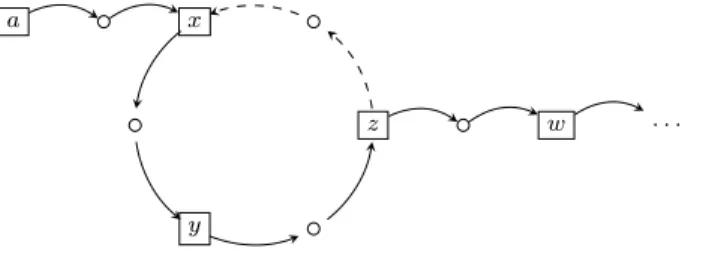
Example 2.1. Figure 2.2 shows a PH P H = (Σ, L, H) constituting of four sorts Σ = {a, b, c, d}, and the possible states of each sort are La= {a0, a1},
Lb= {b0, b1, b2}, Lc= {c0, c1}, Ld= {d0, d1, d2}. The initial state of P H is
α = ha1, b0, c0, d1i. It has actions H = {a0 → c0 c1, a1 → b1 b0, c1 →
b0 b1, b1 → a0 a1, b0 → d0 d1, d1 → b0 b2, c1 → d1 d0}. For
example a0 → c0 c1 means if sort a is at level 0, it allows sort c to jump
from level 0 to level 1.
a 0 1 b 0 1 2 d 0 1 2 c 0 1
Figure 2.2: Gray circles represent the initial state of sorts. Full arrows are regulations while the following dashed arrows are the actions under the condition of the corresponding regulations.
Nevertheless, PH cannot encode equivalently the conjunctions in Boolean functions like f (a) = b ∧ c.
To overcome this drawback, it is needed to introduce a cooperative sort bc to represent the conjunction of b and c, with 8 actions b0 → bc10 bc00,
b0 → bc11 bc01, b1 → bc00 bc10, b1 → bc01 bc11, c0 → bc01 bc00,
c0→ bc11 bc10, c1→ bc00 bc01, c0→ bc10 bc11.
However, the size of this representation grows exponentially with the size of the conjunction and the behavior of cooperative sorts are not equivalent to that of BN. Also, this encoding introduces extra reactions, producing a temporal shift between the presence of the reactants and the playability of the reaction.
2.1.6 Asynchronous Automata Network (AAN)
Facing the drawback of PH, i.e. only cooperative sorts can encode reactions with conjunctions in the hitters, Asynchronous Automata Network (AAN) is introduced by Folschette et al. [29]. AAN allows one to naturally model cooperations by defining several requisites for a transition. Moreover, such automata networks are still compatible with the notion of priority, that can also be used to model different reaction rates in the model. AAN (and, a fortiori, their restriction, the PH framework) can be considered as a subset of Communicating Finite State Machines or safe Petri Nets [60].
Basically the main difference between PH and AAN is state below. Sorts in PH are called automata in AAN. Also, the definition of H becomes
• H = {A → bj bk| b ∈ Σ ∧ (bj, bk) ∈ Lb× Lb∧ bj 6= bk∧ ∀a ∈ Σ, |A ∩
La| ≤ 1 ∧ A ∩ Lb = ∅} is the finite set of actions, which defines the
regulations and dynamics of the AAN: A, bj, bk are denoted hitter(h),
target(h) and bounce(h) respectively of the action h = A → bj bk.
where the action conditions are no longer limited to the state of only one automaton. With the new definition of H, we can now define actions needing multiple local states as condition.
In Chapter 3, we will make use of the definition of AAN by limiting the variables from multi-value ones to Boolean ones in order to obtain some interesting properties in the forthcoming reachability analysis.
2.2
Semantics of Modelings
For a given modeling framework, even if the components and transitions are defined, the dynamics of the system is not unique. Different update schemes lead to different dynamics. The main difference lies on the relations of the number of transitions that can be fired and the number of transitions that will be fired at given time point t [65, 14].
2.2.1 Synchronicity
Literally, synchronous update scheme implies that all fireable transitions are fired simultaneously.
Example 2.2. Taking the transition interpretation table in Table 2.1 as the given system dynamics, Figure 2.3 (a) shows the synchronous case.
t t + 1 u v u v 0 0 2 0 1 0 2 1 2 0 2 1 0 1 0 0 1 1 0 1 2 1 2 1
Table 2.1: Exemplary transition interpretation table indicating the tendency of system evolution from one state to another.
Synchronous update scheme seems to be deterministic. However, when there are multiple fireable transitions available for one variable, there are multiple possible future states which cannot be fired simultaneously. Example 2.3. Given an NLP with rules var13 ← var1
1 and var23 ← var21and
initial state hvar1
1, var12, var30i, these two rules are in conflict. Even though
the semantics is synchronous, a choice is need to be made between these transitions to decide the next state of var3 is 1 or 2.
To avoid the conflicts in Example 2.3, one possible solution in Boolean NLP is to clarify the state transition metrics: for one variable, if it can change its value at the next time point, it cannot keep its current value the NLP is Boolean, there is only one choice for it.
On the computational aspect, one of the benefits of the synchronous model is tractability, while classical state space exploration algorithms fail if there are multiple possible future states at each state transition.
u v
0 1 2 0
1
(a) Synchronous semantics
u v 0 1 2 0 1 (b) Asynchronous semantics u v 0 1 2 0 1 (c) Generalized semantics
2.2.2 Asynchronicity
For biological applications, asynchronous semantics is said to capture more realistic behaviors: at a given time, a single gene can change its expres-sion level. However, these rich behaviors result in a potential combinatorial explosion of the number of reachable states.
Example 2.4. Let us take the same transition interpretation table as Ex-ample 2.3, due to the limit of number of variables which can change their values, the asynchronous case is shown in Figure 2.3 (b).
Given BN with n variables, from a certain state, for deterministic syn-chronous semantic, there is only one path to be exploited. However, for asynchronous semantic, there are at most n future states, after t step of evolution, there are O(nt) possible branches in the arborescent searching
graph which leads to state space explosion problem.
Another problem of asynchronous update scheme is the compatibility with time series data. One cannot guarantee when timeline is discretized evenly whether data of adjacent time points have at most one state transi-tion. Our solution is to discretize timeline according to the moments when variables change their qualitative levels.
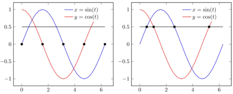
Example 2.5. In Figure 2.4, let us consider a dense enough time-series data (quasi-continuous) with two variables x = cos(t) and y = sin(t). The thresh-olds for both variables are set to 0.5. The left diagram shows equi-temporal discretization of step size 0.5π, while the right diagram discrete time at the moment when x and y reach the threshold, i.e. π/6, π/3, 5π/6, 5π/3. The latter discretization has no conflict with asynchronous update scheme, as there are at most one variable changing its value at each time point.
0 2 4 6 −1 −0.5 0 0.5 1 x = sin(t) y = cos(t) 0 2 4 6 −1 −0.5 0 0.5 1 x = sin(t) y = cos(t)
This PhD thesis focuses on the study of reachability of asynchronous modeling frameworks. We will still introduce in the last part of this section, a more global semantics.
2.2.3 Generalized Semantics
Generalized semantics is even more complex than asynchronous semantics. At any given time, the system can change the values of any number of variables. Given a BN and a current state, if there are m variables which may change their value at the next time point, there will be 2m possibilities of the next state. Generalized semantics contains synchronous and asynchronous semantics.
Example 2.6. Let us take the same transition interpretation table as Ex-ample 2.3, we can update any number of variables at each time point. The generalized case is shown in Figure 2.3 (c).
To sum up, Table 2.2 shows the difference of those three update schemes. For synchronous update scheme, m is the number of different variables in all the heads of rule. The formal definition m is as follows: let R be the set of rules and current state be S = hvarval0
0 , · · · , varnvalni. V = {head(r) |
∃r ∈ R, body(r) ⊆ S}, then m = |V |.
For synchronous cases we can consider the possible future states is of O(1) as it is little probable that many rules are in conflict even though one can create an extreme counterexample making the number of possible future states reach its theoretical limit O(3m) if the number of total states of all the variables is fixed (the proof is given in Appendix C). The possible future states is polynomial for asynchronous cases. However generalized update scheme has to consider the combinatorial results of the fireable transitions. As to asynchronous case, there can be no fireable transitions where n = 0. Hence, the number of transitions will be fired is min(1, n).
The benchmark part of [65] shows the complexity of generalized seman-tics, where the model inference fails with 12 components in the model.
2.3
Model Checking
Model Checking is an automatic verification technique for large state transi-tion systems and was independently developed by Clarke and Emerson [19] and by Queille and Sifakis [64] in the early 1980s. It was originally de-veloped for reasoning about finite-state concurrent systems. Typically, a
Synchronous Asynchronous Generalized nb of fireable transitions n
nb of transitions will be fired m min(1, n) [0; m] nb of possible future states at most O(3m) m [2m; 2n] Table 2.2: Numbers of fireable transitions in different updating scheme, where m stands for the number of different variables in all the heads of fireable transitions.
model checker has three basic components: a modeling formalism adopted to encode a state machine representing the system to be verified, a specifi-cation language based on Temporal Logic, and a verifispecifi-cation algorithm [20] which employs an exhaustive searching of the entire state space to determine whether the specification holds or not.
In this thesis we focus on reachability (EF in Temporal Logic) as most temporal properties can be reduced to reachability problems due to the expressiveness of hybrid modeling frameworks.
2.3.1 Exact Model Checkers
At first, Model Checking was done by the search in the state transition graphs, which are encoded in adjacent lists [19]. This representation however requires a memory growing exponentially with the number of components. To avoid such explicit representation, state transition graphs were replaced by Boolean formulas. OBDD-based (Ordinary Binary Decision Diagram) Model Checkers were developed, having reached 10120states, e.g. SMV [51],
NuSMV [16], and VIS [9]. However, the performance is still not enough to analyze problems in systems biology due to their complexity (PSPACE-complete) [35]. The tests are illustrated in Chapter 5.
2.3.2 Static Analyzers
Model Checkers are widely applied to hardware and software. Especially when applied to software, algorithmic verification techniques have to deal with infinite state space of software, requiring abstraction techniques to make problems tractable. SPIN [38] and Goanna [27] are designed as source code analyzers, by verifying a set of over-approximate conditions, they man-aged to check the safety/liveness properties of a program or whether certain program behaves as expected. However, the static code analyzers only de-termine run-time properties of programs by examining the code structure, which may produce false-positive and false-negative results [82].
Inspired by these ideas, Pint [55] takes the initiative to apply pure static analysis, combine over-approximation and under-approximation [61] to squeeze the state space in order to try to solve the original reachabil-ity problem of a PH or an AAN (See Figure 2.5). Similarly, due to the approximations, the result of Pint is not necessarily conclusive [29].
Under-approximation
Over-approximation
Real dynamics
Figure 2.5: Schema of real dynamics and over-approximation and under-approximation in Pint
2.3.3 Reachability Problem
In the domain of model checking, reachability has been of great interest for over 30 years [18, 20]. Various modeling frameworks and semantics in bioinformatics have been studied: Boolean network [3], Petri nets [50, 26], timed-automata [21, 84]. These approaches rely on global search and thus face state explosion problem as the state space grows exponentially with the number of variables. In [62], it has been shown that the reachability prob-lem of Petri net is exponential time-hard and exponential space-hard, and this conclusion does not change even under some specific conditions [26]. For 1-safe Petri nets, the complexity of reachability analysis is generally PSPACE-complete [15]. Li et al. [46, 47] investigated theoretically the sta-bility, the controllability and the reachability of Switched Boolean Networks, but their method remains computationally expensive; Saadatpour et al. [70] researched only the reachability of fixed points.
To tackle the complexity issue, symbolic model checking [10] based on OBDDs and SAT-solvers (satisfiability) [2] have been studied over years, but still fail to analyze big biological systems with more than 1000 variables.
Bounded Model Checking (BMC) [17] is an efficient approach but generally not complete as its searching depth is limited to a given integer k.
Model checking is not only related to the verification of models, it can be of help to the learning of model and modification according to the unsatisfied properties.
2.4
Model Learning and Model Revision
All the modeling frameworks and model-checkers mentioned above are not effective unless they are fed with trustworthy system topology. Model learn-ing is used to classify the original data into generalized topological knowledge of the system where the original data come from raw data after being dis-cretized, normalized, denoised etc. In this thesis we do not assess the quality of raw data as it is related to the results of biological experiments.
Among the important contributions, Khalis et al. [43] have studied pa-rameter learning in a given model topology. Rodrigues et al. [69] have stud-ied active learning of relational action model whose dynamics is however not compatible with BRNs. Bonneau et al. [7] have developed a learning algorithm based on regression but with the limit on the size of clusters. Opgen-Rhein et al. [54] have studied the learning using correlation coeffi-cients, but their resulting regulatory networks are undirected. Ribeiro et al. have designed LFIT-based (Learning From Interpretation Transitions) learning methods [66, 65, 67] but these approaches cannot deal with noisy or imprecise inputs as all the errors are taken into account during the learning phase.
However, the sensitivity of LFIT can be of benefit in model revision. The choices of revised models are often combinatorial w.r.t the satisfiabil-ity of certain dynamic properties. If we consider another constraint that the revised model has to reproduce exactly the input time-series data, the number of consistent revised models will decrease. Here we introduce some basic ideas of LFIT which will be of help in Chapter 4.
As for model revision, to our knowledge, model revision based on reach-ability properties has never been considered in the literature. One possible related work is cut set [57] to be introduced after LFIT. Cut set is used to detect the atoms cutting critical paths from the initial state and the desired states. By inhibiting these elements, we can ensure the unreachability of the desired states. In practice, cut sets are useful for proposing potential therapeutic targets that have been formally identified from the model for preventing the activation of a particular molecule. However, cut sets are not
of direct help in model revision, as they inhibit certain atoms to be reached rather than modifying the system topology.
2.4.1 Learning From Interpretation Transitions (LFIT)
Ribeiro et al. [66] have designed LFIT aiming at learning a logic program P (definition in Section 2.1.4 on page 12) from a set of state transitions E in the form S1 → S2 where S1, S2 are the states of the system. E can
be extracted from discretized time-series data. Here LFIT considers only synchronous updating scheme, hence we name it as “synchronous LFIT”.
Basically, the mechanics of synchronous LFIT is as follows: it starts from the most general logic program. It verifies whether every element in E is consistent with P . Obtained inconsistencies are classified as conflicts. Then LFIT tries to specialize the conflicting rules by adding atoms in their body to make them harder to be matched. When there is no conflict, P can reproduce perfectly all the state transitions in E.
Algorithm 2 in Appendix B describes the details of synchronous LFIT. To prevent potential ambiguities, we denote assignment operation as := instead of ←.
2.4.2 Cut set
Paulev´e et al. [57] have designed an algorithm for identifying sets of atoms whose activity is necessary for the reachability of a given local state. If all the atoms from such a set are disabled in the model, the concerned reachability is impossible. Those sets are referred to as cut sets and are computed from a particular abstract causality structure, so-called Local Causality Graph (detailed in Section 3.2.2). Via such manipulation on atoms, one may control certain dynamical properties of a BRN.
However, we are going to try to control the systems dynamics by revising the transition rules of a model instead of inhibiting/imposing certain atoms. This need urges us to make modifications on the elements to be inhibited. The detail of cut sets is in Section 4.2.2.
2.5
R´
esum´
e
In this chapter, we presented mainly four main basic contents of the state of the art:
• Update schemes of models
• Model checking and model checkers • Model learning/inference techniques
Modeling frameworks allow one to encode real biological regulatory sys-tems into computable models according to his need (completion, static anal-ysis, dynamic analanal-ysis, simulation etc.). In the next chapter, we will focus on a finer reachability analysis. To achieve this goal, we will propose a new modeling framework ABAN based on existing ones presented in this chap-ter. Also, to better position our new modeling framework and define its dynamics, we introduced different update schemes of models. To validate and evaluate our work (in Chapter 5), we introduced here several represen-tative model checkers to be used for comparison. With the help of model learning technique LFIT and our reachability analysis methods, we managed to develop a model revision method based on desired reachability properties which has never been consider before.
Chapter 3
Refined Reachability
Analysis via Heuristics
Several modeling frameworks and model checking techniques were intro-duced in Chapter 2. We noticed that even though there exist already exact model checkers and static analyzers for reachability problems, they are not sufficient. Exact model checkers always face the state space explo-sion problem when analyzing large models (with more than 50 variables); Static analyzer PINT, designed for Process Hitting/Automata Network is however, theoretically inconclusive, i.e. not able to provide a global solution to arbitrary input. This chapter is going to deepen into the reachability problem for Asynchronous Binary Automata Network via the following steps:
• Why the inconclusiveness problem arises in static analysis methods • What are the problematic topological structures in static analysis • How to deal with such topological structures
As a result, we try to recover the consequence of the information lost due to non-exhaustive search of static analysis and construct a more close approximation of the real dynamics in order to gain a better conclusive-ness.
The contribution of this chapter was published and presented at SASB 2018 in Freiburg, Germany [12].
framework studied in this thesis, Asynchronous Binary Automata Network (ABAN) and the related static analyzer we have specifically designed, Sim-plified Local Causality Graph (SLCG). These two new definitions based on the one of Automata Network in order to adapt to our new reachability analyzers.
Also, to deal with the inconclusiveness problem persisting in previous work [29], we propose at first doing some preprocessings by simplifying the topology of the models in order to try to remove the parts leading to in-conclusiveness. Then we will introduce two new analyzers (PermReach and ASPReach) based on over-approximation. They perform different heuristics, trying to avoid most of the inconclusiveness due to pure static analysis.
3.1
Background
Reachability problem on formal models is a critical challenge where both validation problems (whether the model satisfies the a priori knowledge) and prediction problems (properties to be discovered) meet. From a formal point of view, numerous biological properties in computational models can be transformed to reachability properties. For example, the reachability of state 0/1 of a variable could represent the activation/inhibition of certain gene or synthesis of a protein, while initial state could represent initial observation in an experiment. If the reachability of a certain state contradicts with a priori knowledge, one can modify the model and/or design a new experiment to verify whether there are erroneous information in the a priori knowledge or imprecision in the former observations. Also, reachability analysis is of help to medicine design: for example if one wants to prevent the carcinogenesis of a cell (target state), one possible solution is to find the critical pathways towards the target state and design a medicine to cut them in order to keep the cell healthy.
To tackle the complexity issue, symbolic model checking [10] based on or-dered binary decision diagrams (OBDDs) [34] and that based on SAT-solvers (satisfiability) [2] have been studied over years, but still fail to analyze big biological systems with more than 1000 variables. Bounded Model Check-ing (BMC) [17] is a state-of-the-art approach, it is efficient but generally not complete as its searching depth is limited to a given integer k. One has no idea whether there exists a solution beyond step k or not.
Beside these approaches, abstraction is an efficient strategy to deal with such models of big scale. It aims at approximating the model while keeping the most important parts influencing the reachability. Abstract approaches
often have better time-memory performance but with a loss of information. They solve usually a simplified version of the original model, i.e. the results from these approaches are not necessarily compatible with all the properties of the original model. While studying reachability problems, the system dynamics is abstracted to static causalities between states and transitions.
However, like BMC, abstract approaches do not solve all the instances. In fact, they solve a simplified version instead of the original reachability problem. If the result of the simplified version is not sufficient to imply the one of the original problem, abstract approaches fail (inconclusive). In the following, we are going to formally define the reachability problem and discuss what are the causes of the inconclusiveness and how to solve them.
3.2
Asynchronous Binary Automata Network
In [29], Paulev´e et al. have worked on the modeling of concurrent systems by Asynchronous Automata Network (AAN) and they invented Local causality graph (LCG) [56, 29, 59] to analyze the reachability of AAN. This interpre-tation drastically reduces the searching state-space thus avoids costly global search [61]. However, this pure static analysis is not complete as there are inconclusive cases which can not be decided reachable or not. LCG can only conclude with the following two constraints:
• With no cycles (Section 3.3.1) • With no AND gates (Section 3.2.3)
We are thus going to refine the reachability analysis to deal with more instances. To attack the inconclusiveness problem, we have designed a new discrete modeling framework for concurrent systems [11]: Asynchronous Bi-nary Automata Network (ABAN). In ABAN, we adapted LCG to SLCG (Simplified LCG) to address reachability problem. This approach refers to a static abstraction of the reachability (with an over-approximation of the real dynamics). In binary situation, the approximation of reachability has some interesting properties simplifying the whole reachability analysis. These properties do not hold in multi-valued models (See Section 3.2.2).
3.2.1 Definitions
• Σ = {a, b, . . .} is the finite set of automata with every automaton having a Boolean state;
• The states of A can then be defined: LS = S
a∈Σ
{a0, a1} is the set of all
local states, L = ×
a∈Σ0{a0, a1} is the set of joint states where Σ
0 ⊆ Σ.
Particularly, if Σ0 = Σ, L is the set of global states.
• T = {A → bi | b ∈ Σ ∧ A ∈ L} is the set of transitions. For transition tr = A → bi, A (called head, noted head(tr)) is the set of required
state(s), which allows to flip b1−i to bi (called body, noted body(tr)).
In other words, transition tr is said fireable iff A ⊆ s, where s is the current global state.
Remark: In AAN and PH, their transitions (or called actions) are noted A → bi bj to express “automaton b changes its value from i to j under
condition A”. However, the states in ABAN are all binary, the transition can only be realized from 0 to 1 or conversely. Thus we omit the state before transition while avoiding ambiguity. It might also be noted the notation A → bi resembles the equivalent notation in Normal Logic Program (NLP):
bi← A.
Also, the notions of different states are crucial in this thesis. A local state represents the state of one automaton, e.g. a1 means automaton a
is at level 1. A joint state represents the state of a set of automata, e.g. ha1, b0i means automaton a is at level 1 and automaton b is at level 0. In
fact, when we take all the automata in the system as the set of automata, the corresponding joint state becomes the state of the whole system, which is the global state, e.g. given Σ = {a, b, c}, ha0, b1, c0i shows the state of
all the automata. To conclude, joint state is the most general case, when |Σ0| = 1, it becomes a local state; when Σ0= Σ, it becomes a global state. Definition 3.2 (Dynamics). From current global state s, the global state after firing transition tr = A → bj is denoted s · tr = s\{bi}∪{bj}, bi∈ s. If
there does not exist fireable transition, s remains unchanged. The state of a certain automaton a is noted (s · tr)[a].
The definition of dynamics allows one to describe how the system state interacts with the transitions. Moreover, to describe the evolution in an ABAN, we use the notion of trajectory.
Definition 3.3 (Trajectory). Given an ABAN A = (Σ, T ) and a global initial state α ∈ L, a trajectory t from α is a sequence of transitions t = tr1::
· · · :: tri :: · · · :: trnwith tri∈ T and each triis fireable in (α · tr1· . . . · tri−1).
From α, the global state after firing all transitions of t is (α · tr1· . . . · trn),
denoted α · t.
A trajectory describe the historical evolution of the system or one possi-ble future evolution by recording the fired transitions. An alternative is to record the state changes using state sequence:
Definition 3.4 (State sequence). Given an ABAN A = (Σ, T ) and a global initial state α ∈ L and trajectory t, the state sequence seq = s1 :: · · · ::
si :: · · · :: sn with si ∈ LS is formed by the updated local states during the
trajectory t.
Thanks to asynchronicity, at each time step ABAN changes the value of at most one automaton. That is why we can distinguish the order of state changes, thus form a state sequence.
Example 3.1 illustrates all the definitions above.
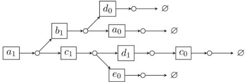
Example 3.1. Figure 3.1 shows an ABAN of 5 automata a, b, c, d, e, with the set of transitions T = {{b1, c1} → a1, {e1} → a1, {d0} → b1, {d1} →
c1, {b1} → d1} and the initial state α = ha0, b0, c0, d0, e0i. A possible
tra-jectory from α is t = {d0} → b1 :: {b1} → d1 :: {d1} → c1 :: {b1, c1} → a1.
After firing the transitions in trajectory t, the global state becomes Ω = s · t = ha1, b1, c1, d1, e0i, and the local state of a is (α · t)[a] = a1. The
corresponding state sequence is seq = b1 :: d1:: c1 :: a1.
a 0 1 b 0 1 c 0 1 d 0 1 e 0 1 {b1, c1} {e1} {d0} {d1} {b1}
Figure 3.1: An example of ABAN
With the definition of trajectory and that of state sequence, we can address reachability problem.
Definition 3.5 (Reachability problem). Given an ABAN, the joint reacha-bility REACH(α, Ω) can be formalized as: joint state Ω is reachable iff there exists a trajectory t s.t. α · t = Ω. Partial reachability reach(α, ω) is defined analogously: local state ω = ai is reachable iff there exists a trajectory t s.t.
(α · t)[a] = ai. REACH(α, Ω) and reach(α, ω) take Boolean values True,
Example 3.2. Taking the same ABAN as in Example 3.1, target global state Ω = ha1, b1, c1, d1, e0i or target local state ω = a1 are reachable from
the initial state α via trajectory t or state sequence s, i.e. reach(α, a1) =
True and REACH(α, Ω) = True.
One can define various dynamical properties by using reachability, e.g. safety (there exists no trajectory from any initial state to an unwanted state), robustness (there exist trajectories from any initial state to a wanted state). Moreover, Proposition 3.1 explains the reachability of a joint state even a global state can be transformed to that of a local state.
Proposition 3.1 (Transformation of reachability). Given an ABAN A = (Σ, T ) and a joint reachability problem REACH(α, Ω), there exists an ABAN A0 = (Σ, T0) with Σ0 = Σ∪{x} and T0 = T ∪{Ω → x1} s.t. the
local reachability problem in A0, reach(α0, x1) with α0 = α∪{x0} is
equiva-lent to REACH(α, Ω) in A.
Proof. If REACH(α, Ω) = True, there must exists a trajectory t satisfying α · t = Ω. t is consistent with A0 with initial state α0 as A0 contains all the elements in A and α ⊂ α0. After firing all the transitions in t, the global state becomes Ω∪{x0}, transition Ω → x1 is fireable and x1 is reachable
from α0 via t0 = t :: Ω → x1, thus reach(α0, x1) = True.
If REACH(α, Ω) = False, there does not exist a trajectory t satisfying α · t = Ω. In A0, this conclusion remains true as the only added transition Ω → x1 is useless in the reachability of Ω. The only pathway towards x1 is
through Ω → x1, as Ω is not reachable, x1 is not reachable, reach(α0, x1) =
False.
Similarly, we can prove the global reachability from local one.
One advantage of ABAN Many biological regulatory networks are en-coded in Boolean style, e.g. in [3, 42], because BN is a simple formalism but with strong applicability: discretization in BN is a way to handle the imprecision of a priori knowledge on the model. However BN may be not expressive enough. If one wants to model the dynamic behavior “a ← 1 at moment t + 1 if b = 1 at moment t”, the translation is a(t + 1) = b(t) in BN. It means a always follows the evolution of b but with a redundant behavior “a ← 0 when b = 0 at moment t” which is not defined in his need. ABAN models this dynamics as {b1} → a1 without this redundancy.
Besides, BNs are transformable to ABANs, and this property makes our approach applicable to a wider domain (Appendix A.1 Translation between Models).