HAL Id: hal-01147312
https://hal.archives-ouvertes.fr/hal-01147312
Submitted on 30 Apr 2015
HAL is a multi-disciplinary open access
archive for the deposit and dissemination of
sci-entific research documents, whether they are
pub-lished or not. The documents may come from
teaching and research institutions in France or
abroad, or from public or private research centers.
L’archive ouverte pluridisciplinaire HAL, est
destinée au dépôt et à la diffusion de documents
scientifiques de niveau recherche, publiés ou non,
émanant des établissements d’enseignement et de
recherche français ou étrangers, des laboratoires
publics ou privés.
MIMO in Home Networks
Khouloud Issiali, Valéry Guillet, Ghaïs El Zein, Gheorghe Zaharia
To cite this version:
Khouloud Issiali, Valéry Guillet, Ghaïs El Zein, Gheorghe Zaharia. Impact of Antennas and Correlated
Propagation Channel on BD Capacity Gain for 802.11ac Multi-User MIMO in Home Networks. The
International Conference on WIreless Technologies embedded and intelligent Systems (WITS 2015),
Apr 2015, Fez, Morocco. �hal-01147312�
WITS-2015
Page 1Impact of Antennas and Correlated Propagation
Channel on BD Capacity Gain for 802.11ac
Multi-User MIMO in Home Networks
Khouloud ISSIALI*, Valéry Guillet**
Engineering and Propagation Department Orange Labs, 1 rue Louis et Maurice De Broglie
90007 Belfort Cedex, France
{khouloud.issiali, valery.guillet}@orange.com
Ghais El Zein+, Gheorghe Zaharia+
+IETR–INSA,
UMR 6164, 20 av. des buttes de Coësmes, CS 70839, 35708 Rennes Cedex 7, France {ghais.el-zein, gheorghe.zaharia}@insa-rennes.fr
Abstract— In this paper, we study the impact of antennas and propagation channel on the block diagonalization (BD) capacity gain for 802.11ac Multi-User MIMO (MU-MIMO) in Home Networks. A correlated channel model is examined. The effect of the number of the transmit antennas, their spacing, and SNR is explored. It is shown that only a small increase of the number of transmit antennas over the total number of spatial streams increases the MU-MIMO capacity gain over SU-MIMO considerably. For example, a gain of 45% is achieved for a 20 dB SNR with 4 spatial streams and 6 transmit antennas. Additionally, the half wavelength antenna spacing is sufficient to take advantage of BD gain and to keep a transmit antenna with compact size. Based on simulations, we reveal the importance of a new channel correlation parameter to explain MU-MIMO capacity gain.
Keywords: MU-MIMO, IEEE 802.11ac, home networks, channel capacity, channel models.
I. INTRODUCTION
In a multi-user downlink scenario, an access point (AP) is equipped with multiple antennas and is simultaneously transmitting several independent spatial streams to a group of users. Each of these users is also equipped with a single or multiple antennas. The management of multiple users generates a new interference called inter-user interference (IUI). Several studies focused on the MU-MIMO solutions to overcome multipath propagation and users’ interference.
In this context, the new standard IEEE 802.11ac ratified in January 2014 normalizes the MU-MIMO processing, namely precoding techniques [1]. The use of these methods aims to increase data rates above 1 Gbps and to improve capacity. The precoding methods can be classified according to several criteria [2]. The classification that has been frequently used is whether the technique is linear or not. We could distinguish then two major classes of precoding, namely non-linear precoding and linear precoding.
Linear precoding techniques have an advantage in terms of computational complexity. Non-linear techniques have a higher computational complexity but can provide better performance than linear techniques. The non-linear techniques are also
known to achieve optimum capacity. In fact, it was proven that the capacity region of the MU-MIMO downlink can be achieved with dirty paper coding (DPC) [3]. The linear method that is most explored in the literature is block diagonalization [4] for downlink MU-MIMO systems. The main principle of BD is to ensure zero inter-user interference as a first step, and then to maximize capacity. Thus, with perfect channel state information (CSI) at the transmitter, BD transforms a MU-MIMO system into several parallel single-user MU-MIMO (SU-MIMO) systems after cancelling the inter-user interference. In fact, when the CSI is provided at the access point, zero inter-user interference is achievable at every receiver, enabling thereby a simple receiver at each user.
The DPC sum capacity gain over BD has been studied in [5]. It was shown that DPC and BD are equivalent for low SNR and a low number of users. Nevertheless, with a high number of users, the DPC gain over BD is considerable.
Most articles on MU-MIMO have studied BD over Rayleigh fading channel [2], [5]. To the best of our knowledge, no article has studied so far the BD performance based on the MU-MIMO correlated channel models defined for 802.11ac (TGac channel models). Furthermore, for this case no study considering the impact of antennas and propagation aspects on BD performance has been done, unlike for 802.11n networks [6]. Also, the case of users with more than a single antenna has been rarely studied [7].
This paper addresses the impact of transmit antennas and propagation on BD performance gain over SU-MIMO in a MU-MIMO downlink. Due to the great success and generalization of Wi-Fi in home networks, a residential environment is considered for this study. To have comparisons with an ideal case, we also study a non-correlated Rayleigh channel. The rest of this paper is organized as follows. Section II describes the system model, presents the block diagonalization algorithm and gives the capacity computation method for MU-MIMO and SU-MIMO systems. Section III presents the MU-MIMO channel model and describes the simulation process. The simulations results are provided in Section IV. Finally, the conclusion is drawn in Section V.
WITS-2015
Page 2 We briefly summarize the notation used throughout thisarticle. Superscript denotes transpose conjugate. Expectation (ensemble averaging) is denoted by E(.). The Frobenius norm of a matrix is written . Finally, the index k is used as a user index throughout this article and it runs from 1 to K, where K is the number of users in the studied system.
II. SYSTEM MODEL,BLOCK DIAGONALIZATION ALGORITHM,
AND RELATED CAPACITY
The studied MU-MIMO system is composed of K users connected to one access point as shown in Fig. 1. The access point has transmit antennas and each user k has
receive antennas. We define ∑ .
Fig. 1. Diagram of MU-MIMO system.
The (where is the number of parallel symbols transmitted simultaneously for the kth user) transmit symbol vector for user k is preprocessed at the access point before being transmitted. The baseband received signal at the kth receiver is given by:
∑
where is an matrix that refers to the MIMO channel matrix for the kth receiver, is the BD precoding matrix intended to the kth user resulting in an
(L = L1 + L2 + … + LK) precoding matrix , is the noise vector composed of complex Gaussian noises ( ).
For the following, we provide a single carrier calculation since the multipath channel is considered to be narrowband for each sub-channel in the OFDM 802.11ac transmitted signals.
Block diagonalization [4] is a transmit preprocessing technique for downlink MU-MIMO systems. BD decomposes the MU-MIMO downlink system into K parallel independent SU-MIMO downlink systems.
The BD method consists first in perfectly suppressing the IUI (IUI =
∑
for each user k, to have parallel SU-MIMO systems. Then, a usual transmit beamforming is applied to optimize the capacity for each user. The precoding matrix is a cascade of two precoding matrices and ,
where is for nullifying the IUI and is for optimizing capacity: = .
The multi-user sum capacity is expressed as follows for each OFDM subcarrier [7]:
∑ ∑
where is the power dedicated to the ith antenna for the kth
user, are the eigenvalues of the effective channel for the kth
user after applying the IUI cancellation, and is the noise power. Note that this article considers an equal repartition of transmit power between spatial streams and subcarriers. The subcarrier index is not mentioned throughout this paper in order to simplify the notations, but since is related to H,
depends on each OFDM subcarrier.
For the corresponding SU-MIMO systems and for relevant comparisons with MU-MIMO, the number of antennas and remains unchanged. The considered SU-MIMO system applies a singular value decomposition and its capacity is
computed as detailed in [8] for each OFDM subcarrier. For SU-MIMO and MU-MIMO systems, the number of the used spatial streams is given by = rank(
The signal to noise ratio (SNR) is defined as , where is the total transmit power. We apply the common normalization | ) which means that the average propagation loss is 0 dB [9].
III. SIMULATION DESCRIPTION AND CHANNEL MODEL
A. Description of the Channel Model
A MIMO channel model was first specified for the 802.11n standard, within the TGn task group [10]. It is based on the cluster model, originally proposed by Saleh and Valenzuela for single-input single-output (SISO) channels [11]. Afterwards, the TGac task group [12] has proposed modifications to the basic TGn model. The modifications concern the Power Angular Spectrum (PAS) to allow MU-MIMO operation and it is summarized as follows [11]:
The defined TGn azimuth spread for each cluster remains the same for all users.
For each user, independent offsets between +/-180° are introduced for the angle of arrival (AoA), for both the direct tap and the NLOS taps.
For each user, independent offsets between +/-30° are introduced for the angle of departure (AoD) for the angle of arrival (AoA), for both the direct tap and the NLOS taps.
Therefore, for MU-MIMO scenarios, channels shall be modeled by randomly drawing for each user these four offset values.
TGn [10] has specified six different channel models (A, B, C, D, E, F) for different environments: office environment (D), large open space and office environments (E)... This paper shows results according to channel model B. This channel model has 9 Rayleigh-fading taps, and each tap has a Bell
WITS-2015
Page 3 Doppler spectrum to consider the random time variability of anindoor channel.
Thereafter, a uniform linear array of antennas at the AP is simulated with the propagation channel model TGac-B (15 ns RMS delay spread) for the 5.25 GHz frequency band. Transmit and receive MIMO channel correlation matrices are modeled through the power angular spectrum.
Rayleigh fading is exhibited for each tap (excepted for the LOS tap which follows a Rice fading with a 0 dB Rician factor), by the assumption that the real and imaginary parts of the taps are modeled by independent and identically distributed (i.i.d.) zero-mean Gaussian processes so that different taps are uncorrelated.
B. Simulation Process
The simulated system is composed of one access point equipped with multiple antennas (linear array of dipole antennas, vertically polarized), and two receivers. Each receiver has two dipole antennas. A Matlab source code [10] was used to compute the different 802.11ac channel samples. As mentioned before, the channel model B has 9 Rayleigh-fading taps. For each tap complex amplitude, the transmit and receive correlation matrices are calculated. The time domain channel was converted to frequency domain by discrete Fourier transform taking into account the characteristics of IEEE 802.11ac.
Block diagonalization method is investigated considering a total transmit power equally shared over all spatial streams.
To have statistical results, 100 couples of users (K = 2) are randomly drawn around the access point. For each drawing, we use a simulation length equal to 55 coherence times of the MIMO channel to simulate the fast fading. By setting the ―Fading Number Of Iterations‖ in the Matlab channel model to 512, 488 interpolated channel samples are collected for each couple of users. The default configuration parameters are summarized as follows:
SNR = 20 dB for all users
Number of spatial streams ( ):
Number of users:
Number of receiving antennas:
Transmit antenna spacing: 0.5λ
Receive antenna spacing: 0.5λ
The residential LOS channel (TGac-B LOS) concerns users in LOS with the access point. The residential NLOS channel (TGac-B NLOS) concerns users in NLOS with the access point. Both TGac-B channel LOS and TGac-B channel NLOS lead to almost the same results. This is because the Rice factor in the TGac-B model is set to 0 dB for the first tap, which is very close to Rayleigh. Hence, in the remainder of this article, we only present the results for TGac-B channel NLOS.
IV. SIMULATION ANALYSIS AND SYSTEM RECOMMENDATIONS In this section, some numerical results are presented. The effect of the propagation channel and transmit antennas (number and spacing of transmit antennas) is analyzed. The impact of SNR is also analyzed. The aim is to assess the weight of each parameter on the BD capacity gain over SU-MIMO and to give recommendations to optimize MU-MIMO performance.
To highlight the BD capacity gain over SU-MIMO, most graphs below show the average of MU to SU capacity ratio. For 2 users, the optimal capacity gain value would be 2.
A. Antenna Spacing Effect
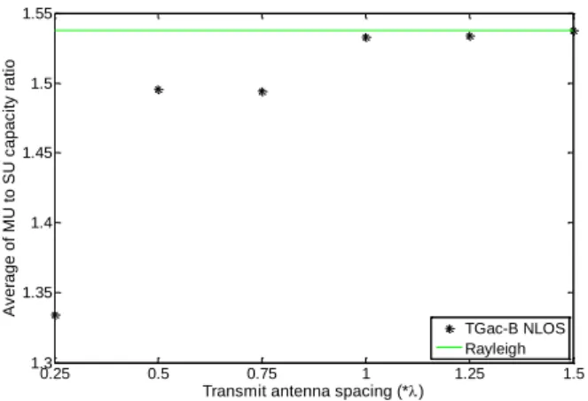
For the following, the number of transmit antennas is fixed to , and SNR = 20 dB. To study the transmit antenna spacing, six values are used: 0.25λ, 0.5λ, 0.75λ, λ, 1.25λ and 1.5λ.
In Fig. 2, the first value (0.25λ) presents an isolated and very low gain (33%) compared to the other spacings. For a transmit antenna spacing of 0.5 λ and above, the capacity gain of MU-MIMO compared to SU-MIMO is around 55% and it almost attains the gain in a Rayleigh channel. Antenna spacing has no effect on the Rayleigh channel since its MU-MIMO channel matrix elements are complex Gaussian and independent. Considering a trade-off between the antenna size and the MU-MIMO capacity gain, the recommendation is to have the antenna spacing equal to 0.5λ. This value is used for the results presented in the remainder of this paper.
Fig. 2. Average of MU to SU capacity ratio versus transmit antenna spacing.
B. SNR Effect
Fig. 3 shows the MU capacity gain over SU versus SNR with 6 transmit antennas spaced 0.5λ in NLOS conditions. For high SNR, MU-MIMO outperforms SU-MIMO in terms of capacity with gain changing from 10% till 70%. Nevertheless, for low SNR, SU-MIMO performs better than MU-MIMO in terms of capacity. It is not practical to have too low SNR for MU-MIMO as it would not be possible to have CSI with no errors to apply the BD precoding.
0.25 0.5 0.75 1 1.25 1.5 1.3 1.35 1.4 1.45 1.5 1.55 A v e ra g e o f M U to S U c a p a c ity r a ti o
Transmit antenna spacing (*)
TGac-B NLOS Rayleigh
WITS-2015
Page 4 The capacity gain is 30% when the SNR increases from 0 to10 dB, or from 10 to 20 dB, or from 20 to 30 dB, and around 10% when it changes from 30 to 40 dB. To conclude about the
SNR, the desired range and the desired bit rate are put forward.
For the following results, a middle case is evaluated with SNR = 20 dB.
Fig. 3. Average of MU to SU capacity ratio versus SNR.
C. Number of Transmit Antennas
Fig. 4 gives the average of MU to SU capacity ratio versus the number of transmit antennas for TGac-B channel NLOS and Rayleigh channel. Average values, 10% and 90% quantiles (q10 and q90) are represented to estimate the confidence
intervals.
The first observation drawn from Fig. 4 is that the MU capacity gain over SU-MIMO increases with the number of transmit antennas. It changes from 1.2 to 1.65 for the residential environment, i.e. around 45% of capacity gain.
We also observe that the gain from 4 to 6 is much higher than the one observed from 6 to 8 or the one observed from 8 to 10. This can be explained by the fact that we cannot take benefit of the transmit beamforming for 4, since the number of transmit antennas is the same as the total number of spatial streams. Another explanation concerning the channel correlation is given hereafter.
Fig. 4. Average of MU to SU capacity ratio versus the number of transmit antennas.
Fig. 5. Capacity value achieved by an i.i.d Rayleigh and TGac-B NLOS channels.
In order to optimize the MU-MIMO capacity gain and have a less congested system, we recommend using 6, when we have a system with two receivers and two antennas each.
Fig. 5 shows the average capacity value for MU-MIMO and SU-MIMO. The capacity value for MU-MIMO increases more rapidly than SU-MIMO. It achieves 27.5 bits/s/Hz versus 16.5 bits/s/Hz for SU-MIMO for 10.
D. Correlation Coefficient
In this section, a correlation parameter is explored as a relevant parameter to explain the previous results concerning and MU-MIMO capacity gain. This parameter is used to analyze the correlation coefficient of the MIMO channels H1 and H2 between the AP and each user. MU-MIMO
channel correlation coefficient was previously studied for the particular case of a single antenna receiver [13].
In the case of a multiple antennas receiver, there is not a single definition of the channel correlation. Theoretical studies comparing BD and DPC have proved, that in the particular case where > , BD achieves the DPC optimal bound if [14]. At the opposite side, is a worst case for MU-MIMO, as BD fails to cancel IUI. Several possibilities exist, but these theoretical results for extreme cases and our simulations revealed that the following definition was the most relevant to explain MU-MIMO capacity gain [15]:
| |
with: ||H1(i,:)||=1, ||H2(j,:)||=1, [ ] and [ ].
Let’s define: (
) and (
) where represents the ith row of the matrix of size .
0 10 20 30 40 0.9 1 1.1 1.2 1.3 1.4 1.5 1.6 1.7 1.8 A ve ra g e o f M U t o S U ca p a ci ty ra ti o SNR (dB) 4 5 6 7 8 9 10 0.9 1 1.1 1.2 1.3 1.4 1.5 1.6 1.7 1.8 M U to S U c a p a c ity r a ti o
Number of transmit antennas Rayleigh (q
90)
TGac-B NLOS (q
90)
Rayleigh (mean) TGac-B NLOS (mean) Rayleigh (q 10) TGac-B NLOS (q10) 4 5 6 7 8 9 10 12 14 16 18 20 22 24 26 28 30 Cha n n e l c a p a c ity i n b its /s /Hz
Number of transmit antennas MU TGac-B NLOS
MU Rayleigh SU TGac-B NLOS SU Rayleigh
WITS-2015
Page 5 The product (
) ( ) is a matrix whose elements are: ( )
. Thus, the
correlation coefficient can be expressed as:
∑ |
|
| | represents the correlation between each single
receiving antenna subsystem of the first user and each single receiving antenna subsystem of the second user. This the more common correlation coefficient used in the case of single antenna receivers. represents an average value of the correlation coefficient between any single antenna receiver subsystem combination.
The average of MU to SU capacity ratio versus the average of the correlation coefficient is presented in Fig.6, for simulations considering . The average is computed here only over time, and each point represents one of the 100 samples of user couples. When the correlation coefficient increases, the capacity gain decreases: more than 30% of capacity loss when the correlation coefficient goes from 0.05 to 0.35. Actually, when both channels (H1 and H2) are correlated,
similar in other words, the BD algorithm does not show great performance. Thus, the gain decreases. It is the case when the two users are close enough. This correlation coefficient has the great advantage of optimizing the users grouping in a MU-MIMO scenario. For example, a system could be optimized by selecting the K users minimizing ∑
|| || .
Fig. 6. Average of MU to SU capacity ratio versus the average correlation coefficient.
The impact of the number of transmit antennas versus average correlation coefficient is presented in Fig. 7. The averaging is performed over all the MU-MIMO channel samples. The average correlation coefficient decreases with the number of transmit antennas. Once more, the two types of residential channel (LOS, NLOS) follow the same trend. The
values are higher but remain relatively close to the ones obtained for Rayleigh channel. We can observe that even if the simulated Rayleigh channel has independent elements in H1
and H2, the average correlation coefficient is not zero,
which is not an intuitive result. Through computation (see Appendix), the average correlation coefficient for an i.i.d MIMO Rayleigh fading channel is proven to be: E( . This result is validated through simulations (Fig. 7).
Fig. 7. Average correlation coefficient versus the number of transmit antennas.
V. CONCLUSION
In this paper, we have investigated the impact of antennas and propagation channel on the block diagonalization (BD) capacity gain for the 802.11ac MU-MIMO in home networks. The obtained results are based on the MU-MIMO correlated channel model specified for 802.11ac for two-antenna user. This article gives recommendations to optimize MU-MIMO capacity in terms of number of transmit antennas, transmit antenna spacing and SNR effect. In particular, we have proved that a small increase of the number of transmit antennas compared to the total number of transmitted spatial streams improves significantly the user channel de-correlation and the MU-MIMO capacity gain over SU-MIMO: for example a gain of 45% is achieved for a 20 dB SNR, 4 spatial streams and 6 transmit antennas. We have also highlighted a relevant channel correlation definition that is useful to decide whether MU-MIMO outperforms SU-MU-MIMO and to select the users into a MU-MIMO user group.
In further work, MU-MIMO measurements will be conducted to compare these results with real propagation channels.
APPENDIX
CORRELATION COEFFICIENT FOR RAYLEIGH FADING CHANNEL
For a MIMO i.i.d Rayleigh fading channel, each element of the channel matrix follows a zero mean complex Gaussian
0.05 0.1 0.15 0.2 0.25 0.3 0.35 0.4 1.3 1.35 1.4 1.45 1.5 1.55 1.6 1.65 A v e ra g e o f M U to S U c a p a c ity r a ti o
Average correlation coefficient
TGac-B LOS TGac-B NLOS 4 5 6 7 8 9 10 0.05 0.1 0.15 0.2 0.25 0.3 A v e ra g e c o rr e la ti o n c o e ffi c ie n t
Number of transmit antennas
TGac-B LOS TGac-B NLOS Rayleigh
WITS-2015
Page 6 process (with the same standard deviation and all theseelements are independent. Let’s define: (
) and (
) where represents the ith row of the matrix .
The complex Gaussian coefficients and , p,q=1... can be written in terms of their amplitudes , , and phases as:
∑
∑
where, , , are independent, , follow a Rayleigh law, and an uniform law in .
The product (
) ( ) is a matrix whose element is: ( )
. We can express as: ∑ (| | )
(| | ) does not depend on the indexes i and j as the
corresponding laws for the elements of the matrix and do not. So we can simplify (6) as:
(|∑ | ) (|∑ √∑ √∑ ( )| )
Then, using the statistical independence of , , , (8) can be simplified as:
∑ (∑ ( )
∑ )
All terms in the sum are identical, so that:
(∑ ( )
∑ )
Because and are independent, we can deduce:
( ( ) ∑ ) ( ( ) ∑ ) Let’s define (∑ ( ) ) We have: (∑ ( ) ) =E( ( ) ) ( ( ) ( ) )
Consequently, the quantity A is: and similarly we have (∑ ( )
) . Finally, E(
REFERENCES
[1] 802.11ac-2013 - IEEE Standard for Information technology-- Telecommunications and information exchange between systems — Local and metropolitan area networks -- Specific requirements -- Part 11: Wireless LAN Medium Access Control (MAC) and Physical Layer (PHY) Specifications -- Amendment 4: Enhancements for Very High Throughput.
[2] A. Lee Swindlehurst, M. Haardt, C. B. Peel, Q. H. Spencer and B. M. Hochwald, ―Space-Time Processing for MIMO Communications‖, (chapter Linear and Dirty-Paper Techniques for the Multi-User MIMO Downlink), 2005.
[3] M. H. M. Costa, ―Writing on dirty paper (corresp.)‖, IEEE
Trans. on Inf. Theory, pp. 439–441, May 1983.
[4] L-U Choi, R.D. Murch, "A transmit preprocessing technique for multiuser MIMO systems using a decomposition approach",
IEEE Trans. on Wireless Comm., vol. 3, no. 1, pp. 20-24, Jan.
2004.
[5] Z. Shen, R. Chen, J.G. Andrews, R.W. Heath, B.L. Evans, "Sum Capacity of Multiuser MIMO Broadcast Channels with Block Diagonalization", IEEE Trans. on Wireless Comm., vol. 6, no. 6, pp. 2040-2045, June 2007.
[6] A. Bouhlel, V. Guillet, G. El Zein, G. Zaharia, "Simulation Analysis of Wireless Channel Effect on IEEE 802.11n Physical Layer", IEEE Vehicular Technology Conference (VTC-Spring), pp. 1-5, 6-9 May 2012.
[7] Q.H. Spencer, A.L. Swindlehurst, M. Haardt, "Zero-forcing methods for downlink spatial multiplexing in multiuser MIMO channels", IEEE Trans. on Signal Proc., vol. 52, no. 2, pp. 461-471, Feb. 2004.
[8] A. Bouhlel, V. Guillet, G. El Zein, G. Zaharia, Transmit Beamforming Analysis for MIMO Systems in Indoor
WITS-2015
Page 7Residential Environment Based on 3D Ray Tracing. Springer
Wireless Personal Communications, (Dec 2014), pp.1-23.
[9] S. Loyka, G. Levin, "On physically-based normalization of MIMO channel matrices", IEEE Trans. on Wireless Comm., vol. 8, no. 3, pp. 1107-1112, March 2009.
[10] V. Erceg, L. Schumacker, P. Kyritsi et. al., ―TGn Channel Models‖, IEEE 802 11-03/940r4, May 2004.
[11] A.A.M. Saleh, R.A. Valenzuela, ―A statistical model for indoor multipath propagation‖, IEEE J. Select. Areas Commun., vol. 5, no. 2, pp. 128-137, 1987.
[12] G. Breit, H. Sampath, S. Vermani et. al., ―TGac Channel Model Addendum Support Material‖, IEEE 802.11-09/06/0569r0, May 2009.
[13] F. Rusek, O. Edfors, F. Tufvesson, "Indoor multi-user MIMO: Measured user orthogonality and its impact on the choice of coding", 6th European Conf. on Antennas and Propagation
(EUCAP 2012), pp. 2289-2293, 26-30 March 2012.
[14] Z. Shen, R. Chen, J.G. Andrews, R.W. Heath, B.L. Evans, "Sum Capacity of Multiuser MIMO Broadcast Channels with Block Diagonalization‖, Information Theory, IEEE International
Symposium on, pp. 886-890, July 2006.
[15] Q.H. Spencer, A.L. Swindlehurst, "Channel allocation in multi-user MIMO wireless communications systems", IEEE
International Conf. on Comm. (ICC 2004), vol. 5, pp.