Developing an Automatic Model for Reconstructing Daily Flow in Ungauged Basins

UNIVERSITÉ DE MONTRÉAL

DEVELOPING AN AUTOMATIC MODEL FOR RECONSTRUCTING DAILY

FLOW IN UNGAUGED BASINS

ANA HOSSEINPOUR

DÉPARTEMENT DES GÉNIES CIVIL, GÉOLOGIQUE ET DES MINES ÉCOLE POLYTECHNIQUE DE MONTRÉAL

THÈSE PRÉSENTÉE EN VUE DE L’OBTENTION DU DIPLÔME DE PHILOSOPHIAE DOCTOR

(GÉNIE CIVIL) OCTOBRE 2014

UNIVERSITÉ DE MONTRÉAL

ÉCOLE POLYTECHNIQUE DE MONTRÉAL

Cette thèse intitulée:

DEVELOPING AN AUTOMATIC MODEL FOR RECONSTRUCTING DAILY

FLOW IN UNGAUGED BASINS

présentée par : HOSSEINPOUR Ana

en vue de l’obtention du diplôme de: Philosophiae Doctor a été dûment acceptée par le jury d’examen constitué de :

M. LECLERC Guy, Ph. D., président

M. FUAMBA Musandji, Ph. D., membre et directeur de recherche M. DOLCINE Leslie, Ph. D., membre et codirecteur de recherche M. TREMBLAY Michel, Ph. D., membre

DEDICATION

I dedicate my dissertation work to my family. A special feeling of gratitude to my loving parents, my sisters and brother who always supported me.

ACKNOWLEDGEMENTS

I would like to give special thanks to Reza Khaksarfard for all his help and support.

I wish to thank Dr. Musandji Fuamba for all he taught me during these years and his countless hours of reflection, reading, and encouragement throughout this entire process. He was more than a teacher and a supervisor to me, he was also very understanding towards me regarding personal issues.

I would like to thank Dr. Leslie Dolcine for being a good guide and teacher throughout the times of uncertainty. I truly learnt a lot during the period of working with him.

Thank you Dr. Guy Leclerc, Dr. Van-Thanh-Van Nguyen, and Dr. Michel Tremblay for agreeing to serve on my committee.

Thanks also the Natural Sciences and Engineering Research Council of Canada (NSERC) by the Collaborative Research and Development Grants along with Hydro-Québec for financing the present project and providing the data presented in the study.

RÉSUMÉ

Les séries des écoulements ne sont pas mesurées directement. Leur estimation peut parfois s’accompagner d’erreurs considérables. Comme ces valeurs sont importantes dans la planification de la production hydroélectrique, il s’avère donc important de reconstruire ces séries d’écoulement avec suffisamment de précision. Différentes méthodes de reconstruction des écoulements ont été développées au cours de dernières années, et plusieurs facteurs importants doivent être analysés lors du choix de la méthode la plus appropriée. Dans cette thèse, un algorithme est proposé pour déterminer la méthode la plus appropriée dans la détermination de la série fiable des valeurs d’écoulement pour chaque étude de cas analysée. Cet algorithme permet de choisir les méthodes de calcul des séries d’écoulement à la fois pour la période de temps avant la construction du réservoir que pour la période post-réservoir, selon la disponibilité de données dans les bassins environnants.

Pour la période pré-réservoir, une nouvelle méthode basée sur le filtre de Kalman a été développée pour reconstruire la série des valeurs d’écoulement en utilisant la technique « State Fusion », lorsque les seules données disponibles pour les bassins non jaugés proviennent de bassins voisins. Les résultats de cette méthode sont par la suite comparés aux méthodes « Area Ratio », « Move type III » et régression multivariée utilisant différents indices de qualité.

Pour la période post-réservoir, une nouvelle méthode basée sur l’équation d’équilibre hydrologique est proposée pour reconstruire et filtrer les valeurs d’écoulement en utilisant une technique d'optimisation, lorsque les données hydrométriques (débit turbiné, niveau d'eau dans le réservoir et débit évacué) sont collectées dans un bassin non jaugé. Les résultats de cette méthode sont par la suite comparés aux valeurs obtenues avec la méthode classique d’équation d’équilibre hydrologique utilisant différents indices de qualité.

La stationnarité des séries écoulements reconstruites est également évaluée et l’analyse régionale réalisée pour assurer la cohérence entre le flux local et le flux régional. Enfin, les valeurs finales des séries écoulements reconstruites sont déterminées en combinant les valeurs de différentes méthodes combinées à l’aide d’une technique de pondération. Un calcul d’incertitude a été réalisé et il a permis d’évaluer la précision des séries pour la période post-réservoir.

ABSTRACT

Since flow values for basins are indirectly measured and the estimations of these values may be at times accompanied by a considerable amount of uncertainty, it is desirable to reconstruct a reliable set of flow series as these values are important for water resource management and flow prediction. Different methods of flow reconstruction have been developed during recent years. As the quality of available flow data are not the same for different time periods, different flow reconstruction methods should be selected for each different time period. In this thesis, an algorithm will be proposed in order to determine the most appropriate family of flow reconstruction method for each case study scenario. This algorithm will help to choose the best method to reconstruct flow values for both for Pre-Reservoir Construction Period (Pre-R) and Post-Reservoir Construction period (Post-R), depending on the availability of data and other factors.

A new Kalman-based method will also be developed to reconstruct the flow data series using the “State Fusion” technique for the Pre-R period, when the only available data for an ungauged basin (with no flow measurements) comes from meteorological data, the neighbouring basins’ flow, and the simulated flow using a rainfall-runoff model. The results of this method will be compared to existing Area Ratio method, Maintenance of variance (Move) type III method, and Multivariable regression method using different Quality Indexes (QIs) that are designed for use on ungauged basins.

For the period when the basin has been equipped with a reservoir, the use of a new Water Balance equation (WBE) based method will be considered to reconstruct and filter the daily flow data by using an optimization technique in situations when hydrometric data (i.e. turbine flow, water level in the reservoir, and discharged flow) have been collected for an ungauged basin. The developed optimization model will be able to minimize WBE errors and flow variation. This model will be automatized using a Deterministic and a Stochastic technique to intelligently select the parameters and not require human judgment. The results of this method are then compared to the classic WBE using different QIs that are designed for use on ungauged basins.

The regional and temporal homogeneity of the reconstructed flow values are also assessed to ensure that coherence between the local flow and the regional flow, and the stationarity of flow characteristics of the basin are maintained during the sampling time period.

Finally, a Weighted Average technique will be used to calculate the final reconstructed flow series by combining the reconstructed flow values obtained from different methods. Also, the uncertainty of the final flow data series (Post-R) will be evaluated with the help of a suggested sensitivity analysis method.

TABLE OF CONTENTS

DEDICATION ... III ACKNOWLEDGEMENTS ... IV RÉSUMÉ ... V ABSTRACT ... VI TABLE OF CONTENTS ... VIII LIST OF TABLES ... XIII LIST OF FIGURES ... XV LIST OF SYMBOLS AND ABREVIATIONS ... XIX LIST OF APPENDICES………...…….….XXVII GLOSSARY ... XXVIII CHAPITRE 1 INTRODUCTION ... ..1 1.1 Context of Thesis ... 1 1.2 Motivation ... 8 1.3 Objectives ... 8 1.4 Content of Thesis ... 10

CHAPITRE 2 LITERATURE REVIEW ... 13

2.1 Introduction ... 13

2.2 Flow Reconstruction ... 13

2.2.1 Pre-R Period ... 13

2.2.1.1 Regression based methods………..14

2.2.1.2 Hydrologic methods………...…….15

2.2.2 Post-R Period ... 19

2.2.2.2 Hydrologic methods……….……..….19

2.2.2.3 Hydraulic methods………..19

2.2.2.3.1 Suggested method by Perreault (2011) for flow reconstruction…..25

2.3 Performance of Flow Reconstruction Method ... 31

2.3.1 Quality Indexes ... 31

2.3.2 Temporal and Regional Homogeneity Tests ... 32

2.4 Uncertainty Analysis ... 34

CHAPITRE 3 CASE STUDY ... 35

3.1 Introduction ... 35

3.2 Case Study Description ... 35

3.3 Available Data and Information ... 39

3.3.1 Pre-R Period ... 41

3.3.2 Post-R Period ... 41

3.4 Conclusion ... 43

CHAPITRE 4 AN ALGORITHM FOR SELECTING THE MOST APPROPRIATE FAMILY OF METHOD FOR FLOW RECONSTRUCTION... 44

4.1 Introduction ... 44

4.2 Proposed Methodology for Selecting the Appropriate Family of Flow Reconstruction Method ... 47

4.3 Applying the Proposed Algorithm to the Current Case Study ... 51

4.3.1 Pre-R Period ... 51

4.3.2 Post-R Period ... 52

4.4 Evaluating the Performance of Developed Algorithm ... 53

4.4.1 Classic WBE ... 53

4.4.3 Results ... 54

4.5 Conclusion ... 57

CHAPITRE 5 FLOW RECONSTRUCTION (PRE-RESERVOIR PERIOD, THEORY AND RESULTS)………..58

5.1 Introduction ... 58

5.2 Selecting A Few Specific Regression-Based Methods ... 60

5.3 Methodology ... 62

5.3.1 Area Ratio Method ... 62

5.3.2 Multivariable Regression Method ... 63

5.3.3 Move III ... 64

5.3.4 Kalman Filter-Based Method ... 65

5.3.5 Evaluating the Quality of Reconstructed Flow ... 66

5.4 Results ... 70

5.5 Conclusion ... 77

CHAPITRE 6 FLOW RECONSTRUCTION (POST-RESERVOIR PERIOD, THEORY) .... 80

6.1 Introduction ... 80

6.2 Methodology ... 83

6.2.1 Developing an Optimization Model Based on POM ... 83

6.2.1.1 Sensitivity analysis……….….88

6.2.2 Selecting Techniques for Defining the Parameters of Improved POM ... 89

6.2.2.1 Deterministic technique………..…90

6.2.2.2 Stochastic technique………...…….94

6.2.3 Evaluating the Quality of Reconstructed Flow ... 97

6.2.3.1 Quality Indexes………...97

6.2.4 Calculating the Final Flow Data Series ... 100

6.2.5 Uncertainty of Reconstructed Flow ... 102

6.2.5.1 Selecting a sub-time period for which uncertainty analysis will be performed....104

6.2.5.2 Input Data Uncertainty………..105

6.2.5.2.1 Instrument uncertainty………...105

6.2.5.2.2 Random uncertainty……….……….107

6.2.5.3 Evaluating the uncertainty of flow for the selected time-period………...108

6.2.5.3.1 Instrument uncertainty……….……….108

6.2.5.3.2 Random uncertainty………..108

6.2.5.3.3 Total uncertainty………...109

6.2.5.4 Extending the calculated uncertainty range to the whole time period…………..109

6.3 Conclusion ... 109

CHAPITRE 7 FLOW RECONSTRUCTION (POST-RESERVOIR PERIOD, RESULTS AND DISCUSSION)……….111

7.1 Introduction ... 111

7.2 Results Presentation ... 111

7.2.1 Sensitivity Analysis of the Modified POM ... 111

7.2.2 Techniques for Defining the Parameters of Improved POM ... 116

7.2.2.1 Deterministic based model………116

7.2.2.2 Stochastic based model……….117

7.2.2.3 Results discussion………...………..126

7.2.3 Evaluating the Quality of Reconstructed Flow ... 127

7.2.3.1 Quality Indexes……….………....127

7.2.3.2 Regional and temporal homogeneity………...……….136

7.2.5 Uncertainty of Reconstructed Flow ... 142

7.2.5.1 Selecting a sub-time period for which uncertainty analysis will be performed………..142

7.2.5.2 Input Data Uncertainty………...……….143

7.2.5.2.1 Instrument uncertainty……….………..144

7.2.5.2.2 Random uncertainty………..……….146

7.2.5.3 Evaluating the uncertainty range for selected time-period………...146

7.2.5.3.1 Instrument uncertainty……….………..146

7.2.5.3.2 Random uncertainty……….………..147

7.2.5.3.3 Total uncertainty………..………..151

7.2.5.4 Extending the calculated uncertainty range to the whole time period…………..152

7.3 Conclusion ... 153

CONCLUSION AND RECOMMENDATIONS ... .154

REFERENCES ... 159

APPENDICES………..170

ARTICLE 1: An Algorithm for Selecting The Most Appropriate Method of Natural Flow Reconstruction in Hydropower Reservoirs...170

ARTICLE 2: Natural Flow Reconstructing in Ungauged Basins Using New Kalman Filter and Water Balance Based Methods (Part 1: Theory)..……….……….…..197

ARTICLE 3: Natural Flow Reconstructing in Ungauged Basins Using New Kalman Filter and Water Balance Based Methods (Part 2: Case Studies, Results, and Discussion)...223

LIST OF TABLES

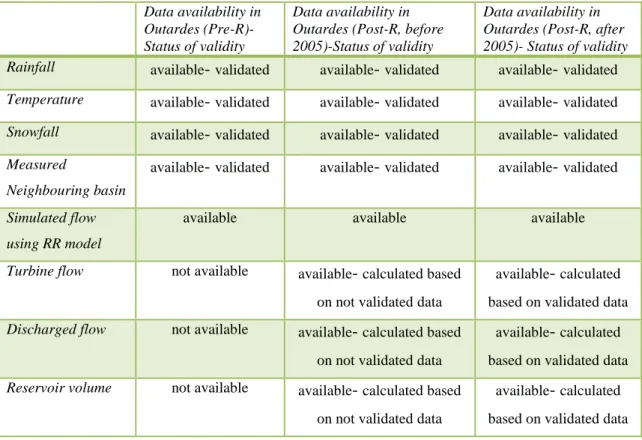
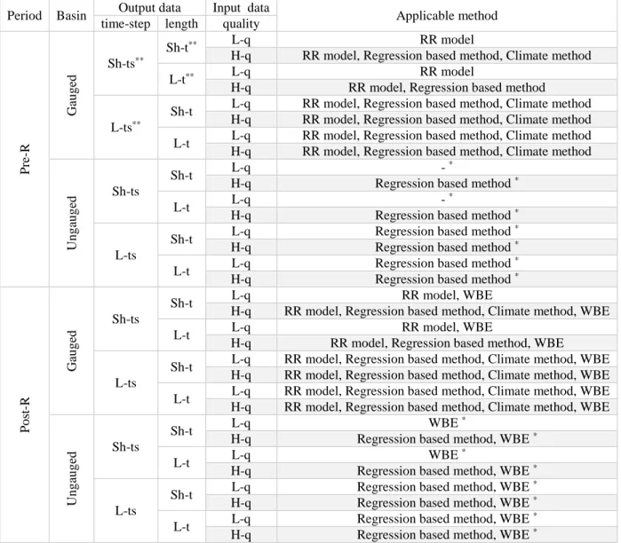
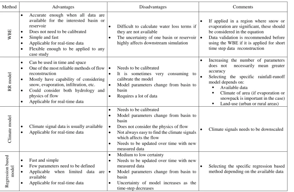
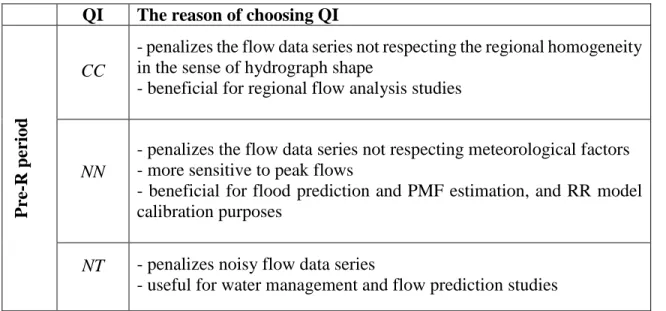
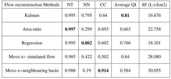
Table 3.1: Characteristics of case study basins………..40 Table 3.2: Characteristics of gauged basins in the neighbourhood of case study………..40 Table 3.3: Neighbouring basins selected for each case study in order to be used in the process of flow reconstruction (primary neighbouring basin) and reconstructed flow evaluation (secondary neighbouring basin)……….…...41 Table 3.4: List of available data and their validity situation for Outardes basin………….…...…42 Table 3.5: General characteristics of reservoirs of Outardes basin……….….……..43 Table 4.1: Preliminary algorithm for determining the applicable methods of flow reconstruction for each case………..….…..49 Table 4.2: Advantages and disadvantages of different groups of flow reconstruction methods....50 Table 4.3: Quality index comparison of WBE and area ratio………...……...55 Table 5.1: The list of applied methods for flow reconstruction during the Pre-R period…….….62 Table 5.2: The list of selected quality indexes for Pre-R period………69 Table 5.3: Comparison of QIs for a few methods of flow reconstruction (Outardes 4)………….76 Table 5.4: Comparison of QIs for a few methods of flow reconstruction during Pre-R period (Outardes 3)……….…...77 Table 5.5: Comparison of QIs for a few methods of flow reconstruction during Pre-R period (Outardes 2)………....77 Table 6.1: List of applied methods to define the parameters of suggested method for flow reconstruction during the Post-R construction period………..…..90 Table 6.2: The list of designed quality indexes for post-reservoir construction periodTable 6.3: Characteristics of studied basins for input data uncertainty……….…..99 Table 7.1: Different QIs for three methods of flow reconstruction for Post-R in Outardes 4, Outardes 3, and Outardes 2 (part 1)………..129

Table 7.1: Different QIs for three methods of flow reconstruction for Post-R in Outardes 4, Outardes 3, and Outardes 2 (part 2)……….…….130 Table 7.1: Different QIs for three methods of flow reconstruction for Post-R in Outardes 4, Outardes 3, and Outardes 2 (part 3)………..131 Table 7.1: Different QIs for three methods of flow reconstruction for Post-R in Outardes 4, Outardes 3, and Outardes 2 (part 4)………..132 Table 7.2: The average values of different terms of each 17 hydraulic system and their instrument uncertainties- q sp= Discharged flow, q tr= Turbine flow, q out = Outflow from the reservoir, q out= Inflow to the reservoir (report C1, Haché et al. 1996)………..…….…..145 Table 7.3: The average range of estimated random uncertainty (m3/s) based on different scenarios in Outardes2-2000……….……….……..151

LIST OF FIGURES

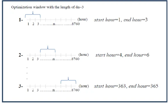
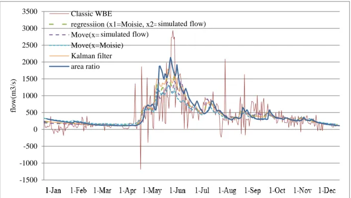
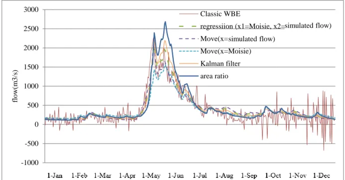
Figure i-1: Schematic of three reservoirs in series………...……….…...XXIX Figure 1-1: Schematic of thesis……….……….12 Figure 2-1: The hierarchy of developed methods for flow reconstruction and filtering in Quebec………25 Figure 2-2: The schematic of optimization window in the POM for a hypothetical year….….…29 Figure 3-1: Location of the Outardes Basin in Quebec (a and b), and sub-basins of Outardes 4, Outardes 3 (in darker color), and Outardes 2 (c), (a: https://maps.google.ca, b: www.wikipedia.org)...37 Figure 3-2: Schematic of three reservoirs of Outardes 4, Outardes 3, and Outardes 2…………..38 Figure 4-1: Schematic of methodology-Selecting the family of flow reconstructing………46 Figure 4-2: Comparison of reconstructed flow using WBE and area ratio………56 Figure 5-1: Schematic of methodology- Developing the specific flow reconstructing method and evaluating the quality and uncertainty of reconstructed flow for Pre-R period……….……59 Figure 5-2: Comparison of different methods of flow reconstruction for Outardes 4 (1966)…....71 Figure 5-3: Comparison of different methods of flow reconstruction for Outardes 4 (1968) …...71 Figure 5-4: Comparison of different methods of flow reconstruction for Outardes 4 (1970) …...72 Figure 5-5: Comparison of different methods of flow reconstruction for Outardes 4 (1971) …...72 Figure 5-6: Comparison of different methods of flow reconstruction for Outardes 4 (1981) …...73 Figure 6-1: Schematic of methodology- Developing the specific flow reconstructing method and evaluating the quality and uncertainty of reconstructed flow for Post-R period………82 Figure 6-2: The schematic of optimization window in the improved POM for a hypothetical year……….85 Figure 6-3: Schematic of the proposed Deterministic based optimization model………..93 Figure 6-4: Schematic of the Stochastic based optimization model………...96

Figure 6-5: Schematic of developed methodology for flow uncertainty analysis………..….….104 Figure 6-6: Schematic of reservoirs for which uncertainty analysis of input data is done by Hydro-Quebec………..106 Figure 7-1: Results of applying classic WBE to Outardes 3 (2009)……….….……..112 Figure 7-2: Results of applying optimization model to Outardes 3 (2009) when c=p=q=𝛾=1, dn=3……….….113 Figure 7-3: Calculated flow data series based on scenarios ai, aii, bi, and bii in comparison with optimization model, when all the parameters are set to one and dn=3, which is shown in darker color in the graphs (Outardes 3-2009)………..115 Figure 7-4: Calculated flow data series based on scenario c for two different gamma values in comparison with optimization model, when all the parameters are set to one and dn=3, which is shown in darkest color in the graph (Outardes 3-2009)………..….116 Figure 7-5: Comparison of daily flow (m3/s) calculated by classic WBE (bold line) with deterministic based optimization model solved based on different d coefficient (rest of the lines)- (Outardes 4-2008)………..……….……….119 Figure 7-6: Comparison of deterministic based model, stochastic based model, and classic WBE (Outardes 4-2005).………..……….……….119 Figure 7-7: Comparison of deterministic based model, stochastic based model, and classic WBE (Outardes 4-2009)….………..……….….120 Figure 7-8: Comparison of deterministic based model, stochastic based model, and classic WBE (Outardes 4-2011)………..……….………..120 Figure 7-9: Comparison of deterministic based model, stochastic based model, and classic WBE (Outardes 3-1995) ………..…….……….121 Figure 7-10: Comparison of deterministic based model, stochastic based model, and classic WBE (Outardes 3-1996) ………..…….……….121 Figure 7-11: Comparison of deterministic based model, stochastic based model, and classic WBE (Outardes 3-2005) ………..…….……….122

Figure 7-12: Comparison of deterministic based model, stochastic based model, and classic WBE (Outardes 3-2009) ………..…….……….122 Figure 7-13: Comparison of deterministic based model, stochastic based model, and classic WBE (Outardes 3-2011) ………..…….……….123 Figure 7-14: Comparison of deterministic based model, stochastic based model, and classic WBE (Outardes 2-1990) ………..…….……….123 Figure 7-15: Comparison of deterministic based model, stochastic based model, and classic WBE (Outardes 2-1991) ………..…….……….124 Figure 7-16: Comparison of deterministic based model, stochastic based model, and classic WBE (Outardes 2-2005) ………..…….……….124 Figure 7-17: Comparison of deterministic based model, stochastic based model, and classic WBE (Outardes 2-2009) ………..…….……….125 Figure 7-18: Comparison of deterministic based model, stochastic based model, and classic WBE (Outardes 2-2011) ………..…….……….125 Figure 7-19: Annual average QI for deterministic and stochastic methods (Outardes 2)………133 Figure 7-20: Annual average QI for deterministic and stochastic methods (Outardes 3)………133 Figure 7-21: Annual average QI for deterministic and stochastic methods (Outardes 4) …...…134 Figure 7-22: Average IR of NN, CC, and NT for deterministic and stochastic methods (Outardes 2)………..……….134 Figure 7-23: Average IR of NN, CC, and NT for deterministic and stochastic methods (Outardes 3)……….……….….135 Figure 7-24: Average IR of NN, CC, and NT for deterministic and stochastic methods (Outardes 4)……….……..135 Figure 7-25: Comparison of specific flow calculated using different methods of flow reconstruction……….………..136 Figure 7-26: Comparing the hydrograph of scaled reconstructed flow for Outardes 4, 3, and 2 with regional flow data series……….……….138 Figure 7-27: Normal Q-Q plot……….….139

Figure 7-28: Scale location plot………139

Figure 7-29: Residual versus fitted value plot……….………..……...140

Figure 7-30: Comparing the results of moving average with deterministic based model, Outardes2 (2000). a) winter low flows, b) spring high flows………..………....141

Figure 7-31: Comparison of Classic WBE, deterministic method, stochastic method, and combined flow (Outardes2-2000)……….….142

Figure 7-32: Selected year (2000) for uncertainty analysis in Outardes 2Instrument uncertainty………143

Figure 7-33: Instrument uncertainty for Outardes 2-2000………147

Figure 7-34: The results of uncertainty analysis for Outardes 2-2000-scenario I………149

Figure 7-35: The results of uncertainty analysis for Outardes 2-2000-scenario II ………..150

Figure 7-36: The results of uncertainty analysis for Outardes 2-2000-scenario III ………150

Figure 7-37: The results of uncertainty analysis for Outardes 2-2000-scenario IV …………....151

LIST OF SYMBOLS AND ABREVIATIONS

a parameter of multivariable regression ANFIS Adaptive Neuro-Fuzzy Interaction System ANN Artificial Neural Network

AO Arctic Oscillation AVE Absolute volume error

i

a Differences discharges of the days i+1 and i of the selected neighbouring basin

b Parameter of multivariable regression

j

Benefit

BMA Bayesian Model averaging

i

b Differences discharges of the days i+1 and i of the selected calculated flows

1

B , B₂ Errors of developed Kalman method

c _{Optimisation model’s parameter to allocate a weight to the set of variation variables} (Z and ₎

CC Consistency Coefficient

cj c coefficient of jth parameter set in the stochastic based model

cn Mother c parameter of iteration number n+1 in the stochastic based model

D Deterministic method

𝐷_𝑛,𝑜 Difference between the original and the new flow (𝑛𝑓_𝑑)

dn Parameter of POM which is related to number of days for which the optimization is being solved

dnj Parameter of dn for jth parameter set in the stochastic based model

dnn Mother dn parameter of iteration number n+1 in the stochastic based model

e Constant value of multiple regression method E Evaporation from the reservoir during the time Δt

inf

E Inferior squared WBE’s error

data input

E Uncertainty of flow data caused by random uncertainty of input data

sup

E

f Probability of flow

FQ Fitted line to values of LN3 of a 2-year return period GA Genetic algorithm

GLUE Generalized likelihood uncertainty estimator

int Interaction between stored water in the reservoir and groundwater

IR Improvement ratio

KPSS Kwiatkowski-Phillip-Schmidt-Shin test m Rank of the value

MCMC Markov chain Monte Carlo Move Maintenance of variance

n Number of days that the trend of both calculated flow and neighbouring basin flow is increasing or decreasing

N Total number of days

NASH Nash–Sutcliffe efficiency coefficient NAVE Normalized absolute volume error nl Length of the short record

nl + n2 Length of the long measured data

i

nbf Flow of ith day in the neighbouring basin

s

nbf Scaled flow from the neighbouring basin

F Flow caused by effective rainfall

𝑓_𝑑,𝑖 Flow calculated using disturbed input data for ith day

𝑓_{𝐷,𝑘,𝑖} Flow calculated using deterministic method for kth day of segment i

Fn Flow to reservoir number n

𝑓_𝑜,𝑖 Original flow for ith day

fRR Simulated flow using RR model

𝑓_{𝑆,𝑘,𝑖} Flow calculated using stochastic method for kth day of segment i 𝐹_{𝑊𝐴,𝑘,𝑖} Weighted average flow for the kth day of ith segment of a year

NN Normalized Nash NT Normalized Tortuosity

Offset Mean value of extreme volume values (

v

v

p Parameter of POM to allocate a weight to the variable of Z P _{Precipitation over the reservoir surface}

P (ps j) Probability of jth parameter set POM Perreault Optimization Model Pre-R Pre-Reservoir Construction Period

PS Parameter Set

Post-R Post-Reservoir Construction Period

q Parameter of POM to allocate a weight to the variable of 

cali

q

f

q Average filtered flow when i=1,…,N

fi

q

QI Quality Index

𝑄𝐼𝑎𝑣𝑒 𝑆,𝑖 Average QI of stochastic method for segment i 𝑄𝐼_{𝑎𝑣𝑒 𝐷,𝑖} Average QI of deterministic method for segment i

q

reservoir)

obs

q

Average reconstructed flow

obsi

q

q

q

discharged/spilled flow from reservoir number n)

ri

q

simn

q

q

q

WBEi

q

𝑟𝑎𝑛𝑔𝑒_𝑁𝐹 Possible range of flow data series (total uncertainty

Rl Predicted lower range

Rn Reservoir number n

RR Rainfall-Runoff

Ru Predicted upper range

S Stochastic method

s Surface of the basin

s

s

sf

SFR Specific flow ratio

sf

T Tortuosity

TM Thornth waite-Mather

(min) inf

v

v

) inf(n

v

) (n

v

(max) sup

v

_v

) sup(n

v

m3_/s)

w1, w1, w1 Weight of QIs for defining the fitness in stochastic based method

𝑤

𝑤

WBE Water balance equation WSS Wide Sense Stationary xi Measured data for day i

Y Reconstrcuted flow using the Kalman filter based model y1 Filtered simulated flow using the Kalman filter method

y2 Filtered neighbouring basin’s flow using the Kalman filter method

𝑌̂ _𝑖 Reconstructed flow using Move III for the day i

Z Flow variation during 2 consecutive days

1

 ,₂ Coefficients of developed Kalman method



j





n





 Flow variation during 3 consecutive days

∆_{𝑖𝑛𝑝𝑢𝑡 𝑑𝑎𝑡𝑎} Uncertainty of flow caused by instrument uncertainty ∆𝑞𝑖𝑛 Instrument uncertainty of qin

∆_{𝑞𝑜𝑢𝑡} Instrument uncertainty of qout

∆𝑣𝑜𝑙𝑢𝑚𝑒 Instrument uncertainty of volume ∆𝑥_𝑖 Absolute uncertainty of measured 𝑥_𝑖

Δsn Storage volume changes in the reservoir number n

𝜇̂ _𝑦 Unbiased estimator of the mean of the complete extended record in Move III 𝜎̂_𝑦 Unbiased estimator of the variance of the complete extended record in Move III

LIST OF APPENDICES

ARTICLE 1: An Algorithm for Selecting The Most Appropriate Method of Natural Flow Reconstruction in Hydropower Reservoirs...170 ARTICLE 2: Natural Flow Reconstructing in Ungauged Basins Using New Kalman Filter and Water Balance Based Methods (Part 1: Theory)…….………..……….…..197 ARTICLE 3: Natural Flow Reconstructing in Ungauged Basins Using New Kalman Filter and Water Balance Based Methods (Part 2: Case Studies, Results and Discussion)...223

GLOSSARY

Flow:

Flow is defined as the runoff caused by effective rainfall. Flow can be calculated using the classic Water Balance Equation (WBE) for a reservoir (as a closed system):

Fn=qout,n - qin,n+ (ΔSn/Δt) (i-1)

where:

qout,n…..= the summation of outflow from the reservoir number n (Rn) during the

sampling time period,

qin,n = the summation of inflow to reservoir number n during the sampling time

period,

ΔSn = the net change of storage volume in the reservoir number n during the

sampling time period, Δt = the sampling time period

Fn = the unknown flow value caused by effective rainfall (which includes all the

minor terms such as evaporation, direct rainfall, and interaction between surface water and ground water) to reservoir number n.

As illustrated in Figure i-1, qin,n is equal to the regulated outflow from the upstream reservoir (if

available), qout,n-1, which is the summation of turbine flow from the reservoir number n-1 (qtr,n 1)

Figure i-1: Schematic of three reservoirs in series

Ungauged basin:

An ungauged basin (with or without a reservoir) is defined as a basin that does not have available or recorded river flow measurements or data.

Uncertainty:

“The component of a reported value that characterizes the range of values within which the true value is asserted to lie” (NDT resource center, 2014).

(Note: In this project, the uncertainty in a flow data series could be caused from the uncertainty of the methods’ structure (WBE, optimization model, and etc.) and/or input data uncertainty)

Noise:

Noise is defined as obvious uncertainty and expressed as the spurious variation exhibited in a data series. Usually a data series’ uncertainty cannot be detected by looking at data series’ graph; however, noise is visually distinguishable when data values are plotted on a graph.

Fn+1 Rn Rn+1 Rn-1 Fn qtr,n qtr,n-1 qsp,n qsp,n-1 qout,n-1= qin,n qout,n= qin,n+1

In the work presented in this thesis, the flow data series are considered noisy, from a variation standpoint, when they clearly differ from the neighbouring basin’s flow and rainfall-runoff model’s flow.

Automatic model:

An automatic model is defined as a method which is independent from a human’s decision and uncertainty. Automatic models could act like a type of software which takes input data and produces one or more output data. Thus, the output values will not require manual modification. Like software, the parameters of the automatic model would change depending on case study scenarios.

CHAPITRE 1

INTRODUCTION

1.1

Context of Thesis

Locally and regionally reliable flow data series (pre- and post-reservoir construction period) are essential for the purpose of analyzing flow frequency, simulating hydraulic systems, predicting the flow, designing hydraulic structures, and undertaking other activities related to water planning and management. Poor flow data records, however, may exacerbate the uncertainty of water management. For example, a lack of reliable flow data values affects water allocation studies and may result in deficiencies in hydropower production, irrigating plans, etc. As well, unreliable knowledge about flow results in poor flow prediction, leading to a lack of proper preparation for possible floods or droughts, causing irreparable financial or human loss. These examples show how unreliable flow data series affect socio-economic aspects of people’s life and government’s services, directly and indirectly.

The discussion of obtaining reliable flow data holds importance for Quebec (and for any other region with the same characteristic) as this province possesses 2 percent of all of the planet’s freshwater, with potential use for many purposes such as agriculture, tourism, hydropower, and industry. As an example, in 2006, the province of Quebec produced 205.661 TWh of hydroelectricity, while “the clear exports of electricity have been established at 6,3 TWh for the same year” (ROBVQ, 2013). In 2004, Canada was the fourth largest producer of hydroelectricity in the world, with Quebec producing almost 50% of the total hydroelectricity in Canada (ROBVQ, 2013). Systematic management and usage of Quebec’s water resources are feasible only if reliable data (including flow) is available. Flow is not measured in many of the basins of Quebec (neither the period when basins did not possess a reservoir nor the time period when they are equipped with reservoirs) because of the vastitude of province and inaccessibility of many of the catchments. Therefore flow needs to be estimated with reasonable accuracy.

A project was initiated by Hydro-Quebec entitled “reconstructing the flow data for ungauged basins of Quebec” in order to estimate the flow values of ungauged basins in Quebec. The project addressed the flow estimating methods for the Quebec’s basins where the flow is not measured. It was necessary for Hydro-Quebec to conduct this project because of the claim that more reliable

flow data increases the justification of water resource management and in turn will help the production of hydroelectricity by a considerable amount.

The main topic of this PhD thesis is to study the methods of reconstructing and obtaining reliable flow data when they are not readily available. This research was conducted within the framework of the Hydro-Quebec’s “Reconstructing the flow data for ungauged basins of Quebec” project. The nature of the Hydro-Quebec’s project has always encountered shortfalls in the existing studies and the intention of this work is to address and resolve these inadequacies. Some of the shortfalls encountered are listed below:

A)

:

There exist many different methods of flow reconstruction. Selecting the appropriate method in each time period depends on different factors. For instance, the following six factors should be considered when selecting a method for basins within the province of Quebec:

1. Flexibility of method

The data reconstruction method needs to be flexible enough to be applicable for all the basins in Quebec, as most of them are ungauged.

2. Scale of reconstructed flow

The main reasons for reconstructing flow data values are to improve the processes of water resource management, flow prediction, and risk management. These goals are achievable with long-term (historical and real-time1) daily flow data; therefore, flow reconstruction is required to be done on a daily and long-term basis.

1 _{Real-time data are the data related to the present time step. For example, the real-time daily flow is the flow of the}

3. Quality of reconstructed flow

As flow data are used for short term flow prediction and management, high-quality flow data is required because it may be difficult to efficiently analyze flow series affected by noise disturbing the short/long term memory of flow data (as flow analysis methods are based on the memory and behaviour of data series in time). Flow noise results in uncertainty of sometimes millions of cubic meter of estimated flow volume each day 2.

Also, high quality reconstructed flow data result in more efficient water resource planning and management in long term.

(Note: both snowmelt and evaporation are factors that can affect flow data, especially in large basins and reservoirs. Thus, accounting for these factors may improve the flow reconstruction results)

4. Applicability of method

One important objective of flow reconstruction is to predict future flow values (usually a few days in advance), which is usually possible by knowing the real-time flow data (predicting flow data is out of the scope of this study). Thus, any method employed should be applicable to both historical and real-time data.

5. Data availability

The flow reconstruction method should be selected based on available data. As most watersheds in Quebec are ungauged, the measured data obtained are limited to:

- Pre-Reservoir (Pre-R) Period: the flow data series measured in neighbouring basins to that of the studied basin (few neighbouring basins), and hydrologic data (including daily rainfall, daily minimum temperature, daily maximum temperature, daily temperature, and daily snowfall) of the studied basin.

- Post-Reservoir (Post-R) Period: the flow data series measured in neighbouring basins to that of the studied basin, hydrologic data (including daily rainfall, daily minimum

2 _{For example, 15 m}3_{/s of flow noise is equal to (15*24*3600 = 129600) 129600 m}3 _{of uncertainty in volume of flow}

temperature, daily maximum temperature, daily temperature, and daily snowfall) of the studied basin, as well as reservoir related data of the studied basin such as water level on the upstream and downstream side of the reservoir, gate openings, and produced electricity. These reservoir data have been used by Hydro-Quebec to calculate turbine flow, discharged flow and reservoir volume.

Thus, the flow reconstruction method may be different for Pre-R and Post-R time periods. Also, it is preferable to include as much data as possible in the flow reconstruction process because they empower the flow estimation values by taking into account different aspects of this topic.

(Note: Hydro-Quebec already used hydrologic data to simulate flow using a Rainfall-Runoff (RR) model. The results of this simulation are available for both Pre-R and Post-R periods.)

6. Quality of input data

7. It is known that the quality of input data affects the results of the flow reconstructing method. Therefore, available hydrologic data and neighbouring basin’s flow data must be of high quality and reliability. On the other hand, reservoir related data (including turbine flow, discharged flow, and reservoir volume) prior to 20053 _{(considered as raw data) may} contain uncertainties and noises during certain time periods.

The fundamental topic of developing a flow reconstruction and validation method for ungauged basins in Quebec that considers these six factors has always been a constant debate. However, there is no research results available on how to select the appropriate

3 _{For the years after 2005, the water level on the upstream and downstream side of the reservoir, produced electricity,}

and system’s characteristics are validated, and thus, the calculated discharged flow, turbine flow, and storage volume data for post-2005 are more reliable. However, before 2005, discharged flow, turbine flow, and storage volume data taken from Hydro-Quebec data base are calculated based on non-validated measured data. It means that these data are raw and they may contain noise and/or outlier.

method of flow reconstruction that puts into consideration the different aforementioned factors that affect choice of method for the province of Quebec (Question # 1).

B) Lack of a flexible methodology in reconstructing reliable daily flow data series:

During the past few decades, a lot of effort has been devoted to reconstructing plausible flow data series that can be used to validate flow data, and to estimate the uncertainty of hydraulic systems in Quebec (i.e. Perreault et al. 1996, Bennis et al. 1994, Bennis and Kang, 2000, and Haché et al. 2003). Some of these studies are listed below:

- Bisson and Roberge (1985) developed a rainfall-runoff (RR) model to simulate flow in the basins of Quebec; however, this model usually underestimates peak flows.

- Charbonneau and Berube (1987) and Berrada et al. (1996) proposed separate methods to remove noise from flow data series (filter flow data series) that were calculated using WBE; but ultimately, because these methods required knowledge of future data, they could not be used in real-time situations.

- Perreault et al. (1995) suggested a procedure to improve flow data series by combining the results from rainfall-runoff (RR) model, WBE, and neighbouring basin’s filtered flow (reconstructed flow using their suggested method which has been applied in a nearby basin). However, this method may overestimate the cumulative amount of flow for a period of certain number of days (Nguyen and Bisson, 1998).

- Nguyen and Bisson (1998) suggested a regression and exponential smoothing technique to solve the problems of the Perreault’s model (1995). In their method the validated flow for each day is regarded as an exponential function of previous days’ flow. This method is acceptable when data are stationary; in reality, a more appropriate method is required to take into account seasonality effects on flow. Moreover, it would be preferable to calculate a more accurate flow data series by filtering the Water Balance equation (WBE) series using all available flow data of basin (such as flow from RR model and neighbouring basin, etc.).

- Lastly, Hydro-Quebec currently uses a method that adopts a mostly manual procedure for calculating and filtering flow data values. In this method, flow values are calculated

using WBE and then modified by taking into consideration regional and temporal analysis. However, the results obtained using this method may be affected by human-caused uncertainties and misjudgments, requiring a method that eliminates human error. - Thus, Perreault (2011) suggested a WBE based optimization model (POM) which is independent from human judgment. This model reconstructs and filters hourly flow data series and attempts to minimize the variation of flow data and WBE errors (this model is described in more details in Chapter 2). Despite the fact that POM is successful in reducing noise and removing unrealistic values, it still has some deficiencies and problems. For example:

(1) this method is dependent on volume data of 5-minute intervals (not applicable when data of 5-minute intervals are not available),

(2) it is only applicable for an hourly time scale,

(3) the parameters of this model are constant during the time and space,

(4) this model does not take into account available data from rainfall-runoff model and neighbouring basins to improve results,

(5) results are still susceptible to noise, especially for low flows.

All of the studies mentioned above were important steps towards enhancing the knowledge of flow data series in the province of Quebec. Nevertheless, all of the methodologies developed for ungauged basins in Quebec (except for the developed RR model by Bisson and Roberge, 1985) were based on WBE, and thus, only applicable for Post-R period when the input data of WBE (turbine flow, discharged flow, and reservoir volume) are available. However, reconstructing daily flow data values for Pre-R period has remained almost unexplored. Knowing the values of flow for Pre-R period is helpful in that it provides a more comprehensive understanding of historical flow data, which helps to perform more reliable flow analysis. Accordingly, the second question is how to reconstruct daily flow for Pre-R period (Question # 2).

Even for the Post-R period, none of the research mentioned above provide a flexible methodology to reconstruct and validate reliable daily flow data series that is independent

of human decisions. This gives rise to an interesting question of how toreconstruct more likely values for daily flow for Post-R period (Question # 3).

C) Lack of criteria to evaluate the quality of the reconstructed flow in ungauged basins: An important topic related to the flow reconstruction studies is how to assess the performance of flow reconstruction methods. Usually, researchers would apply one or two quality indexes (QIs) to evaluate reconstructed data series (e.g. Mean Square Error by Gupta et al. (2009), temporal or spatial correlation coefficient, and Nash-Sutcliffe Efficiency by Johnston et al. (2009)). These methods adopt different techniques when comparing the reconstructed data with a measured data series. However, the topic is more challenging when there is no measured data series that can be used as reference data (same as current study). In the research mentioned above which applies to Quebec, traditional QIs were used in the comparison of reconstructed flow data with existing filtered flow series (the mostly manually filtered flow series are available in Hydro-Quebec’s database). As the filtered flow values are less reliable prior to 2005 (as the input data may contain uncertainties before 2005), it will be advantageous to design a few different QIs to evaluate the quality of the reconstructed flow values that are independent from filtered flow values. This challenge raises the questions of how to evaluate the quality of the reconstructed flow data series for ungauged basins (Question # 4).

D) Lack of a methodology to analyze the uncertainty of reconstructed flow in ungauged basins: Another indispensable element related to hydrological studies (aside from flow data reconstruction) is uncertainty analysis. There are many different methods available to evaluate different types of uncertainty. For instance, Generalized Likelihood Uncertainty Estimator (GLUE), Markov Chain Monte Carlo (MCMC), and most existing sensitivity analysis methods are used to define the parameter of uncertainty. The Bayesian model is also another method which factors in uncertainty in input data, output parameters, and the model’s structure (Yang et al. 2007). Most of the existing methods are dependent on the measured data. Therefore, it is still a challenge to find out how to evaluate the uncertainty of flow data in ungauged basins (Question # 5).

As the previous researches could not find answers to the above mentioned questions (Questions # 1-5), the goal of this study was to find solutions to these questions. In fact, the mentioned questions formed the base of the objectives of this thesis.

1.2

Motivation

The driving force in finding solutions to the questions mentioned above (as explained in section 1.1) were because of the importance of this topic, coupled by a lack of the following tools for our research:

 an algorithm to select the most appropriate family of flow reconstruction method considering different factors,

 a flexible methodology to reconstruct daily flow data series for Pre-R period,

 an automatic flexible method (independent from a human’s decision and uncertainty) for Post-R period,

 the indexes to evaluate the quality of reconstructed flow in ungauged basins, and  a methodology to analyze the uncertainty of reconstructed flow in ungauged basins. The desire to find solutions to the above questions also enhanced the desire of taking the next step towards reaching the final goal; the ability to estimate more reliable flow data series for ungauged basins of Quebec.

1.3

Objectives

The general objective of this research is to develop a method to obtain daily flow values for ungauged basins in Quebec for both Pre-R and Post-R periods. To attain this primary objective, five secondary objectives had to be completed in the course of this research. These include (Figure 1-1):

a) Introducing an algorithm for selecting the most appropriate family of flow reconstruction methods in each case study (Pre-R and Post-R periods).

The motivation for this came from the fact that currently there is no completely recognized methodology available to help researchers in selecting an appropriate method of flow reconstruction. This objective aims to find the answer to Question # 1 mentioned in Section 1.1. The developed algorithm based on this objective should consider all the 6 factors mentioned in Section 1.1 that affect the selection of flow reconstruction method in the area. According to the suggested algorithm, WBE based methods and regression based methods are the most appropriate family of flow reconstruction methods in the current case-study for Post-R and Pre-R periods, respectively.

b) Evaluating the performance of existing methods of flow reconstruction, and defining the weaknesses in them.

Before developing a methodology for flow reconstruction, it is necessary to assess the capabilities and weaknesses of the existing flow reconstruction methods that are currently being used.

c) Developing an optimization method based on Kalman filter4 as a tool to combine the available data and produce flow values for Pre-R, and an automatic WBE based model to reconstruct daily flow for Post-R periods.

This objective was formed to develop a flexible regression based methodology for the Pre-R period, and an adjustable automatic WBE based model for Post-Pre-R period. This objective addresses Questions # 2 and # 3 mentioned in Section 1.1.

d) Designing criteria applicable to ungauged basins in order to evaluate the performance of developed methods.

After reconstructing the flow data series, an assessment of the data quality is required. This objective was designed to address Question # 4, mentioned in Section 1.1.

e) Evaluating the uncertainty of the reconstructed flow in ungauged basins.

It is always helpful to define the confidence level of estimated data series. This objective was designed to analyze the uncertainty of flow data series and respond to Question # 5, mentioned in Section 1.1.

1.4

Content of Thesis

The content of this thesis is summarized in Figure 1-1:

- Chapter 1 provides an introduction to the subject, problem, motivation, and the objectives. - Chapter 2 gives a literature review of the different methods and models of flow reconstruction

for Pre-R and Post-R periods, existing methods of quality evaluation, and techniques of uncertainty analysis.

- Chapter 3 explains the case study presented in this thesis. This chapter discusses the available data and information for the area, as well as the quality of this data. In this research, the methodology and the result are divided into a few sub-methodologies and sub-results related to Pre-R and Post-R periods because the results of each sub-methodology define the approach of next step. The sub-methodologies and sub-results are presented in Chapters 4, 5, 6 and 7. Therefore, the case study is presented before them in Chapter 3.

- Chapter 4 introduces an algorithm that helps to select the most appropriate family of flow reconstruction method to different scenarios, with consideration to the applicability, advantages and disadvantages of reviewed methods in Chapter 2. This algorithm factors in all determinative parameters that can affect the selection of appropriate methods of flow reconstruction. It is then applied and tested in our case study. This algorithm and the results of its application to the case study are presented in this chapter to fulfill Objective a, and provide answer to Question # 1, stated in Section 1.1. The content of this chapter has been submitted to Canadian Water Resource Association (CWRA) in 2013 in the form of a journal paper. The submitted version of this papers is presented in appendix 1.

- Chapter 5 suggests a methodology for reconstructing daily flow for the Pre-R period (satisfying

the results are then compared to those of a few existing methods. The comparison is done using visual graphs with a few suggested QIs.

- In Chapter 6, several existing methods of flow reconstruction (classic WBE and POM) for Post-R period will be first assessed (Objective b). Then, an optimization model will be developed based on POM. Lastly, a sensitivity analysis will be done on the optimization method to evaluate the authenticity of its assumptions and the necessity of improving them. Then, the developed methodology for automatizing the suggested optimization model for Post-R period will be explained (achieving Objective c and answering Question # 3). A few QIs that are applicable to ungauged basins are then introduced to evaluate the reliability of reconstructed flow values and compare the results with classic WBE. A methodology will also be presented to evaluate the regional and temporal homogeneity of the flow data series (Objective d). A methodology for analysing the uncertainty and defining the range of reconstructed flow is presented in this chapter to fulfil Objective e.

Chapter 7 will present the results of applying all the presented methodologies in Chapter 6 to a case study.

Chapters 5, 6, and 7 will provide answers to Questions # 4 and 5 mentioned in Section 1.2. The content of these chapters has been published in the form of two journal papers at Journal of Hydrologic Engineering (ASCE). The accepted version of these papers are presented in appendices 2 and 3.

Finally, conclusion and recommendations are presented at the end of the thesis. The limitations of developed methodology in this thesis are also listed in this section.

Figure 1-1: Schematic of thesis

Objective e:

Evaluating the uncertainty of NF.

Objective d:

Evaluating the performance of developed methods.

Objective c:

Developing a methodology to reconstruct the daily flow.

Objective b:

Evaluating the performance of existing methods of flow reconstruction

Objective a:

Proposing an algorithm for selecting the most appropriate family of flow reconstruction method in each case study (Pre-R and Post-R periods)

Methodology

Chapters 2, 4: - Literature review.

- Developing the algorithm based on literature review

Chapter 6:

- Comparing the results of classic WBE to POM.

- Doing a sensitivity analysis on POM. Objectives

Chapters 5, 6:

- Developing a Kalman filter based method for Pre-R period

- Developing a an automatic optimization model for Post-R period

Conclusion and recommendations

Chapters 5, 6: - Designing few QIs

- Evaluating the regional and temporal homogeneity of reconstructed flow data

Chapter 6:

-Applying a sensitivity

analysis method to evaluate

the uncertainty of

reconstructed flow.

Chapter 7 Chapters 5, 7 Chapters 5, 7 Chapter 7

Results and conclusion

CHAPITRE 2

LITERATURE REVIEW

2.1

Introduction

In this chapter, a general literature review is presented on different flow reconstruction methods available for Pre-R and Post-R period. This is followed by a summarized explanation of the existing methods for data series evaluation including QIs, recent methods used to assess stationarity and regional homogeneity of flow data series. A literature review is also presented on the available methods used to analyse the uncertainty found in flow data series.

2.2

Flow Reconstruction

In the past several years, many different methods and models have been developed to simulate or extend flow data in gauged or ungauged basins. In this chapter, these methods are grouped in three main categories based on their approach to simulate flow:

 hydrologic methods,  hydraulic methods,

 and regression-based methods.

The applicable flow reconstruction methods may be different for Pre-R and Post-R period because the available data, information, and the basins’ condition, are usually different for these two time periods. The categories of flow reconstruction methods (hydrologic, hydraulic, and regression-based methods) which can be applied for each Pre-R and Post-R period are explained in the following section.

2.2.1 Pre-R Period

In the case of basins without a reservoir (Pre-R period), hydrologic data, climate data, and/or catchment characteristics can be measured. Thus, hydrologic or regression based methods, which depends on these types of data, may be used for flow reconstruction.

2.2.1.1 Regression based methods

Regression-based methods are those developed based on a mathematical relationship between the flow of the study basin (as a dependent variable) and independent variables from the same or the neighbouring basins. These methods are simple and fast to use (Rezaeianzadeh et al. 2013). An example of a regression-based methods is one that estimates the flow data of the interested sub-basin using available flow data of the main sub-basin. For example, there exists one method that calculates the stream flow of an ungauged sub-basin by relating the ratio of the slope and area of that sub-basin to those of the main basin (Schreiber and Demuth, 2002).

When flow data of neighbouring basins are available, a logarithmic relation (logarithmic scaled data helps to obtain residuals that are approximately symmetrically distributed around zero) can be developed between the flow data characteristics of the neighbouring basins and applied to the basin of interest (using regression method in space). For example, Jones et al. (2004) applied a regression-based method to relate the logarithmic values of measured river-flow to linear combinations of soil moisture and effective precipitation. They then applied this regression equation to the ungauged basin of interest to calculate the flow data series. Also, Wen (2009) tried to reconstruct flow by relating the discharge time series to rainfall and maximum temperature. Hughes and Smakhtin (1996) explained that a potential method of extending the flow of a basin of interest would be to simply weight the observed streamflow values of one or more neighbouring gauged basins by the ratio of the catchment area of the basin of interest to the area of the gauged neighbouring basins. The problem with this method is that the flow values of adjacent basins are rarely linearly related to the catchment area of the basin of interest as they may have different hydrology and morphology. Also, it is possible to have a trend of non-stationarity in the actual stream flow data series at the sites or stations used for interpolation (Hughes and Smakhtin, 1996). Thus, it is not recommended that flow values of neighbouring basins be directly transferred to the flow characteristic of a basin of interest.

A regression method can also be developed based on the available short-term data of a basin and used to extend the flow series over a whole time interval (regression method in time) of that basin. Simple regression between a basin’s short-term flow data series and the long-term flow data series of a nearby basin (Hernandez-Henriquez et al., 2010, Dastorani et al. 2010) exemplifies this type of regression based method. In a case study by Taylor et al. (2006), they developed a

statistically-linear model based on regression of rainfall and short-term runoff data. Since the complete rainfall data were available for their case study, a regression based method was applied to extend flow data over the whole period.

Maintenance of variance (Move) is another regression-based method for data reconstruction that preserves both mean and variance, and therefore works better than the linear-regression method (Koutsoyiannis and Efstratiadis, 2007). The Move technique reconstructs flow based on a linear regression (𝑦̂ = 𝑎 + 𝑏𝑥_{𝑖 𝑖}) in which the variables a and b were calculated in a special way (Moog et al. 1999). For example, Move.I and Move.II (Hirsch, 1982) reproduce the same first and second moments when they generate the entire sequences of 𝑦̂, where i=1,...,n𝑖 1+n2 (n1 is the length of the

short record and n1+n2 is the length of the long record), compared to historical samples. However,

in practice, Move is used to generate 𝑦̂ with i= n_𝑖 1+1,...,n1+n2 (Vogel and Stedinger, 1985). Thus,

Move.I and Move.II did not achieve its intended objective. This problem was resolved with the development of Move.III (Matalas and Jacobs 1964).

In general, regression based methods have few independent variables and usually do not take the physical characteristics or dynamics of a system into account. This reduces data authenticity, especially when they are used to reconstruct or extend short time-step and long-term flow values. Thus, it is more reliable to apply the hydrologic models that use both the hydrological and the physical data (such as characteristics of the catchment) for reconstructing flow data values.

2.2.1.2 Hydrologic methods

Hydrologic models use hydrologic data or climate data5 _{(Hwang et al. 2005) to calculate the flow.} Different studies have been undertaken to develop a relationship between the flow and climate signals in order to identify the predictability of flow or possibility of a non-random pattern in space or time (Fortin, 2001) and in most cases, a significant statistical link has been observed (Fortin and Slivitzky, 2000). Fortin (2001) found that climate has an obvious influence on runoff; he evaluated

5 _{In this thesis, ‘hydrologic data’ is referred to data such as precipitation, temperature, evaporation, and etc., but}

the reliability of different climatic indices to see if there was a non-random pattern in space or time, and identified a statistically significant link between Arctic Oscillation (AO) and runoff in northern Quebec. However, the correlation was found at times to be caused by extreme climate conditions. According to Fortin and Slivitzky (2000), river flow often correlate well with the winter temperatures, suggesting that winter temperature could be an indicator of how the regional climate is affected by the global phenomenon of AO. But while the performance of climate-based flow reconstruction methods is good in some areas, some questions remain as to their level of confidence.

RR models are the main group of hydrologic models that are most often used to estimate runoff in time and space. They can estimate runoff at different time-steps in different hydraulic systems and land uses, given that limited measured flow data is available in order to calibrate the model. RR models can range from a simple relation between rainfall and runoff to complex models that also consider the hydrologic and physical characteristics of a region.

Examples of RR models are Thornthwaite-Mather (TM) for calculating monthly flow (e.g. Taylor et al. 2006), StormNET for calculating daily or even smaller timescale flow (e.g. Karamouz et al. 2011), and the Wright model to calculate mean monthly or daily flow (Adeloye and Nawaz, 1998). Hydrotel is another RR model developed in the mid-1980s in Quebec and has been used extensively in this province for its ability to factor in the area’s meteorological condition by considering snow packs and snow melt. Hydrotel is a physically-based distributed hydrological model that can be run for hourly to daily time steps. In this model, spatial variations in watershed characteristics are taken into account using GIS and remote sensing data (Fortin et al. 2006). However, when only meso-scale grid data are available, high resolution data should be calculated from standard meteorological station data using a disaggregation model. In addition to downscaling, calibration is another inconvenience of Hydrolet because it is very time consuming.

HSAMI is another RR model developed by Bisson and Roberge (1985) to simulate the hourly or daily flow series values in Quebec’s watersheds. HSAMI is a linear reservoir-based lumped conceptual hydrological model which uses a watershed as a transfer function, whereas the meteorological conditions are used as input data, and has as its output the flow values at the outlet of the catchment. The parameters of this model include five data categories: evaporation, vertical flow (such as rainfall), horizontal flow (such as upstream flow), surface runoff and snow. It has