Branching Brownian motion with selection

(1)

HAL Id: tel-00741368

https://tel.archives-ouvertes.fr/tel-00741368

Submitted on 12 Oct 2012

HAL is a multi-disciplinary open access archive for the deposit and dissemination of sci-entific research documents, whether they are pub-lished or not. The documents may come from teaching and research institutions in France or abroad, or from public or private research centers.

L’archive ouverte pluridisciplinaire HAL, est destinée au dépôt et à la diffusion de documents scientifiques de niveau recherche, publiés ou non, émanant des établissements d’enseignement et de recherche français ou étrangers, des laboratoires publics ou privés.

Pascal Maillard

To cite this version:

Pascal Maillard. Branching Brownian motion with selection. Probability [math.PR]. Université Pierre et Marie Curie - Paris VI, 2012. English. �tel-00741368�

(2)

Probabilités et

Modèles Aléatoires et Marie Curie

École Doctorale Paris Centre

Thèse de doctorat

Discipline : Mathématiques

présentée par

Pascal Maillard

Mouvement brownien branchant avec sélection

(Branching Brownian motion with selection)

dirigée par Zhan Shi

Rapporteurs :

M. Andreas Kyprianou University of Bath

M. Ofer Zeitouni

University of Minnesota

& Weizmann Institute of Science

Soutenue le 11 octobre 2012 devant le jury composé de :

M

me

_{Brigitte Chauvin}

Université de Versailles

examinatrice

M. Francis Comets

Université Paris 7

examinateur

M. Bernard Derrida

Université Paris 6 et ENS examinateur

M. Yueyun Hu

Université Paris 13

examinateur

M. Andreas Kyprianou University of Bath

rapporteur

(3)

Université Pierre et Marie Curie 4, place Jussieu 75 005 Paris Case courrier 188 4, place Jussieu 75 252 Paris cedex 05

(4)

À Pauline, le soleil qui la fait vivre et lui est source de joie et de bonheur

(5)

(6)

Remerciements

Je tiens à remercier chaleureusement mes deux rapporteurs Andreas Kyprianou et Ofer Zeitouni ainsi que les examinateurs Brigitte Chauvin, Francis Comets, Bernard Derrida et Yueyun Hu. J’admire les travaux de chacun et c’est un grand honneur qu’ils aient accepté d’évaluer mon travail.

Merci à mon directeur Zhan Shi qui m’a fait découvrir un sujet aussi riche et passionnant que le mouvement brownien branchant, qui m’a toujours soutenu et prodigué ses conseils, tout en m’accordant une grande liberté dans mes recherches. Je remercie également les autres professeurs de l’année 2008/2009 du Master 2 Processus Stochastiques à l’UPMC pour la formation exceptionnelle en probabilités sans laquelle cette thèse n’aurait pas été possible.

Certaines autres personnes ont eu une influence directe sur mes recherches mathématiques. Je remercie vivement Julien Berestycki qui, par son enthousiasme infini, a su donner une impulsion nouvelle à mes recherches. Merci à Olivier Hénard, mon ami, pour avoir partagé à de nombreuses occasions sa fine compréhension des processus de branchement. Merci à Louigi Addario-Berry, Elie Aïdékon, Louis-Pierre Arguin, Jean Bérard, Nathanaël Berestycki, Jason Schweinsberg, Damien Simon, Olivier Zindy pour m’avoir soutenu, conseillé, éclairé.

Merci encore à Yacine B, Pierre B, Reda C, Leif D, Xan D, Nic F, Clément F, Patrick H, Mathieu J, Cyril L, Thomas M, Bastien M et Matthew R pour ce “aahh” de compréhension survenu après une discussion spontanée ou après des heures de travail en commun. Merci aux anciens et actuels doctorants du LPMA pour un quotidien stimulant, agréable et drôle et pour avoir supporté mes mauvaises blagues au déjeuner et mes questions idiotes au GTT (ou l’inverse). Merci également à l’équipe administrative du LPMA pour leur travail efficace et leur dévouement.

Merci, Danke, Hvala, Thank you à mes amis, mathématiciens ou non, de Paris ou d’ailleurs, que j’ai eu la chance de rencontrer sur mon chemin. Merci aux superbes femmes de Pierrepont et à JP. Danke an meine Familie aus dem Norden.

Et finalement, les plus grands remerciements vont à Gérard, Elsbeth, Tobi, Karin et André pour leur soutien inconditionnel, et surtout à Pauline, la seule personne qui sache aussi bien me faire tourner la tête qu’y mettre de l’ordre quand elle tourne en rond.

(7)

(8)

Résumé

Dans cette thèse, le mouvement brownien branchant (MBB) est un système aléatoire de particules, où celles-ci diffusent sur la droite réelle selon des mouvements browniens et branchent à taux constant en un nombre aléatoire de particules d’espérance supérieure à 1. Nous étudions deux modèles de MBB avec sélection : le MBB avec absorption à une droite espace-temps et le N -MBB, où, dès que le nombre de particules dépasse un nombre donné N , seules les N particules les plus à droite sont gardées tandis que les autres sont enlevées du système. Pour le premier modèle, nous étudions la loi du nombre de particules absorbées dans le cas où le processus s’éteint presque sûrement, en utilisant un lien entre les équations de Fisher–Kolmogorov–Petrovskii–Piskounov (FKPP) et de Briot–Bouquet. Pour le deuxième modèle, dont l’étude représente la plus grande partie de cette thèse, nous donnons des asymp-totiques précises sur la position du nuage de particules quand N est grand. Plus précisément, nous montrons qu’elle converge à l’échelle de temps log3N vers un processus de Lévy plus une dérive linéaire, tous les deux explicites, confirmant des prévisions de Brunet, Derrida, Mueller et Munier. Cette étude contribue à la compréhension de fronts du type FKPP sous l’influence de bruit. Enfin, une troisième partie montre le lien qui existe entre le MBB et des processus ponctuels stables.

Mots-clefs

Mouvement brownien branchant, sélection, équation de Fisher–Kolmogorov–Petrovskii– Piskounov (FKPP) bruitée, équation de Briot–Bouquet, mesure aléatoire stable.

Branching Brownian motion with selection

Abstract

In this thesis, branching Brownian motion (BBM) is a random particle system where the particles diffuse on the real line according to Brownian motions and branch at constant rate into a random number of particles with expectation greater than 1. We study two models of BBM with selection: BBM with absorption at a space-time line and the N -BBM, where, as soon as the number of particles exceeds a given number N , only the N right-most particles are kept, the others being removed from the system. For the first model, we study the law of the number of absorbed particles in the case where the process gets extinct almost surely, using a relation between the Fisher–Kolmogorov–Petrovskii–Piskounov (FKPP) and the Briot–Bouquet equations. For the second model, the study of which represents the biggest part of the thesis, we give a precise asymptotic on the position of the cloud of particles when N is large. More precisely, we show that it converges at the timescale log3N to a Lévy process plus a linear drift, both of them explicit, which confirms a prediction by Brunet, Derrida,

(9)

FKPP type under the influence of noise. Finally, in a third part we point at the relation between the BBM and stable point processes.

Keywords

Branching Brownian motion, selection, Fisher–Kolmogorov–Petrovskii–Piskounov (FKPP) equation with noise, Briot–Bouquet equation, stable random measure.

(10)

Introduction

The ancestor of all branching processes is the Galton–Watson process1. A Galton–Watson process pZnqně0 with reproduction law qpkqkě0 is defined in the following way: Z0 “ 1 and

Zn`1 “ Zn,1` ¨ ¨ ¨ ` Zn,Zn, where the Zn,i are independent and identically distributed (iid)

according to qpkqkě0. The generating function f psq “ ErsZ1s plays an important role in

the study of pZnqně0, because of the relation ErsZns “ fpnqpsq “ f ˝ ¨ ¨ ¨ ˝ f psq, the n-fold

composition of f with itself. With this basic fact, one can see for example without difficulty that the probability of extinction (i.e. the probability that Z_n “ 0 for some n) equals the smallest fixed point of f in r0, 1s. In particular, the extinction probability is one if and only if ErLs “ f1

p1q is less than or equal to one. This motivates the classification of branching processes into supercritical, critical and subcritical, according to whether ErZ1s is larger

than, equal to or less than one. Furthermore, generating function techniques have been used extensively in the 1960’s and 1970’s in order to derive several limit theorems, one of the most famous being the Kesten–Stigum theorem, which says that in the supercritical case, the martingale Zn{ErZns converges to a non-degenerate limit if and only if ErZ1log Z1s ă 8.

The Galton–Watson process has two natural variants: First of all, one can define a branch-ing process pZtqtě0 in continuous time, where each individual branches at rate β ą 0 into a

random number of individuals, distributed according to qpkq. The generating function of Zt

then satisfies two differential equations called Kolmogorov’s forward and backward equations (see (3.2) and (3.3) in Chapter 1). In passing to continuous time one loses generality, because the discrete skeleton pZanqně0 for any a ą 0 is a Galton–Watson process in the above sense.

In fact, the question under which conditions a (discrete-time) Galton–Watson process can be embedded into a continuous-time process has been investigated in the literature (see [14, Section III.12]).

The second variant is to assign a type to each individual and possibly let the reproduction of an individual depend on the type. In the simplest case, the case of a finite number of types, this yields to results which are similar to those of the single-type case. For example, the classification into supercritical, critical or subcritical processes now depends on the largest eigenvalue of a certain matrix and even the Kesten–Stigum theorem has an analogue (see [14, Chapter V]).

Branching Brownian motion and FKPP equation. In this thesis, we study one-dimen-sional branching Brownian motion (BBM), which is a fundamental example of a multitype branching processes in a non-compact state space, namely the real numbers2. Starting with an initial configuration of particles3 located at the positions x₁, . . . , xn P R, the particles

independently diffuse according to Brownian motions and branch at rate one into a random

1. See [101] for an entertaining historical overview. Note that it should be called the Bienaymé–Galton– Watson process, but we will stick to the standard name.

2. Strictly speaking, the type space of BBM is the space of continuous real-valued functions, but we ignore this fact here.

(13)

number of particles distributed according to the law qpkq. Starting at the position of their parent, the newly created particles then repeat this process independently of each other. It is the continuous counterpart of the branching random walk (BRW), a discrete-time multitype branching process where the offspring distribution of an individual at the position x is given by a point processP translated by x. As in the single-type case, the BRW is a more general object than the BBM, because the discrete skeleton of a branching Brownian motion is itself a BRW.

In losing generality, one gains in explicitness: When studying BBM one often has more tools at hand than for the BRW, because of the explicit calculations that are possible due to the Brownian motion. For example, let upx, tq denote the probability that there exists a particle to the right4 of x at time t in BBM started from a single particle at the origin. The function u satisfies the so-called Fisher–Kolmogorov–Petrovskii–Piskounov (FKPP) equation

B Btu “ 1 2 ˆ B Bx ˙2 u ` F puq, (1)

where the forcing term is F puq “ βp1 ´ u ´ f p1 ´ uqq.

Starting with McKean [118], this fact has been exploited many times to give precise asymp-totics on the law of the position of the right-most particle when the process is supercritical, i.e. m “ ř_kpk ´ 1qqpkq ą 0 [44, 45, 62, 63]. Recently, it has also been used for the study of the whole point process formed by the right-most particles [53, 10, 12, 11, 4]. Many of these results have later been proven for the branching random walk as well, either through the study of a functional equation which takes the role of (1) above [71, 131, 16, 46, 141] or using more probabilistic techniques [117, 92, 1, 3, 114].

Let us state these results precisely. Fisher [80] and Kolmogorov, Petrovskii, Piskounov [106], who introduced the equation (1), already noticed that it admits travelling wave solutions, i.e. solutions of the form upx, tq “ ϕcpx ´ ctq for every c ě c0 “

?

2βm. Furthermore, in [106] it is proved that under the initial condition upx, 0q “ 1_pxď0q, there exists a centring term mptq, such that upx ´ mptq, tq Ñ ϕc0 and mptq „ c0t as t Ñ 8. Together with tail estimates on the

travelling wave, this implies a law of large numbers for the position of the right-most particle in BBM5_{. The next order of the centring term mptq was then studied first by McKean [118], who}

provided the estimate mptq ď c0t ´ 1{p2c0q log t and then by Bramson [45], who established

almost fifty years after the discoverers of (1) that one could choose mptq “ c0t ´ 3{p2c0q log t,

a result which stimulated a wealth of research.

Travelling waves. The fact that (semi-linear) parabolic differential equations could de-scribe wave-like phenomena has aroused great interest and spurred a lot of research, which is now a central pillar of the theory of parabolic differential equations (see for example [13, 139]) and has also been discussed to a great extent in the physics literature (see [138] for an ex-haustive account). The FKPP equation has a central place in this theory and is considered to be a basic prototype.

Since the beginning of the 1990’s, physicists have been especially interested in the effect of noise on wave propagation. The types of noise that one considers are mainly multiplicative white noise and discretisation of the wave profile (for an exhaustive list of references on this subject, see [124]). The rationale behind the latter is that real-life systems consisting of a finite number of parts are only approximately described by differential equations such as (1). For example, in the original work of Fisher [80], the function upx, tq describes the proportion of

4. For a, b P R, we say that a is to the right of b if a ą b.

5. An equivalent result for the BRW has been proven by Biggins [29, 30], after more restrictive versions by Hammersley [85] and Kingman [103].

(14)

an advantageous gene among a population in a one-dimensional habitat (such as a coast-line). In a population of size N , it can therefore “in reality” only take values which are multiples of N´1_{. Discretisation therefore corresponds to “internal” noise of the system. A multiplicative}

white noise on the other hand models an external noise [52].

During the 90’s, there were several studies which noticed that such a noise had a tremen-dous effect on the wave speed, causing a significant slowdown of the wave (see for example [48]). This was then brilliantly analysed by Brunet and Derrida [50], who introduced the cutoff equation, which is obtained by multiplying the forcing term F puq in (1) by 1_puěN´1_q.

They found the solutions to this equation to have a wave speed slower than the original one by a difference of the order of log´2N and verified this numerically [51] for an N -particle model, where each particle of generation n ` 1 chooses two parents uniformly from level n, takes the maximum of both positions and adds a noise term. But they did not stop there: In later works, with coauthors, they studied the fluctuations of such microscopic systems of “FKPP type” and developed an axiomatic phenomenological theory of fluctuating FKPP fronts which permits to describe the fluctuations of those systems. Among them, they proposed the par-ticle system we call the N -BRW [58]: At each time step, the parpar-ticles reproduce as in the BRW, but only the N right-most particles are kept, the others being removed from the sys-tem. This can be seen as a kind of selection mechanism, which has an obvious biological interpretation: If one interprets the position of an individual as the value of its “fitness” [57], i.e. a measure of how well the individual is adapted to an environment, then killing all but the N right-most particles at each step is a toy model for natural selection, a key concept of Darwinian evolution.

Further applications of BRW and BBM. Besides their role as prototypes of travelling waves, BRW and BBM have many other applications or interpretations, mainly because of their tree structure. For example, the BRW can be seen as a directed polymer on a disordered tree [74] and more generally as an infinite-dimensional version of the Generalised Random Energy Model (GREM) [72, 43]. It also plays an important role in the study of the Gaussian Free Field on a 2D lattice box [38, 69, 39, 47]. On a more basic level, BRW and BBM have been used as models for the ecological spread of a population or of a mutant allele inside a population [132, 120, 133], especially in the multidimensional setting, which has been studied at least since [31]. Finally, a fascinating application of the BRW appears in the proof by Benjamini and Schramm that every graph with positive Cheeger constant contains a tree with positive Cheeger constant [19] .

Results

We now come to the results obtained in this thesis on branching Brownian motion with selection. As before, by selection we mean the process of killing particles, which can be interpreted as the effect of natural selection on a population, but should rather be viewed in the more global framework of fronts under the effect of noise. We will concentrate on two selection mechanisms:

BBM with absorption. Here, we absorb the particles at the space-time line y “ ´x ` ct, i.e. as soon as a particle hits this line (a.k.a. the barrier ), it is killed immediately. This process is studied in Chapter 1.

N -BBM. This is the continuous version of the N -BRW described above: Particles evolve according to branching Brownian motion and as soon as the number of particles exceeds N , we kill the left-most particles, such that only the N right-most remain. This process is studied in Chapter 2.

(15)

In the next two paragraphs we describe the results we have obtained for those two models and place them into the context of the existing literature.

Notational convention. We assume from now on that the branching rate satisfies β “ β0 “ 1{p2mq, such that c0 “

?

2βm “ 1. On can always reduce the situation to this case by rescaling time and/or space. This choice of parameters will also be made in Chapter 2. However, in Chapter 1 we will set β to 1, the reason being that it is based on the article [115] which was accepted for publication before the submission of this thesis and where this choice of parameters was made.

BBM with absorption. The study of branching diffusions with absorption goes back at least to Sevast’yanov [134], who studied the case of absorption at the border of a bounded domain. Watanabe [140] considered branching diffusions in arbitrary domains under the condition that the probability of ultimate survival is positive. Kesten [102] was the first to consider the special case of one-dimensional BBM with absorption at a linear boundary: Starting with a single particle at x ą 0, he gives a constant drift ´c to the particles and kills them as soon as they hit the origin. He proves that the process gets extinct almost surely if and only c ě 1 and provides detailed asymptotics for the number of particles in a given interval and for the probability that the system gets extinct before the time t in the critical case c “ 1.

The work of Neveu [123] in the case c ě 1, where the process gets extinct almost surely, is of utmost importance to us. He made the simple but crucial observation that if one starts with one particle at the origin and absorbs particles at ´x, then the process pZxqxě0, where Zx

denotes the number of particles absorbed at ´x, is a continuous-time Galton–Watson process (note that space becomes time for the process pZxqxě0). This fact comes from the strong

branching property, which says that the particles absorbed at ´x each spawn independent branching Brownian motions, a fact that has been formalised and proven by Chauvin [61] using the concept of stopping lines.

In the last two decades, there has been renewed interest in BBM and BRW with absorption and among the many articles on this subject we mention the article [34], in which the criterion for almost sure extinction is established for the BRW, the articles by Biggins and Kyprianou [32, 33, 108], who use it to study the system without absorption, the work [87] which studies “one-sided travelling waves” of the FKPP equation, and the articles [9, 128, 73, 83, 21, 6, 22] which study the survival probability at or near the critical drift.

But let us get back to Neveu [123] and to the continuous-time Galton–Watson process pZxqxě0. Neveu observed the maybe surprising fact that in the case of critical drift c “ 1,

this process does not satisfy the conditions of the Kesten–Stigum theorem and that indeed xe´x_Z

x converges as x Ñ 8 to a non-degenerate limit W .

This fact has recently aroused interest because of David Aldous’ conjecture [7] that this result was true for the BRW as well. Specifically, he conjectured that ErZ log Zs “ 8, where Z denotes the number of particles in branching random walk with critical drift that cross the origin for the first time6. Moreover, Aldous conjectured that in the case c ą 1, the variable Z had a power-law tail.

Aldous formulated its conjecture after Pemantle had already provided an incomplete proof [127] in the Bernoulli case, based on singularity analysis of the generating function of Z. A complete proof in the case c “ 1 was then given by Addario-Berry and Broutin [1] for general reproduction laws satisfying a mild integrability assumption. Aïdékon [2] further refined the

6. Aldous was actually interested in the total progeny of the process, but this question is equivalent, see [5, Lemma 2].

(16)

results in the case of b-ary trees by showing that there are positive constants ρ, C1, C2, such

that for every x ą 0, we have C1xeρx

nplog nq2 ď P pNxą nq ď

C2xeρx

nplog nq2 for large n.

In Chapter 1, we prove a precise refinement of this result in the case of branching Brownian motion. Specifically, we prove the following:

Theorem. Assume that the reproduction law admits exponential moments, i.e. that the radius of convergence of the power seriesř

kě0qpkqsk is greater than 1.

´ In the critical speed area pc “ 1q, as n Ñ 8, P pZx“ δn ` 1q „

xex

δn2_{plog nq}2 for each x ą 0.

´ In the subcritical speed area pc ą 1q there exists a constant K “ Kpc, f q ą 0, such that, as n Ñ 8, P pZx“ δn ` 1q „ eλcx´ eλcx λc´ λc K nd`1 for each x ą 0,

where λc ă λc are the two roots of the quadratic equation λ2´ 2cλ ` 1 “ 0, d “ λc{λc

and δ “ gcdtk : qpk ` 1q ą 0u if qp0q “ 0 and δ “ 1 otherwise.

The proof of this theorem is inspired by Pemantle’s incomplete proof mentioned above, in that it determines asymptotics on the generating function of Zx near its singularity 1, which

can be exploited to give the above asymptotics. The analysis of the generating function is made possible through a link between travelling waves of the FKPP equation and a classical differential equation in the complex domain, the Briot–Bouquet equation. We will not go further into details here but instead refer to Chapter 1.

If the reproduction law does not admit exponential moments, we can nevertheless apply Tauberian theorems to obtain the following result in the critical case:

Theorem. Let c “ 1 and assume that ř qpkqk log2k ă 8. Then we have as n Ñ 8, P pZx ą nq „

xex

nplog nq2 for each x ą 0.

We further mention that Aïdékon, Hu and Zindy [5] have recently proven these facts for the BRW without any (complex) analytical arguments and under even better moment conditions in the case c ą 1.

The N -BBM. We now turn to the main part of this thesis: The study of the N -BBM. We have already outlined before the role that it takes as a prototype of a travelling wave with noise and will now present the heuristic picture obtained by Brunet, Derrida, Mueller and Munier [56, 58].

We recall the model: N particles diffuse according to Brownian motions and branch at rate β0 into a random number of particles given by the reproduction law qpkq. As soon as

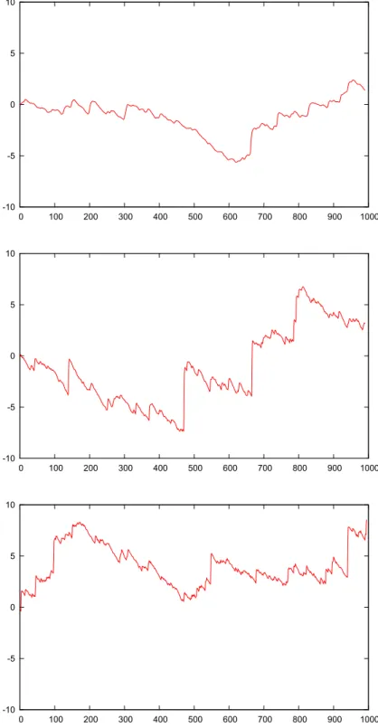
the number of particles exceeds N , only the N right-most particles are kept and the others are immediately killed. This gives a cloud of particles, moving to the right with a certain speed v_N ă 1 and fluctuating around its mean. See Figure 1 at the end of the introduction for simulations. The authors of [56] provide detailed quantitative heuristics to describe this behaviour:

(17)

1. Most of the time, the particles are in a meta-stable state. In this state, the diameter of the cloud of particles (also called the front ) is approximately log N , the empirical density of the particles proportional to e´x_{sinpπx{ log N q, and the system moves at a}

linear speed vcutoff “ 1 ´ π2{p2 log2N q. This is the description provided by the cutoff

approximation from [50] mentioned above.

2. This meta-stable state is perturbed from time to time by particles moving far to the right and thus spawning a large number of descendants, causing a shift of the front to the right after a relaxation time which is of the order of log2N . To make this precise, we fix a point in the bulk, for example the barycentre of the cloud of particles, and shift our coordinate system such that this point becomes its origin. Playing with the initial conditions of the FKPP equation with cutoff, the authors of [56] find that a particle moving up to the point log N ` x causes a shift of the front by

∆ “ log ´ 1 ` Ce x log3N ¯ ,

for some constant C ą 0. In particular, in order to have an effect on the position of the front, a particle has to reach a point near log N ` 3 log log N .

3. Assuming that such an event where a particle “escapes” to the point log N ` x happens with rate Ce´x_{, one sees that the time it takes for a particle to come close to log N `}

3 log log N (and thus causing shifts of the front) is of the order of log3N " log2N . 4. With this information, the full statistics of the position of the front (i.e. the speed v_N

and the cumulants of order n ě 2) are found to be vN´ vcutoff « π2 3 log log N log3N [n-th cumulant] t « π2n!ζpnq log3N , n ě 2, (2)

where ζ denotes the Riemann zeta-function.

In another paper [57], the same authors introduce a related model, called the exponential model. This is a BRW, where an individual at position x has an infinite number of descendants distributed according to a Poisson process of intensity ex´ydy. Again, at every step, only the N right-most particles are kept. This model has some translational invariance properties which render it exactly solvable. Besides asymptotics on the speed of this system and the fluctuations, the authors of [57] then show that the genealogy of this system converges to the celebrated Bolthausen–Sznitman coalescent7. This gives first insight into the fact that the genealogy of the N -BBM apparently converges to the same coalescent process, a fact that has been observed by numerical simulations [58, 59].

Despite (or because of) the simplicity of the N -BBM, it is very difficult to analyse it rigorously, because of the strong interaction between the particles, the impossibility to describe it exactly through differential equations and the fact that the shifts in the position of the system do not occur instantaneously but gradually over the fairly large timescale log2N . For this reason, there have been few rigorous results on the N -BBM or the N -BRW: Bérard and Gouéré [20] prove the log2N correction of the linear speed of N -BRW in the binary branching case, thereby showing the validity of the approximation by a deterministic travelling wave with cutoff. Durrett and Remenik [76] study the empirical distribution of N -BRW and show

7. The Bolthausen–Sznitman coalescent [40] is a process on the partitions of N, in which a proportion p of the blocks merge to a single one at rate p´2_{dp. See [26] and [24] for an introduction to coalescent processes.}

(18)

that it converges as N goes to infinity but time is fixed to a system of integro-differential equations with a moving boundary. Recently, Comets, Quastel and Ramírez [65] studied a particle system expected to exhibit similar behaviour than the exponential model and show in particular that its recentred position converges to a totally asymmetric Cauchy process.

In [56], the authors already had the idea of approximating the N -BBM by BBM with absorption at a linear barrier with the weakly subcritical slope v_N. This idea was then used with success in [20] for the proof of the cutoff-correction to the speed of the N -BRW, relying on a result [83] about the survival probability of BRW with absorption at such a barrier and a result by Pemantle about the number of nearly optimal paths in a binary tree [128]. In the same vein, Berestycki, Berestycki and Schweinsberg [23] studied the genealogy of BBM with absorption at this barrier and found that it converges at the log3N timescale to the Bolthausen–Sznitman coalescent, as predicted. In Chapter 2 of this thesis, we build upon their analysis in order to study the position of the N -BBM itself. The results that we prove are summarised in the following theorem, which confirms (2) (see Theorem 1.1 of Chapter 2 for a complete statement).

Theorem. Let XNptq denote the position of the rN {2s-th particle from the right in N -BBM.

Then under “good” initial conditions, the finite-dimensional distributions of the process `XN`t log3N

˘

´ vNt log3N

˘

tě0

converge weakly as N Ñ 8 to those of the Lévy process pLtqtě0 with

log EreiλpL1´L0q

s “ iλc ` π2 ż8

0

eiλx´ 1 ´ iλx1pxď1qΛpdxq,

where Λ is the image of the measure px´2₁

pxą0qqdx by the map x ÞÑ logp1 ` xq and c P R is

a constant depending only on the reproduction law qpkq.

In order to prove this result, we approximate the N -BBM by BBM with absorption at a random barrier instead of a linear one, a process which we call the B-BBM (“B” stands for “barrier”). This random barrier has the property that the number of individuals stays almost constant during a time of order log3N . We then couple the N -BBM with two variants of the B-BBM, the B5_{-BBM and the B}7_{-BBM, which in a certain sense bound the N -BBM from}

below and from above, respectively. For further details about the idea of the proof, we refer to Section 1 in Chapter 2.

Stable point processes occurring in branching Brownian motion. This paragraph describes the content of Chapter 3, which is independent from the first two and has nothing to do with selection. It concerns the extremal particles in BBM and BRW without selection, i.e. the particles which are near the right-most. The study of these particles has been initiated again by Brunet and Derrida [53], who gave arguments for the following fact: The point process formed by the particles of BBM at time t, shifted to the left by mptq “ t ´ 3{2 log t, converges as t Ñ 8 to a point process Z which has the “superposability” property: the union of Z translated by eα and Z1 _{translated by e}β _{has the same law as Z, where Z}1 _{is an}

independent copy of Z and eα` eβ “ 1. Moreover, they conjectured that this process, and possibly every process with the previous property, could be represented as a Poisson process with intensity e´x_{dx, decorated by an auxiliary point process D, i.e. each point ξ}

i of the

Poisson process is replaced by an independent copy of D translated by ξ_i.

In Chapter 3 we show that the “superposability” property has a classical interpretation in terms of stable point processes, pointed out to us by Ilya Molchanov, and the above-mentioned

(19)

representation is known in this field as the LePage series representation of a stable point process. We furthermore give a short proof of this representation using only the theory of infinitely divisible random measures. For the BBM and BRW, the convergence of the ex-tremal particles to such a process was proven by Arguin, Bovier, Kistler [10, 12, 11], Aïdékon, Berestycki, Brunet, Shi [4] and Madaule [114]. Kabluchko [98] also has an interesting result for BRW started with an infinite number of particles distributed with density e´cx_{dx, with}

c ą 1, which corresponds to travelling waves of speed larger than 1.

Conclusion and open problems

In this thesis, we have studied two models of branching Brownian motion with selection: the BBM with absorption at a linear barrier and the N -BBM. For the first model, we have given precise asymptotics on the number of absorbed particles in the case where the process gets extinct almost surely. For the second model, the study of which represents the major part of the thesis, we have shown that the recentred position of the particle system converges at the time-scale log3N to a Lévy process which is given explicitly. Finally, in the last chapter, we have pointed out a relation between the extremal particles of BBM and BRW and stable point processes.

The study of the N -BBM constitutes an important step in the understanding of general fluctuating wave fronts, whose phenomenology is believed to be the same in many cases [56]. Furthermore, it is a natural and intricate example of a selection mechanism for BBM and BRW and an intuitive model of a population under natural selection.

We have not considered models of BBM with selection with density-dependent selection, i.e. where particles get killed with a rate depending on the number of particles in their neigh-bourhood. This kind of selection is indeed the most relevant for applications in ecology and has appeared in the literature mostly as branching-coalescing particle systems (see for exam-ple [136, 135, 18, 125, 75, 15]), but also as systems with a continuous self-regulating density [137, 84]. However, although we have not directly considered this type of selection mecha-nism, the N -BBM is closely related to a particular case: Suppose particles perform BBM and furthermore coalesce at rate ε when they meet (i.e. let two particles coalesce when their intersection local time is equal to an independent exponential variable of parameter ε). Shiga [135] showed that this system is in duality with the noisy FKPP equation

B Btu “ 1 2 ˆ B Bx ˙2 u ` F puq `aεup1 ´ uq 9W , (3)

where 9W is space-time white noise. This equation admits “travelling wave” solutions whose wave speed equals the speed of the right-most particle of the branching-coalescing Brownian motion (BCBM) [121]. Now, following the argumentation in [121], the invariant measures of the BCBM are the Poisson process of intensity ε´1 _{and the configuration of no particles, the}

first being stable and the second unstable. Hence, if one looks at the right-most particles in the BCBM, they will ultimately form a wave-like profile with particles to the left of this wave distributed with a density ε´1_{. We have thus a similar picture than in the N -BBM, in that}

when particles get to the left of the front, they get killed quickly, in this case approximately with rate 1 instead of instantaneously. If ε is small, this does not make a difference because the typical diameter of the front goes to infinity as ε Ñ 0. It is therefore plausible that our results about the N -BBM can be transferred to the BCBM and thus to the noisy FKPP equation (3). Indeed, Mueller, Mytnik and Quastel [121] have showed that the wave speed of solutions to (3) is approximately vN (although they still have an error of Oplog log N { log3N q,

(20)

In what follows, we will outline several other open problems, mostly concerning the N -BBM.

Speed of the N -BBM. If the reproduction law satisfies qp0q “ 0, then the speed of the system is the constant v˚

N, such that XNptq{t Ñ vN˚ as t Ñ 8, where XNptq is again the

position of the rN {2s-th particle from the right in N -BBM. It has been shown [20] for the BRW with binary branching that this speed exists and it is not difficult to extend their proof to the BBM. Now, although our result about the position of the N -BBM describes quite precisely the fluctuations at the timescale log3N it tells us nothing about the behaviour of the system as time gets arbitrarily large. A priori, it could be possible that funny things happen at larger timescales, which lead to stronger fluctuations or a different speed of the system. In their proof [20] of the cutoff correction for the speed, Bérard and Gouéré had to consider in fact timescales up to log5N . It is therefore an open problem to prove that v˚

N “ vN` c1` oplog´3N q for some constant c1 P R and that the cumulants scale as in (2) as

t Ñ 8, which we conjecture to be true.

Empirical measure of the N -BBM. Let ν₀Nptq be the empirical measure of the particles at time t in N -BBM seen from the left-most particle. Durrett and Remenik [76] show (for BRW) that the process pN´1_νN

0 ptqqtPR is ergodic and therefore has an invariant probability

πN and furthermore converges as N Ñ 8 in law to a deterministic measure-valued process whose density with respect to Lebesgue measure solves a free boundary integro-differential equation. Our result on the N -BBM and those prior to our work [50, 56, 23] suggest that the πN should converge, as N Ñ 8, to the Dirac measure concentrated on the measure xe´x₁

xě0dx. If one was to prove this, the methods of [76], which are essentially based on

Gronwall’s inequality, would not directly apply, since they only work for timescales of at most log N . On the other hand, our technique of the coupling with BBM with absorption has fairly restrictive requirements on the initial configuration of the particles. A method of proof would therefore be to show that these requirements are met after a certain time for any initial configuration and then couple the processes.

The genealogy of the N -BBM. As mentioned above, the genealogy of the N -BBM is expected to converge at the timescale log3N to the Bolthausen–Sznitman coalescent as N goes to infinity. A step towards this conjecture is the article [23], in which the authors show that this convergence holds for BBM with absorption at a weakly subcritical barrier; it should be easy to extend their arguments for the B-BBM defined in Section 7 of Chapter 2. However, this would not be enough, since the monotone coupling we use to couple the N -BBM with the B-BBM (or rather its variants B5_{-BBM and B}7_{-BBM) does not preserve the genealogical}

structure of the process. More work is therefore required to prove the conjecture for the N -BBM.

The N -BRW. It should be possible to transfer the results obtained here for the N -BBM to the N -BRW, as long as the displacements have exponential right tails and the number of offspring of a particle has finite variance, say. Naturally, this would require a lot more work because of the lack of explicit expressions for the density of the particles; one can wonder whether this work would be worth it. However, it would be interesting to consider cases where one could get different behaviour than for the N -BBM, such as subexponentially decaying right tails of the displacements or models where particles have an infinite number of children, as in the exponential model. Another possible point of attack in the same direction would be to make rigorous for the N -BBM the findings in [55]. In that article, the authors

(21)

weight the process by an exponential weight eρRNptq_{, where R}

Nptq is the position of the

right-most particle at time t, and obtain thus a one-parameter family of coalescent processes as genealogies.

Superprocesses. If one considers N independent BBMs with weakly supercritical repro-duction (i.e. m “ a{N for some constant a ą 0), gives the mass N´1 _{to each individual and}

rescales time by N and space by N´1_{, then one obtains in the limit a (supercritical)}

superpro-cess, such as the Dawson–Watanabe process in the case that the variance of the reproduction law is finite (see [77] for a gentle introduction to superprocesses). One may wonder whether the results obtained in this thesis have analogues in that setting. This is true for the results obtained in Chapter 1, as shown in [110], in which the authors indeed transfer the results di-rectly via the so-called backbone decomposition of the superprocess [109]. As for an analogue of the N -BBM: one could consider a similar model of a superprocess whose mass is kept below N by stripping off some mass to the left as soon as the total mass exceeds N . It is possible that this process then exhibits similar fluctuations, which could again be related to those of the N -BBM by the backbone decomposition.

(22)

-10 -5 0 5 10 0 100 200 300 400 500 600 700 800 900 1000 -10 -5 0 5 10 0 100 200 300 400 500 600 700 800 900 1000 -10 -5 0 5 10 0 100 200 300 400 500 600 700 800 900 1000

Figure 1: Simulation of the N -BRW with (from top to bottom) N “ 1010, N “ 1030 and N “ 1060particles (particles branch at each time step with probability 0.05 into two and jump one step to the right with probability 0.25). The graphs show the barycentre of the particles recentred roughly around v_Nt (because of the slow convergence, small linear correction terms had to be added in order to fit the graphs into the rectangles). The horizontal axis shows time (at the scale log3N ), the vertical axis shows the position of the barycentre (without rescaling).

(23)

(24)

The number of absorbed individuals

in branching Brownian motion with a

barrier

This chapter is based on the article [115].

1 Introduction

We recall the definition of branching Brownian motion mentioned already in the intro-ductory chapter: Starting with an initial individual sitting at the origin of the real line, this individual moves according to a 1-dimensional Brownian motion with drift c until an inde-pendent exponentially distributed time with rate 1. At that moment it dies and produces L (identical) offspring, L being a random variable taking values in the non-negative integers with P pL “ 1q “ 0. Starting from the position at which its parent has died, each child repeats this process, all independently of one another and of their parent. For a rigorous definition of this process, see for example [94] or [61].

We assume that m “ ErLs ´ 1 P p0, 8q, which means that the process is supercritical. At position x ą 0, we add an absorbing barrier, i.e. individuals hitting the barrier are instantly killed without producing offspring. Kesten proved [102] that this process becomes extinct almost surely if and only if the drift c ě c0 “

?

2m (he actually needed ErL2s ă 8 for the “only if” part, but we are going to prove that the statement holds in general). Neveu [123] showed that the process Z “ pZxqxě0 is a continuous-time Galton–Watson process of finite

expectation, but with ErZxlog`Zxs “ 8 for every x ą 0, if c “ c0.

Let N “ t1, 2, 3, . . .u and N0 “ t0u Y N. Define the infinitesimal transition rates (see [14],

p. 104, Equation (6) or [89], p. 95) qn“ lim

xÓ0

1

xP pZx“ nq, n P N0zt1u. We propose a refinement of Neveu’s result:

Theorem 1.1. Let c “ c0 and assume that ErLplog Lq2s ă 8. Then we have as n Ñ 8, 8 ÿ k“n qk„ c0 nplog nq2 and P pZx ą nq „ c0xec0x

nplog nq2 for each x ą 0.

The heavy tail of Z_x suggests that its generating function is amenable to singularity analysis in the sense of [81]. This is in fact the case in both the critical and subcritical cases if we impose a stronger condition upon the offspring distribution and leads to the next theorem.

(25)

Define f psq “ ErsLs the generating function of the offspring distribution. Denote by δ the span of L ´ 1, i.e. the greatest positive integer, such that L ´ 1 is concentrated on δZ. Let λcď λc be the two roots of the quadratic equation λ2´ 2cλ ` c20 “ 0 and denote by d “ λcλc

the ratio of the two roots. Note that c “ c0 if and only if λc“ λc if and only if d “ 1.

Theorem 1.2. Assume that the law of L admits exponential moments, i.e. that the radius of convergence of the power series ErsLs is greater than 1.

´ In the critical speed area pc “ c0q, as n Ñ 8,

qδn`1„

c0

δn2_{plog nq}2 and P pZx “ δn ` 1q „

c0xec0x

δn2_{plog nq}2 for each x ą 0.

´ In the subcritical speed area pc ą c0q there exists a constant K “ Kpc, f q ą 0, such that,

as n Ñ 8, qδn`1 „ K nd`1 and P pZx“ δn ` 1q „ eλcx´ eλcx λc´ λc K nd`1 for each x ą 0.

Furthermore, q_δn`k “ P pZx“ δn ` kq “ 0 for all n P Z and k P t2, . . . , δu.

Remark 1.3. The idea of using singularity analysis for the study of Zx comes from Robin

Pemantle’s (unfinished) manuscript [127] about branching random walks with Bernoulli re-production.

Remark 1.4. Since the coefficients of the power series ErsLs are real and non-negative, Pring-sheim’s theorem (see e.g. [82], Theorem IV.6, p. 240) entails that the assumption in Theorem 1.2 is verified if and only if f psq is analytic at 1.

Remark 1.5. Let β ą 0 and σ ą 0. We consider a more general branching Brownian motion with branching rate given by β and the drift and variance of the Brownian motion given by c and σ2, respectively. Call this process the pβ, c, σq-BBM (the reproduction is still governed by the law of L, which is fixed). In this terminology, the process described at the beginning of this section is the p1, c, 1q-BBM. The pβ, c, σq-BBM can be obtained from p1, c{pσ?βq, 1q-BBM by rescaling time by a factor β and space by a factor σ{?β. Therefore, if we add an absorbing barrier at the point x ą 0, the pβ, c, σq-BBM gets extinct a.s. if and only if c ě c0“ σ

? 2βm. Moreover, if we denote by Zxpβ,c,σq the number of particles absorbed at x, we obtain that

pZxpβ,c,σqqxě0 and pZp1,c{pσ ?

βq,1q

x?β{σ qxě0 are equal in law.

In particular, if we denote the infinitesimal transition rates of pZxpβ,c,σqqxě0 by qpβ,c,σqn , for

n P N0zt1u, then we have

q_npβ,c,σq“ lim xÓ0 1 xP ´ Z_xpβ,c,σq“ n ¯ “ ? β σ limxÓ0 σ x?βP ´ Zp1,c{pσ ? βq,1q x?β{σ “ n ¯ “ ? β σ q p1,c{pσ?βq,1q n .

One therefore easily checks that the statements of Theorems 1.1 and 1.2 are still valid for arbitrary β ą 0 and σ ą 0, provided that one replaces the constants c0, λc, λc, K by c0{σ2,

λc{σ2, λc{σ2, ? β σ Kpc{pσ ? βq, f q, respectively.

The content of the paper is organised as follows: In Section 2 we derive some preliminary results by probabilistic means. In Section 3, we recall a known relation between Z_x and the so-called Fisher–Kolmogorov–Petrovskii–Piskounov (FKPP) equation. Section 4 is devoted to the proof of Theorem 1.1, which draws on a Tauberian theorem and known asymptotics of travelling wave solutions to the FKPP equation. In Section 5 we review results about complex differential equations, singularity analysis of generating functions and continuous-time Galton–Watson processes. Those are needed for the proof of Theorem 1.2, which is done in Section 6.

(26)

2 First results by probabilistic methods

The goal of this section is to prove

Proposition 2.1. Assume c ą c0 and ErL2s ă 8. There exists a constant C “ Cpx, c, Lq ą

0, such that

P pZx ą nq ě

C

nd for large n.

This result is needed to assure that the constant K in Theorem 1.2 is non-zero. It is independent from Sections 3 and 4 and in particular from Theorem 1.1. Its proof is entirely probabilistic and follows closely [2].

2.1 Notation and preliminary remarks

Our notation borrows from [108]. An individual is an element in the space of Ulam–Harris labels

U “ ď

nPN0

Nn,

which is endowed with the ordering relations ĺ and ă defined by

u ĺ v ðñ Dw P U : v “ uw and u ă v ðñ u ĺ v and u ‰ v.

The space of Galton–Watson trees is the space of subsets t Ă U , such that ∅ P t, v P t if v ă u and u P t and for every u there is a number Lu P N0, such that for all j P N, uj P t if

and only if j ď Lu. Thus, Lu is the number of children of the individual u.

Branching Brownian motion is defined on the filtered probability space pT ,F , pFtq, P q.

Here, T is the space of Galton–Watson trees with each individual u P t having a mark pζu, Xuq P R` ˆ DpR`, R Y t∆uq, where ∆ is a cemetery symbol and DpR`, R Y t∆uq

denotes the Skorokhod space of cadlag functions from R` _{to R Y t∆u. Here, ζ}

u denotes the

life length and Xuptq the position of u at time t, or of its ancestor that was alive at time t.

More precisely, for v P t, let dv “

ř

wĺvζw denote the time of death and bv “ dv ´ ζv the

time of birth of v. Then X_uptq “ ∆ for t ě du and if v ĺ u is such that t P rbv, dvq, then

Xuptq “ Xvptq.

The sigma-field F_tcontains all the information up to time t, and F “ σ `Ť_tě0F_t˘. Let y, c P R and L be some random variable taking values in N0zt1u. P “ Py,c,L is the

unique probability measure, such that, starting with a single individual at the point y, ´ each individual moves according to a Brownian motion with drift c until an independent

time ζ_u following an exponential distribution with parameter 1.

´ At the time ζu the individual dies and leaves Lu offspring at the position where it has

died, with L_u being an independent copy of L.

´ Each child of u repeats this process, all independently of one another and of the past of the process.

Note that often c and L are regarded as fixed and y as variable. In this case, the notation Py is used. In the same way, expectation with respect to P is denoted by E or Ey.

A common technique in branching processes since [113] is to enhance the space T by selecting an infinite genealogical line of descent from the ancestor ∅, called the spine. More precisely, if T P T and t its underlying Galton–Watson tree, then ξ “ pξ0, ξ1, ξ2, . . .q P UN0 is

a spine of T if ξ0 “ ∅ and for every n P N0, ξn`1 is a child of ξn in t. This gives the space

r

(27)

of marked trees with spine and the sigma-fields ĂF and ĂF_t. Note that if pT, ξq P rT , then T is necessarily infinite.

Assume from now on that m “ ErLs ´ 1 P p0, 8q. Let Nt be the set of individuals alive

at time t. Note that every ĂFt-measurable function f : rT Ñ R admits a representation

f pT, ξq “ ÿ

uPNt

fupT q1uPξ,

where fu is anFt-measurable function for every u P U . We can therefore define a measure rP

on p rT , ĂF , p ĂF_tqq by ż r T f d rP “ e´mt ż T ÿ uPNt fupT qP pdT q. (2.1)

It is known [108] that this definition is sound and that rP is actually a probability measure with the following properties:

´ Under rP , the individuals on the spine move according to Brownian motion with drift c and die at an accelerated rate m ` 1, independent of the motion.

´ When an individual on the spine dies, it leaves a random number of offspring at the point where it has died, this number following the size-biased distribution of L. In other words, let rL be a random variable with Erf prLqs “ Erf pLqL{pm ` 1qs for every positive measurable function f . Then the number of offspring is an independent copy of rL. ´ Amongst those offspring, the next individual on the spine is chosen uniformly. This

individual repeats the behaviour of its parent.

´ The other offspring initiate branching Brownian motions according to the law P . Seen as an equation rather than a definition, (2.1) also goes by the name of “many-to-one lemma”.

2.2 Branching Brownian motion with two barriers

We recall the notation Py from the previous subsection for the law of branching Brownian motion started at y P R and Ey the expectation with respect to Py. Recall the definition of

r

P and define rPy and rEy analogously.

Let a, b P R such that y P pa, bq. Let τ “ τa,b be the (random) set of those individuals

whose paths enter p´8, as Y rb, 8q and all of whose ancestors’ paths have stayed inside pa, bq. For u P τ we denote by τ puq the first exit time from pa, bq by u’s path, i.e.

τ puq “ inftt ě 0 : Xuptq R pa, bqu “ mintt ě 0 : Xuptq P ta, buu,

and set τ puq “ 8 for u R τ . The random set τ is an (optional) stopping line in the sense of [61].

For u P τ , define Xupτ q “ Xupτ puqq. Denote by Za,b the number of individuals leaving

the interval pa, bq at the point a, i.e. Za,b“

ÿ

uPτ

1Xupτ q“a.

Lemma 2.2. Assume |c| ą c0 and define ρ “

a c2_{´ c}2 0. Then EyrZa,bs “ ecpa´yq sinhppb ´ yqρq sinhppb ´ aqρq.

(28)

If, furthermore, V “ ErLpL ´ 1qs ă 8, then EyrZa,b2 s “ 2V ecpa´yq ρ sinh3ppb ´ aqρq ” sinhppb ´ yqρq ży a

ecpa´rqsinh2ppb ´ rqρq sinhppr ´ aqρq dr

` sinhppy ´ aqρq żb y ecpa´rqsinh3ppb ´ rqρq dr ı ` EyrZa,bs.

Proof. On the space rT of marked trees with spine, define the random variable I by I “ i if ξi P τ and I “ 8 otherwise. For an event A and a random variable Y write ErY, As instead

of ErY 1As. Then EyrZa,bs “ Ey ” ÿ uPτ 1_{Xupτ q“a} ı “ rEyremτ pξIq, I ă 8, XξIpτ q “ as

by the many-to-one lemma extended to optional stopping lines (see [33], Lemma 14.1 for a discrete version). But since the spine follows Brownian motion with drift c, we have I ă 8,

r

P -a.s. and the above quantity is therefore equal to Wy,cremT, BT “ as,

where Wy,c is the law of standard Brownian motion with drift c started at y, pBtqtě0 the

canonical process and T “ Ta,b the first exit time from pa, bq of Bt. By Girsanov’s theorem,

and recalling that m “ c2₀{2, this is equal to

WyrecpBT´yq´12pc2´c20qT_{, B}

T “ as,

where Wy “ Wy,0. Evaluating this expression ([41], p. 212, Formula 1.3.0.5) gives the first equality.

For u P U , let Θu be the operator that maps a tree in T to its sub-tree rooted in u. Denote

further by C_u the set of u’s children, i.e. C_u “ tuk : 1 ď k ď Luu. Then note that for each

u P τ we have Za,b“ 1 ` ÿ vău ÿ wPCv włu Za,b˝ Θw, hence EyrZa,b2 s “ Ey ” ÿ uPτ

1Xupτ q“aZa,b

ı “ EyrZa,bs ` rPy « emτ pξIq ÿ văξI ÿ wPLv włξI Za,b˝ Θw, XξIpτ q “ a ff . (2.2)

Define the σ-algebras

G “ σpXξIptq; t ě 0q,

H “ G _ σpζv; v ă ξIq,

I “H _ σpξ, I, pLv; v ă ξIqq,

such that G contains the information about the path of the spine up to the individual that quits pa, bq first,H adds to G the information about the fission times on the spine and I adds to H the information about the individuals of the spine and the number of their children.

(29)

Now, conditioning on I and using the strong branching property, the second term in the last line of (2.2) is equal to r Py « emτ pξIq ÿ văξI

pLv´ 1qEXvpdv´qrZa,bs, XξIpτ q “ a

ff

(recall that dv is the time of death of v). Conditioning on H and noting the fact that Lv

follows the size-biased law of L for an individual v on the spine, yields

r Py « emτ pξIq ÿ văξI V m ` 1E X_ξIpdvq rZa,bs, XξIpτ q “ a ff .

Finally, since under rP the fission times on the spine form a Poisson process of intensity m ` 1, conditioning on G and applying Girsanov’s theorem yields

Wy „ ecpBT´yq´1₂ρ2T żT 0 V EBtrZa,bs dt, BT “ a  “ V ecpa´yq żb a ErrZa,bsWy ” e´12ρ 2_T Lr_T, BT “ a ı dr,

where Lr_T is the local time of pBtq at the time T and the point r. The last expression can be

evaluated explicitly ([41], p. 215, Formula 1.3.3.8) and gives the desired equality.

Corollary 2.3. Under the assumptions of Lemma 2.2, for each b ą 0 there are positive constants C_bp1q, C_bp2q, such that as a Ñ ´8,

a) E0rZa,bs „ C_bp1qepc`ρqa, b) if c ą c0, E0rZa,b2 s „ C p2q b epc`ρqa and c) if c ă ´c0, E0rZa,b2 s „ C p2q b e2pc`ρqa.

The following result is well known and is only included for completeness. We emphasize that the only moment assumption here is m “ ErLs ´ 1 P p0, 8q. Recall that Zx denotes the

number of particles absorbed at x of a BBM started at the origin. For |c| ě c0, define λc to

be the smaller root of λ2´ 2cλ ` c20, thus λc“ c ´

a c2_{´ c}2 0. Lemma 2.4. Let x ą 0. ´ If |c| ě c0, then ErZxs “ eλcx. ´ If |c| ă c0, then ErZxs “ `8.

Proof. We proceed similarly to the first part of Lemma 2.2. Define the (optional) stopping line τ of the individuals whose paths enter rx, 8q and all of whose ancestors’ paths have stayed inside p´8, xq. Define I as in the proof of Lemma 2.2. By the stopping line version of the many-to-one lemma we have

ErZxs “ Er

ÿ

uPτ

1s “ rEremτ pξIq, I ă 8s.

By Girsanov’s theorem, this equals

W recx´12pc 2_´c2

0qTx_{, T}_x_{ă 8s,}

where W is the law of standard Brownian motion started at 0 and Tx is the first hitting time

(30)

2.3 Proof of Proposition 2.1

By hypothesis, c ą c0, ErL2s ă 8 and the BBM starts at the origin. Let x ą 0 and let

τ “ τx be the stopping line of those individuals hitting the point x for the first time. Then

Zx“ |τx|.

Let a ă 0 and n P N. By the strong branching property,

P0pZxą nq ě P0pZxą n | Za,x ě 1qP0pZa,x ě 1q ě PapZx ą nqP0pZa,xě 1q.

If P_´0 denotes the law of branching Brownian motion started at the point 0 with drift ´c, then

PapZxą nq “ P´0pZa´xą nq ě P´0pZa´x,1ą nq.

In order to bound this quantity, we choose a “ an in such a way that n “ 1₂E´0rZan´x,1s. By

Corollary 2.3 a), c) (applied with drift ´c) and the Paley–Zygmund inequality, there is then a constant C1 ą 0, such that

P_´0pZan´x,1 ą nq ě

1 4

E0_´rZan´x,1s2

E_´0rZ_an´x,12 s ě C1 for large n.

Furthermore, by Corollary 2.3 a) (applied with drift ´c), we have 1 2C p1q 1 e ´λcpan´xq „ n, as n Ñ 8,

and therefore a_n“ ´p1{λcq log n ` Op1q. Again by the Paley–Zygmund inequality and

Corol-lary 2.3 a), b) (applied with drift c), there exists C₂ą 0, such that for large n,

P0pZan,xě 1q “ P0pZan,xą 0q ě E0rZan,xs2 E0_rZ2 an,xs ě pC p1q x q2 2Cxp2q eλcan ě C2 nd.

This proves the proposition with C “ C1C2.

3 The FKPP equation

As was already observed by Neveu [123], the translational invariance of Brownian motion and the strong branching property immediately imply that Z “ pZxqxě0 is a homogeneous

continuous-time Galton–Watson process (for an overview to these processes, see [14], Chap-ter III or [89], ChapChap-ter V). There is therefore an infinitesimal generating function

apsq “ α ˜ 8 ÿ n“0 pnsn´ s ¸ , α ą 0, p1“ 0, (3.1)

associated to it. It is a strictly convex function on r0, 1s, with ap0q ě 0 and ap1q ď 0. Its probabilistic interpretation is

α “ lim

xÑ0 1

xP pZx ‰ 1q and pn“ lim_xÑ0P pZx“ n|Zx ‰ 1q,

hence q_n “ αpn for n P N0zt1u. Note that with no further conditions on c and L, the sum

ř

ně0pn need not necessarily be 1, i.e. the rate αp8, where p8 “ 1 ´

ř

ně0pn, with which

(31)

We further define Fxpsq “ ErsZxs, which is linked to apsq by Kolmogorov’s forward and backward equations ([14], p. 106 or [89], p. 102): B BxFxpsq “ apsq B BsFxpsq (forward equation) (3.2) B

BxFxpsq “ arFxpsqs (backward equation) (3.3)

The forward equation implies that if ap1q “ 0 and φpxq “ ErZxs “ _BsBFxp1´q, then φ1pxq “

a1_{p1qφpxq, whence ErZ} xs “ ea

1_p1qx

. On the other hand, if ap1q ă 0, then the process jumps to 8 with positive rate, hence ErZxs “ 8 for all x ą 0.

The next lemma is an extension of a result which is stated, but not proven, in [123], Equation (1.1). According to Neveu, it is due to A. Joffe. To the knowledge of the author, no proof of this result exists in the current literature, which is why we prove it here.

Lemma 3.1. Let pYtqtě0 be a homogeneous Galton–Watson process started at 1, which may

explode and may jump to `8 with positive rate. Let upsq be its infinitesimal generating function and Ftpsq “ ErsYts. Let q be the smallest zero of upsq in r0, 1s.

1. If q ă 1, then there exists t´ P R Y t´8u and a strictly decreasing smooth function

ψ´ : pt´, `8q Ñ pq, 1q with limtÑt´ψ´ptq “ 1 and limtÑ8ψ´ptq “ q, such that on

pq, 1q we have u “ ψ´1 ˝ ψ ´1

´ , Ftpsq “ ψ´pψ´1´ psq ` tq.

2. If q ą 0, then there exists t` P R Y t´8u and a strictly increasing smooth function

ψ` : pt`, `8q Ñ p0, qq with limtÑt`ψ`ptq “ 0 and limtÑ8ψ`ptq “ q, such that on

p0, qq we have u “ ψ`1 ˝ ψ ´1

` , Ftpsq “ ψ`pψ´1` psq ` tq.

The functions ψ_´ and ψ_` are unique up to translation. Moreover, the following statements are equivalent: ´ For all t ą 0, Ytă 8 a.s.

´ q “ 1 or t´“ ´8.

Proof. We first note that upsq ą 0 on p0, qq and upsq ă 0 on pq, 1q, since upsq is strictly convex, up0q ě 0 and up1q ď 0. Since F0psq “ s, Kolmogorov’s forward equation (3.2) implies

that F_tpsq is strictly increasing in t for s P p0, qq and strictly decreasing in t for s P pq, 1q. The backward equation (3.3) implies that Ftpsq converges to q as t Ñ 8 for every s P r0, 1q.

Repeated application of (3.3) yields that Ftpsq is a smooth function of t for every s P r0, 1s.

Now assume that q ă 1. For n P N set sn “ 1 ´ 2´np1 ´ qq, such that q ă s1 ă 1,

snă sn`1 and snÑ 1 as n Ñ 8. Set t1 “ 0 and define tn recursively by

tn`1 “ tn´ t1, where t1 ą 0 is such that Ft1ps_n`1q “ s_n.

Then ptnqnPN is a decreasing sequence and thus has a limit t´P R Y t´8u. We now define

for t P pt´, `8q,

ψ´ptq “ Ft´tnpsnq, if t ě tn.

The function ψ´ is well defined, since for every n P N and t ě tn,

Ft´tnpsnq “ Ft´tnpFtn´tn`1psn`1qq “ Ft´tn`1psn`1q,

by the branching property. The same argument shows us that if s P pq, 1q, sn ą s and t1 ą 0

such that F_t1ps_nq “ s, then F_tpsq “ F_t`t1ps_nq “ ψ_´pt ` t1` t_nq for all t ě 0. In particular,

ψ´pt1` tnq “ s, hence Ftpsq “ ψ´pψ´1´ psq ` tq. The backward equation (3.3) now gives

upsq “ B BtFtpsqˇˇt“0“ ψ 1 ´pψ ´1 ´ psqq.

(32)

The second part concerning ψ`is proven completely analogously. Uniqueness up to translation

of ψ_´ and ψ_` is obvious from the requirement ψpψ´1

psq ` tq “ Ftpsq, where ψ is either ψ´

or ψ`.

For the last statement, note that P pYt ă 8q “ 1 for all t ą 0 if and only if Ftp1´q “ 1

for all t ą 0. But this is the case exactly if q “ 1 or t´“ ´8.

The following proposition shows that the functions ψ´ and ψ` corresponding to pZxqxě0

are so-called travelling wave solutions of a reaction-diffusion equation called the Fisher–Kolmo-gorov–Petrovskii–Piskounov (FKPP) equation. This should not be regarded as a new result, since Neveu ([123], Proposition 3) proved it already for the case c ě c0 and L “ 2 a.s. (dyadic

branching). However, his proof relied on a path decomposition result for Brownian motion, whereas we show that it follows from simple renewal argument valid for branching diffusions in general.

Recall that f psq “ ErsLs denotes the generating function of L. Let q1 be the unique fixed point of f in r0, 1q (which exists, since f1

p1q “ m ` 1 ą 1), and let q be the smallest zero of apsq in r0, 1s.

Proposition 3.2. Assume c P R. The functions ψ´ and ψ` from Lemma 3.1 corresponding

to pZxqxě0 are solutions to the following differential equation on pt´, `8q and pt`, `8q,

respectively.

1 2ψ

2

´ cψ1 “ ψ ´ f ˝ ψ. (3.4)

Moreover, we have the following three cases:

1. If c ě c0, then q “ q1, t´“ ´8, ap1q “ 0, a1p1q “ λc, ErZxs “ eλcx for all x ą 0.

2. If |c| ă c0, then q “ q1, t´P R, ap1q ă 0, a1p1q “ 2c, P pZx“ 8q ą 0 for all x ą 0.

3. If c ď ´c0, then q “ 1, ap1q “ 0, a1p1q “ λc, ErZxs “ eλcx for all x ą 0.

Proof. Let s P p0, 1q and define the function ψspxq “ Fxpsq “ ErsZxs for x ě 0. By

sym-metry, Z_x has the same law as the number of individuals N absorbed at the origin in a branching Brownian motion started at x and with drift ´c. By a standard renewal argument (Lemma 7.1), the function ψs is therefore a solution of (3.4) on p0, 8q with ψsp0`q “ s. This

proves the first statement, in view of the representation of F_x in terms of ψ´ and ψ` given

by Lemma 3.1.

Let s P p0, 1qztqu and let ψpsq “ ψ´psq if s ą q and ψpsq “ ψ`psq otherwise. By (3.4),

a1psq “ ψ 2 ˝ ψ´1psq ψ1_{˝ ψ}´1_psq “ 2c ` 2 ψ ˝ ψ´1 psq ´ f ˝ ψ ˝ ψ´1psq ψ1_{˝ ψ}´1_psq “ 2c ` 2 s ´ f psq apsq , whence, by convexity, a1psqapsq “ 2capsq ` 2ps ´ f psqq, s P r0, 1s. (3.5)

Assume |c| ě c0. By Lemma 2.4, ErZxs “ eλcx, hence ap1q “ 0 and a1p1q “ λc, in

particular, a1_{p1q ą 0 for c ě c}

0 and a1p1q ă 0 for c ď ´c0. By convexity, q ă 1 for c ě c0 and

q “ 1 for c ď ´c0. The last statement of Lemma 3.1 now implies that t´“ ´8 if c ě c0.

Now assume |c| ă c0. By Lemma 2.4, ErZxs “ `8 for all x ą 0, hence either ap1q ă 0

or ap1q “ 0 and a1_{p1q “ `8, in particular, q ă 1 by convexity. However, if ap1q “ 0, then}

by (3.5), a1_{p1q “ 2c ´ 2m{a}1_{p1q, whence the second case cannot occur. Thus, ap1q ă 0 and}

a1

p1q “ 2c by (3.5).

It remains to show that q “ q1 _{if q ă 1. Assume q ‰ q}1_{. Then apq}1

q ‰ 0 by the (strict) convexity of a and a1_pq1_{q “ 2c by (3.5). In particular, a}1_pq1_{q ě a}1_{p1q, which is a contradiction}

(33)

4 Proof of Theorem 1.1

We have c “ c0 by hypothesis. Let ψ´be the travelling wave from Proposition 3.2, which

is defined on R, since t_´“ ´8. Let φpxq “ 1´ψ´p´xq, such that φp´8q “ 1´q, φp`8q “ 0

and 1 2φ 2 pxq ` c0φ1pxq “ f p1 ´ φpxqq ´ p1 ´ φpxqq, (4.1) by (3.4). Furthermore, ap1 ´ sq “ φ1 pφ´1psqq and Fxp1 ´ sq “ 1 ´ φpφ´1psq ´ xq.

Under the hypothesis ErLplog Lq2s ă 8, it is known [143] that there exists K P p0, 8q, such that φpxq „ Kxe´c0x _{as x Ñ 8. Since ap1q “ 0 and a}1_{p1q “ c}

0 by Proposition 3.2, this entails that φ1 pxq “ ap1 ´ φpxqq „ ć0Kxeć0x, as x Ñ 8. Set ϕ₁ “ φ1 and ϕ₂ “ φ. By (4.1), d dx ˆϕ1pxq ϕ2pxq ˙ “ˆφ 2_pxq φ1_pxq ˙ “ ˆ ´2c0φ1pxq ` 2rf p1 ´ φpxqq ´ p1 ´ φpxqqs φ1_pxq ˙ . Setting gpsq “ c2₀s ` 2rf p1 ´ sq ´ p1 ´ sqs “ 2rf1 p1qs ` f p1 ´ sq ´ 1s, this gives d dx ˆϕ1pxq ϕ2pxq ˙ “ Mˆϕ1pxq ϕ2pxq ˙ `ˆgpϕ2pxqq 0 ˙ , with M “ ˆ ´2c0 ć20 1 0 ˙ . (4.2)

The Jordan decomposition of M is given by

J “ A´1M A “ ˆ ć0 1 0 ć0 ˙ , A “ ˆ ć0 1 ´ c0 1 1 ˙ . (4.3) Settingˆϕ1 ϕ2 ˙ = Aˆξ1 ξ2 ˙ , we get with ξ “ˆξ1 ξ2 ˙ : ξ1pxq “ J ξpxq ` ˆ ´gpφpxqq gpφpxqq ˙ , which, in integrated form, becomes

ξpxq “ exJξp0q ` exJ żx 0 eýJ ˆ ´gpφpyqq gpφpyqq ˙ dy. (4.4) Note that exJ “ê ć0x _xeć0x 0 eć0x ˙ . (4.5)

With the above asymptotic of φ, the integral ş8₀ ec0ygpφpyqq dy is finite by Theorem B of [36] (see also Theorem 8.1.8 in [37]). Equations (4.4) and (4.5) now imply that

ξ2pxq „ e´c0x ´ ξ2p0q ` ż8 0 ec0ygpφpyqq dy ¯ , and pξ1` ξ2qpxq „ xe´c0x ´ ξ2p0q ` ż8 0 ec0ygpφpyqq dy ¯ , and since φ “ ξ1` ξ2 and ξ2 “ φ1` c0φ, this gives

Branching Brownian motion with selection

HAL Id: tel-00741368

https://tel.archives-ouvertes.fr/tel-00741368

Pascal Maillard

To cite this version:

École Doctorale Paris Centre

Thèse de doctorat

Discipline : Mathématiques

Pascal Maillard

Mouvement brownien branchant avec sélection

(Branching Brownian motion with selection)

dirigée par Zhan Shi

Rapporteurs :

M. Andreas Kyprianou University of Bath

M. Ofer Zeitouni

University of Minnesota

& Weizmann Institute of Science

Soutenue le 11 octobre 2012 devant le jury composé de :

M

Brigitte Chauvin

Université de Versailles

examinatrice

M. Francis Comets

Université Paris 7

examinateur

M. Bernard Derrida

Université Paris 6 et ENS examinateur

M. Yueyun Hu

Université Paris 13

examinateur

M. Andreas Kyprianou University of Bath

rapporteur

Remerciements

Résumé

Branching Brownian motion with selection

Abstract

Contents

Introduction

Results

Conclusion and open problems

The number of absorbed individuals

in branching Brownian motion with a

barrier

1

Introduction

2

First results by probabilistic methods

3

The FKPP equation

4

Proof of Theorem 1.1

_{Brigitte Chauvin}