HAL Id: hal-00155085
https://hal.archives-ouvertes.fr/hal-00155085
Submitted on 15 Jun 2007HAL is a multi-disciplinary open access archive for the deposit and dissemination of sci-entific research documents, whether they are pub-lished or not. The documents may come from teaching and research institutions in France or abroad, or from public or private research centers.
L’archive ouverte pluridisciplinaire HAL, est destinée au dépôt et à la diffusion de documents scientifiques de niveau recherche, publiés ou non, émanant des établissements d’enseignement et de recherche français ou étrangers, des laboratoires publics ou privés.
Oceanic Rossby waves acting as a ”hay rake” for
ecosystem floating by-products
Yves Dandonneau, Andres Vega, Hubert Loisel, Yves Du Penhoat, Christophe
E. Menkès
To cite this version:
Yves Dandonneau, Andres Vega, Hubert Loisel, Yves Du Penhoat, Christophe E. Menkès. Oceanic Rossby waves acting as a ”hay rake” for ecosystem floating by-products. Science, American Association for the Advancement of Science, 2003, 302 (5650), pp.1548-1551. �10.1126/science.1090729�. �hal-00155085�
Oceanic Rossby waves acting as
a “hay rake” for
ecosystem floating by-products
Yves Dandonneau1, Andres Vega2, Hubert Loisel3, Yves du Penhoat2
and Christophe Menkes1
1 IRD, IPSL/Laboratoire d’Océanographie Dynamique et de Climatologie, 75252 Paris 05,
France
2 IRD, Laboratoire d’Etudes en Géophysique et Océanographie Spatiale, Toulouse, France 3 MREN- Université du Littoral - Côte d'Opale, UMR 8013, Wimereux, France
Recent satellite observations of Rossby waves and chlorophyll anomalies propagating in subtropical gyres have suggested that wave-induced upwelling could stimulate photosynthesis. Instead, we show that chlorophyll maxima are located in abnormally warm water, in Rossby wave-induced convergences. This excludes inputs of nutrients from deeper water. We argue that the sea color anomalies are not caused by chlorophyll but by floating particles evolved from the ecosystem, and accumulated by Rossby waves, acting as “marine hay rakes”, in convergence zones. Such processes may be determinant for the distribution of living organisms in oligotrophic areas.
Subtropical anticyclonic gyres represent about 40% of the world ocean and have very low nutrient and chlorophyll levels, and permanently deep pycnoclines and nutriclines. In these oligotrophic areas, respiration balances, and sometimes exceeds photosynthesis (1). Primary production is mostly supported by the regeneration of nutrients by the microbial loop while export production remains low all the year round. Yet, export production estimates based on seasonal geochemical budgets, while low, is not entirely accounted for by the mean upwelling of nutrients to the photic layer (2, 3). It has thus been suggested that eddy induced nutrient pumping to the photic layer (3) may account for the remainder of export production.
Recently, large scale propagations of Rossby waves (RWs) from sea level and concurrent ocean color signals have been observed in all subtropical gyres. Nutrient pumping into the photic layer has been proposed as the mechanism by which RWs could increase chlorophyll concentration in these oligotrophic areas (4, 5). Thus, RWs would act like a “rototiller” by lifting nutrients continuously to the photic layer as they propagate (6), accounting for some of the missing production in the subtropical gyres. However, the coupling between the dynamics and chlorophyll anomalies has not been elucidated. Using satellite data, we examine here the relations
2 between RWs and chlorophyll concentration in the south Pacific subtropical gyre. We focus on the area 16°S - 22°S / 120° W - 80° W where RWs have a marked signature.
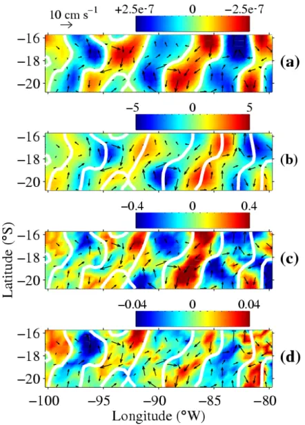
Figure 1. May 2000 maps of monthly band-passed satellite observations in the south Pacific subtropical gyre. (a) convergence (= negative divergence), (b) SLAs, (c) SSTAs and (d) ChlAs. Black arrows are geostrophic currents (10). Red (blue) represents positive (negative)
convergences, SLAs, SSTAs, and ChlAs. White contours of the convergence field are replicated on all maps.
A typical case is shown for May 2000 (Fig. 1). Filtered fields of sea level anomalies (SLAs) induced by RWs (7) can be interpreted at first order as inverse variations of thermocline depth (8). Consequently, more complex mechanisms such as other baroclinic modes (9) are neglected. Then, crests and troughs indicate anticyclonic and cyclonic eddies (Fig. 1b). Divergence (resp. convergence) of quasi geostrophic surface current has been derived from SLAs (10). It corresponds to regions of upwelling (resp. downwelling) (Fig. 1a), spatially shifted from
SLA troughs and crests (Fig. 1b). As expected, minima in sea surface temperature anomaly (SSTA) (11) correspond to upwelling and maxima to downwelling (Fig. 1c). Very surprisingly, positive chlorophyll anomalies (ChlA) (12) are co-located with convergence and positive SSTA (Fig. 1d). This is unexpected as increased surface phytoplankton concentration is generally related with upwelling of cold and nutrient-rich water. Nutrient inputs in these convergence areas should be less than anywhere else (13), and thus only delayed use by phytoplankton of horizontally advected nutrients might explain chlorophyll maxima in these places. However, the time for surface water to drift from upwelling to downwelling patches (typically one month) is longer than needed by the phytoplankton to use such small amounts of nutrients. Hence, lags between nutrient inputs and their utilization cannot explain that positive ChlAs are located in convergences.
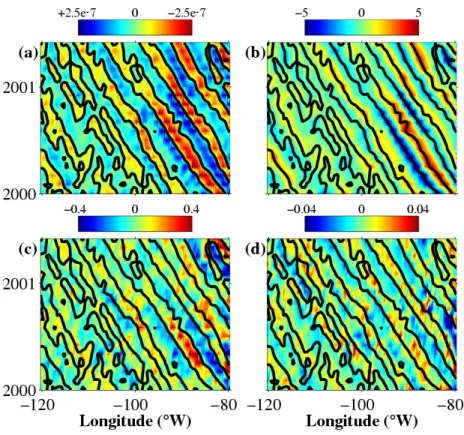
The relationships observed in May 2000 (Fig. 1) can be extended all along RW westward propagations in the 15°S-22°S band (Fig. 2). RWs related anomalies are clearly observed in all diagrams. Again, positive ChlA and SSTA are located in convergence regions. All of this strongly suggests that the vertical motions induced by RWs are not the dominant mechanisms at work to explain the location of ocean-color signals propagating along with RWs.
Figure 2. Longitude-time diagrams of satellite observations in the south Pacific subtropical gyre at 20 °S. (a) convergence, (b) SLAs, (c) SST anomalies, and (d) chlorophyll-a anomalies. Positive (negative) values are represented by red (blue). Black contours of the convergence field are replicated on all panels. For sake of clarity, only the area between 80°W and 120°W, and from January 2000 to June 2001 is represented.
4 If ChlAs are not caused by the usual mechanisms in these RWs systems, it may be that they are not really chlorophyll anomalies. We have then to consider a possible artifact in the determination of chlorophyll from ocean color in the studied region. The ocean color algorithms (14) estimate chlorophyll concentration using the 443 (blue) to 550 nm (green) reflectances ratio (B/G) decreases with increasing chlorophyll concentration. The retrieval of chlorophyll from B/G assumes that the various absorbing and backscattering organic constituents of seawater are in constant proportions. This assumption is generally reasonable, as attested by the extensive use of ocean color data in many studies, but may sometimes lead to biases, even in the open ocean. A bias in SeaWiFS estimates (up to 100 % greater than chlorophyll measured in situ) in the Mediterranean Sea has thus been attributed to non algal particles in excess compared to standard oceanic waters with the same chlorophyll content (15). This bias was observed in low chlorophyll waters such as those investigated in this study. Non algal particles in excess indeed tend to decrease B/G. Likewise, B/G decreases when blue absorbing dissolved colored organic matter is abundant (16). Therefore, it must be kept in mind that B/G, used by all ocean color sensors, also varies with non chlorophyll containing substances. The reported small deviations may thus be nothing but the result of biases in the retrieval of chlorophyll from space. There remains to be explained how these biases are co-located with the convergence/divergence patterns.
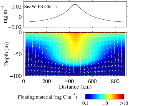
Figure 3. Numerical simulation of the dynamics of floating particles that may generate satellite detected chlorophyll-like anomalies. Lower panel: convergence of floating material (fPOC). Circulation in the vertical plane (adjusted to the observed RW dynamics) concentrates fPOC at the convergence of surface current, where its interaction with light results in lower blue/green reflectance ratio. This is "seen" by SeaWiFS algorithm (upper panel) as chlorophyll
concentration higher than in the divergence areas on both sides from where fPOC is removed. We assume now that low density non-chlorophyllous metabolites and detritus, further mentioned as floating particulate organic carbon (fPOC), are generated by the ecosystem, and accumulate near the sea surface (17). RW induced transport of fPOC tends to remove it from divergences and to accumulate it in convergences where it remains near the surface while
seawater subducts. These substances modify the transfer of light in the sea (18, 19) and should be detected by SeaWiFS as chlorophyll anomalies. To test this hypothesis, we simulate the convergent/divergent vertical circulation across RWs, and the production and advection of fPOC (20) (Fig. 3b). The model transfers fPOC from the upwelling to the subduction areas where it is trapped at the sea surface, generating a strong horizontal gradient (Fig. 3b). Marine reflectances at SeaWiFS wavelengths are then simulated using a radiative transfer model in which only fPOC varies (21). Finally, apparent chlorophyll concentration is computed using the SeaWiFS algorithm (14) (Fig. 3a). In spite of constant chlorophyll concentration in the model, the apparent chlorophyll variability (0.04 mg m-3) caused by fPOC and that affects SeaWiFS detection is coherent with the observations. Model sensitivity tests indicate that fPOC concentration near the surface increases with floatability, and decreases with decay rate. fPOC production, which was set to 1% of primary production in the model, may be given greater values: sediment traps oriented upward and downward have measured an upward flux of particles as high as 2/3 of the downward flux (17). Thus, if production exported to depth is 6% of primary production, a typical value in tropical oligotrophic waters (22), up to 4% of primary production may result in fPOC, leading to an increase four times higher than in our simulation. Presence of gas bubbles, coated with organic film or trapped in fPOC, would also increase the light backscattering coefficient, and thus cause larger bias (23). This simple model, forced by realistic values, provides a framework by which to understand how fPOC can be seen as apparent chlorophyll excess at the RW convergences. However, we need field evidence of particles concentration at the sea surface by this process.
If our hypothesis is valid, then, SeaWiFS estimates would be higher than in situ chlorophyll especially in convergences. Field data to demonstrate such overestimation are scarce. We could however test it using the difference between SeaWiFS chlorophyll estimates and collocated in situ chlorophyll data from twelve cruises from 1999 to 2002 (http://www.lodyc.jussieu.fr/gepco/). Each of these cruises includes 7 to 9 determinations (Chlorophyll a + divinyl chlorophyll a) between 18°S and 25°S on the shipping route from Tahiti to Auckland. Only 20 out of ~100 measurements were co-located with SeaWiFS daily level 3 data (Fig. 4). While these data were collected farther west than 120°W, in an area where Rossby waves energy tends to dissipate (8), they indeed show an inverse relationship (r2 = 0.21, significant at the 95 % confidence level) between local divergence and the difference SeaWiFS minus in situ chlorophyll.
An additional argument is provided by wind data: under strong wind conditions, fPOC should be dispersed in the mixed layer and not be seen from satellite, in the same way as slicks generated by Langmuir circulation cells, rich in floating material (24), are dispersed when wind speed exceeds 6 m s-1 (25). Fields of convergence and ChlAs such as those presented in Fig. 1 are positively correlated. We computed a time series of this correlation from October 1997 to March 2001. It was lowest, around 0.2, in 1998 and until early 1999, during a strong La Niña episode when average wind speed (26) exceeded 6 m s-1. Later, wind speed decreased and correlation improved, around 0.35. Low correlations are also found in austral winter and spring when wind speed increases. Oppositely, high correlations characterize low wind periods, such as May-June 1999, and December 1999-January 2000.
Thus, while direct observations of particles concentration in convergences are still lacking, the obvious effect of average wind speed, together with the higher values of SeaWiFS minus in situ chlorophyll found in convergences, support our hypothesis.
6
Figure 4 : Relationship between divergence of the surface current and the difference SeaWiFS Chl - in situ chlorophyll. In situ chlorophyll were collected during the GeP&CO programme (http://www.lodyc.jussieu.fr/gepco), in the area 15 °S – 25 °S, 150 °W – 170 °W. The difference is computed using daily level 3 SeaWiFS chlorophyll estimates with in situ data. Only collocated data separated by dt (in hour) and dl (in km) such that dt + 0.5 dl is less than 10 are considered. This criterion was adopted to select enough data points (only one GeP&CO measurement was exactly co located with a SeaWiFS estimate). Influence of this arbitrary choice on the final result is small. Divergence is computed using non-filtered weekly altimetry data (7, 10), interpolated at the date and location of the chlorophyll measurements.
There is little doubt that the sea surface is a layer where many substances tend to congregate (17, 24). However, we know very little about this process. Oceanographic cruises usually skip the upper 2 or 3 meters due to practical sampling constraints. It is thus presently not possible to give an exact picture of fPOC. It can consist of flocculated colloids, or detritus, in which bacterial activity has evolved bubbles. The neston is adapted to stay just below the surface and to resist downward water motion. Some phytoplankton species adjust their floatability according to their nutrients content or light requirements. This is the case for some Rhizosolenia sp. diatoms (27) that may make “lines in the sea” in nutrients-rich environments (28); however, this later process is not likely to occur in the oligotrophic South Pacific Subtropical Gyre. Control of floatability by gas bubbles such as in some picoplanktonic cyanobacteria (29) might more likely play a role here. A two step mechanism may also act: after maturation time, accumulation of organic material at the sea surface favors the growth of bacteria, and hence nutrient regeneration (19), and in turn, phytoplankton growth and chlorophyll increase.
Processes that do not need the supply of new nutrients are seldom proposed to explain the biological variability in the oceans. We have shown that the image of a Rossby wave-powered “rototiller” eroding the nutrients-rich deep waters (6) does not apply in the South Pacific Subtropical Gyre. A “hay-rake” (another agricultural machine) that concentrates in restricted
areas the organic material produced uniformly around by the marine ecosystem, provides a better representation of the processes at work. This implies a decoupling of biogenic particles from water circulation, as it is based on substances that float. The JGOFS decade has been devoted to the downward flux of particles. Here, we show that a flux of floating particles can lead to increased concentrations of material in convergence areas, including fronts and subduction zones. This is of interest, first because it may modify ocean color and be detected from satellites, second because it may affect the gas exchange through the air-sea interface, and third because it may be a source of food for fish that live near the surface. Further, as satellite detected sea color is often used to validate biogeochemical models, adding floating material in these models may improve the simulations in places where convergence and fronts occur.
References and Notes
1. L. Legendre, J. Geophys. Res. 103, 2897 (1998)
2. J. R. Christian, M. R. Lewis, D. M. Karl, J. Geophys. Res. 102, 15 667 (1997).
3. D. J., Jr. McGillicuddy et al., Global Biogeochem. Cycles, 17, 10.1029/2002GB001987 (2003). 4. B. M. Uz, J. A. Yoder, V. Osychny, Nature, 409, 597 (2001).
5. P. Cipollini, D. Cromwell, P. G. Challenor, S. Raffaglio, Geophys. Res. Lett., 28, 323 (2001). 6. D. A. Siegel, Nature, 409, 605 (2001).
7. Sea level anomalies from the combined TOPEX/Poseidon and ERS altimeters are produced by the CLS Space Oceanography Division (30). Fields from September 1997 to June 2001 have been interpolated on a 0.25° x 0.25° grid. Several interpolation techniques were applied, giving no relevant differences, and linear interpolation was adopted. Altimeter data were band-pass filtered to extract the signal at observed RW wavelengths and periods (300 km to 5000 km and 3 months to 46 months). The filter, a two-dimensional finite impulse response filter, was applied on longitude-time diagrams (5). Harmonic fit was used to remove the annual cycle of the monthly series, followed by a zonal detrending of the residuals.
8. A. Vega, Y. du Penhoat, B. Dewitte, O. Pizarro, Geophys. Res. Lett., 30, 10.1029/2002GL015886 (2003).
9. J. D. McNeil, H. W. Janasch, T. Dickey, D. McGillicudy, M. Brzezinski, C. M. Sakamoto, J. Geophys. Res., 104 , 15537, 1999.
10. Zonal (u) and meridional (v) currents are computed from SLA as u = - (g/f) ∂(SLA)/∂y and v = (g/f) ∂ (SLA)/∂x where x and y are the zonal and meridional coordinates, g is gravity, f=f0 + βy is the leading part of the variation of the Coriolis parameter, f0 = 4.97 10-5 s-1 is the Coriolis parameter estimated at 20 °S, and β = 2.27 10-11 s-1 m-1 is the meridional derivative of f. Given the continuity equation, and the 1st baroclinic mode assumption, divergence
(convergence) div = ∂u/∂x + ∂v/∂y = -β v/f0 of the horizontal flow is compensated by upwelling (downwelling) at the thermocline depth (31).
8 11. Sea surface temperature from the NASA-NASDA TRMM Microwave Imager (TMI) is
provided by Remote Sensing Systems, interpolated and filtered in the same way as altimetry data.
12. Ocean color data are from the SeaWiFS Global Area Coverage (GAC) level 3 Standard Mapped Image data from NASA-GSFC DAAC (monthly composites), interpolated and filtered in the same way as altimetry data.
13. S. Neuer et al., Geophys. Res. Lett., 29, 10.1029/2002GL015393 (2002). 14. J. E. O'Reilly et al., J. Geophys. Res., 103, 24937 (1998).
15. H. Claustre, et al., Geophys. Res. Lett., 29, 10.1029/2001GL014056 (2002).
16. K. L. Carder, R. G. Steward, G. R. Harvey, P. B. Ortner, Limnol. Oceanogr. 34, 68 (1989). 17. K. L. Smith, P. M. Williams, E. R. M. Druffel, Nature, 337, 724 (1989).
18. D. A. Siegel, A. F. Michaels, Deep-Sea Res. II, 43, 321 (1996). 19. J. J. Cullen, M. R. Lewis, J. Geophys. Res., 100, 13255 (1995).
20. The 2-D (longitude, depth) circulation of the conceptual model is calculated by imposing a stream function giving surface current values peaking to 10 cm s-1 in agreement with the sea-level derived currents. It is limited to the top 100 m, i. e. the average euphotic depth and mixed layer in the south tropical Pacific, and its zonal extension of 900 km represents a typical RW zonal extension. This model simulates the production of fPOC and its accumulation at RW convergences assuming constant biogeochemical conditions in the vertical. Chlorophyll concentration is set to 0.08 mg m-3, and particulate organic carbon (POC), is set to 28 mg m-3, as reported for this area (32). Net primary production decreases exponentially with depth as it is the case for light, amounting to an integrated value of 0.3 g C m-2 d-1, typical of the subtropical gyres. Production of fPOC is set to 1% of net primary production, and this material is given an ascending speed equal to 1 m d-1. One tenth of fPOC in the upper one meter is destroyed each day, simulating its natural decay by
photodegradation or grazing. With such source and sink, the equilibrium for fPOC is 60 mg C m-2 in the water-column. This is a small addition to the system as it represents only 2% of the POC estimated at 150°W, 16°S (32).
21. The Hydrolight (33) simulations were carried out for an infinitely deep ocean with a nearly flat sea surface, and a sun in a black sky, and used standard particulate volume scattering phase function (34), and absorption and scattering coefficients by pure sea water. The scattering coefficient by particles is parameterized as a function of total POC, with total POC=28.0 + fPOC. The wave-length (λ) dependent absorption coefficient by particles is assumed to be the sum of the absorption by phytoplankton, aΦ, and another term, aPOC, representing the contribution of POC in the absorption process. aΦ(λ) is calculated as a function of chlorophyll (35), and aPOC(λ) is equal to aPOC(440) exp(-0.011 (λ – 440)), where the dependency of aPOC(440) on POC is the same as for non algal particles (36).
22. A. K. Aufdenkampe, J. J. McCarthy, M. Rodier, C. Navarette, J. Dunne, J. W. Murray, Global Biogeochem. Cycles, 15, 101 (2001).
23. X. Zhang, M. R. Lewis, B. Johnson, Appl. Opt., 37, 6525 (1998).
24. L. R. Haury, C. L. Fey, E. Shulenberger, Deep-Sea Res. I, 41, 1191 (1994). 25. J. C. Romano, Deep-Sea Res. I, 43, 411 (1996).
26. Weekly 1° x 1° gridded wind fields from the ERS-1/2 scatterometer were provided by CERSAT (IFREMER).
27. T. A. Villareal, S. Woods, J. K. Moore, K. Culver-Rymsza, J. Plankton Res., 18, 1103 (1996). 28. J. A. Yoder, S. G. Ackleson, R. T. Barber, P. Flament, Nature, 371, 689 (1994).
29. B. B. Wallace, and D. P. Hamilton, Limnol. Oceanogr., 44, 273 (1999). 30. N. Ducet, P. Y. Le Traon, G. Reverdin, J. Geophys. Res. 105, 19477 (2000). 31. A. E. Gill, Atmosphere Ocean Dynamics, Acad. Press, New York, 662 p., 1982. 32. H. Claustre et al., J. Geophys. Res. 104, 3401 (1999).
33. C. D. Mobley, “Hydrolight 4.0 User’s Guide”, (Sequoia Scientific, Mercer Island, WA, 1998).
34. T. J. Petzold, “ Volume scattering functions for selected natural waters”, (Tech. Rep. Ref. 72-78, Scripps Institution of Oceanography, San Diego, Calif., 1972).
35. A. Bricaud, M. Babin, A. Morel, H. Claustre, J. Geophys. Res. 100, 13321 (1995).
36. A. Bricaud, A. Morel, M. Babin, K. Allali, H. Claustre, J. Geophys. Res. 103, 31033 (1998). 37. The Hydrolight simulations of marine reflectances at SeaWiFS wavelengths have been done
at Scripps Institution of Oceanography, USCD, by Jacek Piskozub, now at Institute of Oceanology PAS, Sopot, Poland. We acknowledge discussions with J. C. Romano and G. Gorsky. A. Vega benefited from a grant from IRD.