Science Arts & Métiers (SAM)
is an open access repository that collects the work of Arts et Métiers Institute of
Technology researchers and makes it freely available over the web where possible.
This is an author-deposited version published in:
https://sam.ensam.eu
Handle ID: .
http://hdl.handle.net/10985/8300
To cite this version :
Florence DANGLADE, Jean-Philippe PERNOT, Philippe VERON - On the use of Machine
Learning to Defeature CAD Models for Simulation ComputerAided Design and Applications
-Vol. 11, n°3, p.358-368 - 2013
On the use of Machine Learning to Defeature CAD Models for Simulation
Florence Danglade, Jean-Philippe Pernot and Philippe Véron
LSIS Laboratory - CNRS Unit n◦7296, Arts et Métiers ParisTech, Aix-en-Provence, FRANCE
florence.danglade@ensam.eu;jean-philippe.pernot@ensam.eu;philippe.veron@ensam.eu
ABSTRACT
Numerical simulations play more and more important role in product development cycles and are increasingly complex, realistic and varied. CAD models must be adapted to each simulation case to ensure the quality and reliability of the results. The defeaturing is one of the key steps for preparing digital model to a simulation. It requires a great skill and a deep expertise to foresee which features have to be preserved and which features can be simplified. This expertise is often not well developed and strongly depends of the simulation context. In this paper, we propose an approach that uses machine learning techniques to identify rules driving the defeaturing step. The expertise knowledge is supposed to be embedded in a set of configurations that form the basis to develop the processes and find the rules. For this, we propose a method to define the appropriate data models used as inputs and outputs of the learning techniques.
Keywords: CAD model defeaturing, simulation, machine learning, decision making.
1. INTRODUCTION
In the field of artificial intelligence, machine learning techniques [17] aim at identifying complex relation-ships characterizing the mechanisms that generate a set of outputs from a set of empirical inputs, both been considered as inputs data for the underlying algorithms. Once the relationships or rules identified, predictions can be performed on new data. In the field of numerical simulation, the adaptation and idealiza-tion processes of CAD models to prepare simulaidealiza-tion models can be seen as a completion of complex tasks involving high-level expertise and many operations whose parameterization relies on a deep knowledge not often clearly formalized. To address this prob-lem, machine learning techniques can be a good mean to find rules that drive the CAD models preparation processes. Moreover, those techniques can be very helpful to capitalize the knowledge embedded in a set of adaption scenarios.
Depending on the objective of the targeted simula-tion (structural, dynamic/fluid/heat transfer simula-tions, assembly/disassembly procedure evaluations), as well as on the type of method adopted for solv-ing it (Finite Differences, Finite Elements Analysis and so on), there exists a large amount of possible treat-ments to prepare the simulation model from an initial
CAD model (feature removal, part or sub-product removal, shape simplification, size reduction, mesh-ing, meshing adaptation). Figure 1 shows multiple representations a CAD model may have depending on the targeted simulations. These treatments can be applied in different orders and with different tools. Treatment sequences strongly affect the processing time as well as the result accuracy of the simulation solutions.
Among these treatments, the CAD model defeatur-ing is an essential step which aims at removdefeatur-ing irrel-evant features according to a given simulation objec-tive. Indeed, these suppressions are supposed not to affect the simulation results, and they can strongly speed up the overall simulation process. Thus, for a new case study, it is important, not only to find the appropriate defeaturing scenario, but also to be able to identify its impact on the performance of the over-all process. Today, these preparation processes are not well developed. Currently, to select the best treat-ment, expert choices are based on indicators such as the targeted accuracy, cost or preparation time. These indicators must take into account a large num-ber of data relative to the simulation objective, CAD model characteristics and practical industrial con-straints. Thus, the evaluation criteria are difficult to quantify and generalize. Particularly, when selecting
Fig. 1: Multiple representations of a CAD model adapted to different simulation objectives. features (e.g. rounds, chamfers, holes, bumps,
pock-ets, free-form features) to be deleted or preserved, the choice is often empirical and leads, by precaution, to be more precise than necessary (i.e. some features are preserved when they could be removed).
This paper focuses on the way machine learning techniques [10] can be used for understanding how to choose the candidate features for the defeatur-ing steps. Here, the difficulties concern the definition of the right data models given as input and output to the learning techniques. For example, the type of feature, its volume compared to the overall volume or the relative distance between the feature and the applied loads are possible due to relevant variables. Therefore, among these possible variables, it is impor-tant to identify the thresholds that drive engineers during their decision process. The following section present the related state-of-the-art, then the proposed framework is described in section3 and detailed in section4with some results.
2. IMPORTANCE OF THE WORK AND RELATED STATE-OF-THE-ART
Today, it is quite difficult to prepare a simulation model while optimizing the preparation steps that rely on a deep knowledge and strong expertise not always clearly developed and thus hardly automated. Thus, numerous iterations are often required to get an optimal CAD model adapted to a given simula-tion. This contributes to extend product development cycles.
The simplification of CAD models [2,3,8,16] may rely on different mechanisms such as feature simpli-fication [18], feature removal [7], face/volume removal [14], face/volume reconstruction, smoothing, wrap-around [5], etc. They are adapted to the different types of geometric models (e.g. native CAD models, B-Rep models and even meshes [1]) and to various purposes (e.g. visualization, mesh modification). Based on those mechanisms, specific tools have been developed and are constantly evolving. Thus, their functions might no longer be available, or a new version with new functions might make the preparation of certain oper-ations much more efficient or faster. Currently, most of the existing tools are aimed to simplify a geo-metric model for visualization purposes. Unfortu-nately, for physical simulation purposes, these tools do not sufficiently take into account the targeted simulation diversity and the associated industrial
constraints. Moreover, considering the defeaturing step, the choice of the items to be deleted or retained is still a decision that mainly relies on the knowledge and expertise of the engineers.
The experts select the candidates for defeaturing (e.g. rounds, chamfers, holes, bumps, pockets, free-form features) based firstly on the feasibility and accuracy of simulation results for a given objective. However, the experts often don’t know in advance the impact of the defeaturing on the simulation. They select the features for the defeaturing from their com-petence estimating that the impact on the results is negligible and the computation time is faster.
For example, for heat transfer simulation, the expert will decide to delete all rounds. On the same part, for deformation simulation, the expert will decide to delete all rounds away from boundary con-ditions (BC) and to keep the large size rounds close to boundary conditions.
Other requirements are also taken into account such as mesh quality and cost of preparation and simulation (calculations duration, user’s intervention duration, cost of tools . . . ). The additional cost due to the preparation must be compensated by a decrease in the cost of the simulation. Mesh quality and results accuracy must be right without making unnecessarily high quality.
Machine-based Learning tools are widely used in design activities throughout the product life cycle to address optimization problems [11], decision mak-ing problems [6,13], shapes recognition [4,9,13], item recognition and extraction for reuse, recognition from point cloud scans and reverse engineering [2].
Thus, in this paper, we use machine learning to capitalize the expert knowledge and to provide a deci-sion support during the defeaturing steps. First, we will use these tools to estimate numeric variables (e.g. duration and cost of preparation or simulation) or qualitative variables (e.g. features classification depending on their size “small/ medium / large”, rel-ative position to the boundary conditions “feature= BC, feature near BC, feature away from the BC,...”) for which no rules are formalized. Then, from these vari-ables, machine learning tools provide rules to propose candidates for defeaturing.
3. PROPOSED FRAMEWORK
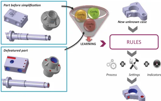
The proposed approach is illustrated on the figure2. The knowledge and expertise are held by experts
Fig. 2: Overview of the proposed approach to defeature CAD models for simulation models preparation.
who will mobilize them to process multiple configu-rations. Following the learning step, the analysis of these numerous configurations will help identifying the rules and thresholds that drive the definition of the processes, of the settings as well as the indicators used to characterize their performance. These rules can be reused in other studies on unknown cases. The so-called “configurations” correspond to sets of CAD models before and after defeaturing, infor-mation characterizing the defeatured CAD models, information describing the preparation processes set-tings of all the treatments and process performance indicators.
To help the engineers make the right decision at each step, one solution would be to store a very large number of simulation configurations, and then compare a new given case within the database. This concept will not take into consideration the evolution of tools and the designers’ requirements. Moreover, this database is constantly evolving and may not con-tain all possible cases. We propose to use the tools of machine learning for proposing defeaturing can-didates for a case study which does not exist in the database.
The framework proposed on figure 3 shows the main steps and data flow. As a summary, the idea is to create an initial database containing known con-figurations (phase 1). According to the learning goal and targets, some data are selected and then put in a learning database. Series of iterative experiments are carried out to identify a learning model and propose ranking rules (phase 2). In this second step, complete-ness and accuracy of data are checked, the learning model repeatability and reliability are analyzed to select the most relevant learning model. Finally, those rules can be applied on new cases (phase 3) that can
also be included into the database to further improve the current rules and thresholds (phase 4). The phases from 1 to 4 are developed subsequently.
4. DETAILS OF THE PROPOSED FRAMEWORK In this section, the proposed approach is detailed. Concrete examples are then provided in section5that comes back on the notions and concepts introduced hereunder.
4.1. Database Construction (Phase 1)
The initial database contains a set of collected infor-mation. Depending on the learning objective, the problem is to identify and select relevant data and to process them in order to create a database for machine learning processing. It contains explanatory variables and also variables to estimate. Divided into two groups “training” and “test”, these variables are used to define rules which estimate the variables from the explanatory one.
4.1.1. Data collection
The initial database must include a significant number of already known configurations and scenarios. The two data sets the input one (CAD model characteris-tics before simplification, designers’ needs and indus-trial constraints), and the output one (CAD model characteristics after simplification, process settings and performance indicators) are then identified.
The CAD model characteristics correspond to information like the type of CAD model (e.g. compo-nent or assembly), the format (e.g. CATIA native, STEP, IGES, tessellated model), the material, the component
Fig. 3: Data flow and framework of the proposed approach.
family (e.g. longitudinal, solid, tubular, thin) and the dimensional quantities (e.g. size, surface area, vol-ume, number of triangles, number of faces). The data related to the CAD models before simplifications are
extracted directly from the initial models or entered by the operator. The data related to the CAD mod-els after simplification are then extracted from the CAD models while being simplified by experts. This
data must be as exhaustive as possible and thus the selection of useful data will be in phase 2 “learning”.
The data related to designer’s needs specify the simulation goal (e.g. stress analysis, displace-ments analysis, fluid transfer, heat transfer, vibra-tion modes), the required level of accuracy on the results, and the aim of the simulation and the bound-ary conditions and loads applied on features, points, edges, surfaces or volumes. Data about industrial con-straints are information like the maximal cost and/or duration for the preparation process and the simu-lation processing, the availability of tools, the level of autonomy of the tools (automated operations, or requiring little user intervention will be preferred).
We will see in the phase 2 “training” that inter-mediate data are necessary to find output data from the input data. This intermediate data refers to stud-ied statistical entities (e.g. characteristics of analyzed features, settings functions) or data clusters (several input data can be grouped into a single intermediate data).
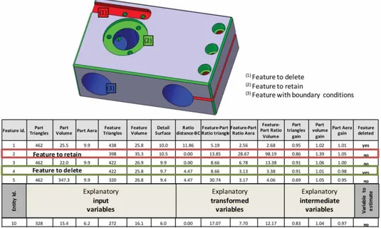
The learning database is a spreadsheet shown on figure4whose rows contain targeted learning entities The columns (except the last one) contain the explana-tory input and intermediate variables, and the last one contain the output variable to estimate. The main objective of this study is to identify these fields and to ensure their completeness. We have to begin choos-ing the aims (variable to estimate in the last column) and the targets of learning (rows). Then, we will select, transform and repair data from initial database in order to create a database for learning.
4.1.2. Definition of learning aims
This step defines what has to be returned to the vari-ables to estimate the last column of the database.
The main learning’s aim is to provide ranking rules in order to be able to identify the features which have to be removed or retained. The output data column, for our aim in this work (defeaturing), contains a qualita-tive data with two possible values “to delete” or “to retain”.
4.1.3. Definition of learning target
The learning targets correspond to studied entities and can either be a feature (feature, set of surface or set of volume extracted from a cad model) or a set of features grouped according to their charac-teristics (“large holes near the boundary conditions”, “small chamfers” “small holes distant from boundary conditions ...).
4.1.4. Selection of input data
The selection, transformation and repair of the input variables determine the accuracy of the results. These steps are the most important of the study. They con-sist in selecting explanatory variables useful for the learning’s aims and to eliminate the variables that may render the analysis false. Among the data set, some are considered as indiscriminate because of the study restriction (material, CAD model type, goal sim-ulation) were removed from the list of explanatory variables. Variables irrelevant, or non-discriminatory for learning aim, or too correlated to each other should be ignored by factor analysis. The explanatory variables selected by the experts are:
• Variables relative to the part before defeatur-ing: surface area, volume, length, width, height, triangles’ number and faces’ number.
• Variables relative to the part after defeatur-ing: surface area, volume, triangles’ number and faces’ number.
• Variables relative to the feature: surface area, volume, length, width, height, triangles’ num-ber, number of similar feature, relationship with other features, relation with boundary condi-tion, distance with boundary condition.
Currently, decision trees themselves detect the variables most discriminating and thus this selection can be done during the family model selection step. A ranking on the full set of variables has identified most significant variables for the main goal: the volume gain, the area gain, the ratio feature/part area, the ratio feature/part volume, the ratio feature/part tri-angles’ number, the distance ratio feature/boundary condition, the feature ratio area/volume, the fea-ture lengths ratio, the feafea-ture compactness and the relationship with other features.
4.1.5. Data repair
Repairing and transforming the variables might be useful to correct final errors due to:
• Size variation of different products: The database must contain CAD model of varying sizes. Thus, the dimensional sizes of CAD mod-els will be replaced by dimensionless ratios whereas the distances are expressed in ratio between the measured distance and the largest distance from the component (e.g. distance between feature and boundary condition/main product dimension); features general charac-teristics are expressed in ratio between tures and component characteristics (e.g. fea-ture’s number of triangles/product’s number of triangles); area, volume and triangles’ num-bers gain are expressed in ratios between area/volume/triangles’ numbers before and after simplification.
• Variation of orders of magnitude: A large vari-ation of the orders of magnitude between two variables influences the final result. Thus, a fac-tor is applied to different variables in order to smooth the orders of magnitude of the vari-ables.
• Irregular values. Irregular values due to an input error, a calculation error, or a poor expert assessment could create an imbalance in analy-sis. They must be detected using statistical tools or through the analysis of the results given by different learning models. These irregular values must be removed (the database may contain a small number of missing values) or replaced by a more realistic value.
• Asymmetric distribution. An analysis of the dis-tribution of the variables will identify a possible
asymmetry (values are then transformed by a function to approximate a normal distribution which will provide best results).
• Qualitative, continuous and discrete data. We have three types of data: qualitative, digital continuous or digital discrete. Some learning models require the transformation of qualita-tive data into discrete data. If some continuous values are not useful (e.g. ratio of the feature’s number of triangles/product’s number of tri-angles), we can simply classify the data into discrete (4-5 classes are sufficient) that will solve the problem of extreme values or missing. The data thus prepared are distributed in two sets: a training set (66%) and a test set (33%) statistically equivalent.
4.2. Learning (Phase 2)
4.2.1. Preliminary model families selection
In this step, we are looking for predictive models which shall meet the following criteria:
• The learning model must be able to classify a qualitative variable;
• The accuracy of the results obtained by the learning model must be within a tolerance imposed by the user. Regarding the main aim, the variable to be estimated is qualitative. Specifically, no features to be retained should be removed; to the reverse a percent error pro-posed by expert is allowed.
• The learning model must take into account the heterogeneity of explanatory variables, which can be qualitative, continuous or discrete. • The learning model shall have good readability
and be robust.
• In the context of this feasibility study we are working with few data (<1000 configurations). Therefore, models which require a large amount of data will be dismissed for a future deploy-ment with many values.
Regarding the results of the qualitative variables for the main aim (feature removal or conservation) or for intermediate aims (family parts or features) selected predictive models are decision trees, regres-sion logistics, neural networks, Bayesian classifier and support vector machine.
4.2.2. Verification of data completeness
Here, previous experiments on training set data can validate the data completeness for the main objective and, all results relating to secondary aims are known. Some learning model like decision tree can iden-tify useful explanatory variables. Tests are restarted by limiting the explanatory variables to those actually
discriminating. A bad and incoherent score for all models shows a lack of explanatory variable.
The need of new variables can then appear, i.e. the necessity to know the studied product family (e.g. thin, tubular, and solid). These new variables will themselves be estimated using machine learning tools. The same approach is carried out to check data completeness necessary for the intermediate results estimation.
4.2.3. Data corrections
Results are analyzed for each explanatory variable and each statistical entity. We can have three cate-gories of errors: acceptable error (the model classifies a feature class as “to retain” instead of “to delete”), unacceptable error (the model classifies a feature class as “to delete” instead of “to retain”), and input error. These input errors are identified by a recurring mistake for all learning, e.g. the models give the right value but the input value given by expert is wrong. Wrong input values are either excluded or replaced by a more realistic value. This phenomenon is illustrated in the next section.
Problems of correlation between the variables can be demonstrated, in this case, several variables are then combined into a single variable (e.g. all variables describing the feature shape can be grouped in an explanatory variable “family feature”).
We obtain at last a reliable basis for determining learning rules.
4.2.4. Learning experiments and evaluation of the most relevant learning model
Experiments on the training sets allowed us to verify our explanatory variables. The accuracy of the results is verified using a simple analysis of the error rates. Less efficient models are rejected. Experiments on test sets will enable us to refine the choice of models and algorithms rules.
Actually, we tested the model repeatability with series of experiments. The choice of learning models is refined by cross validation on both the training and test sets (this is necessary because of the small num-ber of entities we have). The result is compared with experiments on the training set only and then with the test set. A confusion matrix is used to measure the rate of misclassification, indicating the rate of fea-tures well classified, the rate of feafea-tures which must be retained and are removed (unacceptable error) and the rate of features which must be removed and are retained (acceptable error if preparation or simulation are achievable and their performances are decreased in a moderate proportion). The performance mod-els and its robustness are validated with a Receiver Operating Characteristic curve.
At the end of this step the best model is selected. In case of bad results, we repeat all the steps of Phase 2.
4.3. Use of Rules on Unknown Data (Phase 3) Input data related to the new configurations are included in the initial database. Intermediate vari-ables are first estimated with algorithms defined with learning machine tools in phase 2. Then, intermediate variables are included in the database.
4.4. Consolidation of the Rules (Phase 4)
The results obtained from the unknown data can be integrated in the initial database, the latter is thus enriched. New algorithms are then proposed by replaying the approach proposed in phase 2. Thus, a new more complete and more efficient model is identified. This iteration process allows a continual improvement of the knowledge learnt to produce a more and more reliable decision making tool for engineers.
5. ACHIEVEMENTS AND VALIDATION OF THE RESULTS
Among all the simulation objectives, this paper focuses on heat transfer and stress analyses. As depicted on figure 5, 20 parts with about 200 fea-tures were treated. Each test and training learning database contains 100 cases. To implement the pro-posed framework (fig.3), the Weka platform [19] has been plugged to a VBA macro developed within CATIA V5. The output data consist in a list of features to be removed.
In the proposed approach, the evaluation criteria of the learning model are:
• percentage of correctly classified instances: results are given in table1for two experiments; • number of unacceptable results given by the confusion matrix (fig. 7) due to instances clas-sified in Yes instead of No (column “NY” in table 1) or instances classified in No instead of Yes that may decreased indicator performance of preparation (column “IP” in table1);
• results repeatability (table 1 shows results for two experiments with training data set and test data set);
• the shape of the ROC (Receiver Operating Char-acteristic) curve that should be as far as possible from the midline for which results are those obtained by random (fig.7).
From these experimentations, it is clear that the models giving the best results are neural net-works (multilayer perception), decision tree (J48) and support vector machine (SMO). Only the results obtained with these models are given here. Series of experiments were carried out with different learn-ing database. At first, we have experimented all ini-tial databases as explanatory variables. Table 1 and
Fig. 5: Parts studied before simplification.
curves ROC (fig. 7) show that whatever the learn-ing models, the results obtained with the original untransformed data are similar to those that could be obtained by random. For repeatability and robustness criteria, the most relevant learning model is neural network model with 91% of correct values with the test set database. Decision tree model is not excluded because we know that the result will be better with more learning cases (more than 1000 cases instead of 200 here).
Variables ranking selection (detailed list in 3.1) and ratio transformation (3.1) increase the results. The correction of variables concerns the unification of the orders of magnitude for the selected data. Analysis of extreme values has identified irregular values (round considered as a unique large feature) that have been modified (divided into several rounds). Repair data can especially improve the repeatability of the results and gives a better ROC curve.
The explanatory variables feature ratio area/ volume, feature lengths ratio, and feature compact-ness have been grouped in a unique group: fea-ture family. The explanatory variables giving best results are the volume gain, the area gain, the ratio feature/part volume, the ratio feature/part triangles’
number, the feature family and the distance ratio feature/boundary condition.
The examples of figure 6 show acceptable, unac-ceptable and input error as defined in section 3.1. Concerning Part #1, a feature that should be removed has been preserved. This error is unacceptable since the preparation performance is low (simula-tion impossible or very long due to a small mesh). This shows that since the completeness of variables is not satisfied, two solutions are possible, and give the same good result. The first consist in adding a new family feature “thin pocket”, the second consist in adding a new explanatory variable “ratio between the smallest and the largest feature dimension”. Con-cerning part #2, a feature that should be preserved has been removed. The learning model (here the deci-sion tree) cannot be retained. Concerning part #3, all learning model give the same result that is differ-ent from the expert proposition. An analyze shows that the right result is the one proposed by the learn-ing model. Thus, the input data is modified in initial database.
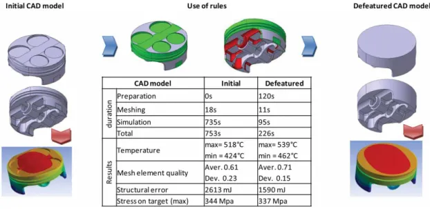
Figure 8 gives results obtained while using the rules on a new unknown case for a heat transfer and stress analysis simulation. 19 features were analyzed, the retained features are essentially thin pockets and
% of correctly Unacceptable classified instances errors
Cross validation Explanatory Learning model
tests variables = training set test set NY IP acceptability
Neural networks Initial data 76.2 50.8 15 12 No
Ranking selected+ ratio trans-formation variables
98.3 64.4 1 1 No
Repaired variables 96 68.4 1 1 No
Grouping variables 99.2 91.2 0 1 Acceptable
support vector machine
Initial data 57.6 47.5 17 13 No
Ranking selected+ ratio trans-formation variables
71.2 56 8 2 No
Repaired variables 66.7 61.4 9 1 No
Grouping variables 68.4 54.3 2 1 No
Decision tree Initial data 61 51 14 9 No
Ranking selected + ratio trans-formation variables
94.9 67.8 1 1 No
Repaired variables 84.2 70.2 2 1 No
Grouping variables 93.5 87.7 1 0 Acceptable
Fig. 6: Estimations examples.
Fig. 7: ROC curve and confusion matrix for test set data.
rounds near the boundary conditions. The accuracy of the results is checked by carrying out a simulation. We note that the quality of the mesh was improved. The simulation duration is reduced by 70% and the error on the temperature values and stress on target simulation is only about 8%. These new values can be used to estimate the overall performance of the CAD model treatment process for simulation.
6. CONCLUSION
In this paper, the way machine learning can be used to learn how to adapt CAD models for simulation mod-els preparation is investigated for a particular step of defeaturing (identification of feature to delete or to retain). A dedicated framework has been set up. It combines several models and tools used to sup-port the extraction of data from initial and simplified
Fig. 8: Use of rules example.
CAD models, the inputs from the experts, as well as the learning mechanisms properly saying. The results are promising and prove that the machine learning techniques can be a good mean to capitalize the knowledge embedded in empirical processes like the defeaturing steps. Actually, from a database whose variables are multiple and heterogeneous, machine learning tools have provided evolving rules unless they are formalized at the beginning. Future work should take into account some points that have not been developed in this feasibility study:
• Sequencing of functions (tools and order of defeaturing) and processing (defeaturing before/after meshing, symmetry use...);
• Hierarchical relationships between the lines of the spreadsheet (the decision on a feature may depend on the decision of another feature); • Several experts for the validation of simplified
models.
The study was limited to analysis stress and heat transfer simulations for single parts, it may be extended to other targets and other types of CAD models.
In the future, such a framework should be extended to support other model preparation steps (e.g. meshing, simplification) as well as the global preparation process (tools selection and sequencing, estimation of cost preparation and simulation). At the end, the proposed approach and tools should reduce significantly the number and duration of design itera-tions, thus improving the product development cycles and increase the reliability of the design processes.
REFERENCES
[1] Gao, S.; Zhao, W.; Lin, H.; Yang, F.; Chen, X.: Feature suppression based CAD mesh model
simplification, Computer Aided Design, 42(12), 2010, 1178–1188.
[2] Gujarathi, G.P.; Ma, Y.-S.: Parametric CAD/CAE integration using a common data model, Jour-nal of Manufacturing Systems, 30(3), 2011, 118–132.
[3] Hamri, O.; Léon, J.-C.; Giannini F.; Falcidieno, B.: Software environment for CAD/CAE integra-tion, Advances in Engineering Software, 41(10– 11), 2010, 1211–1222.
[4] Jayanti, S.; Kalyanaraman, Y.; Ramani, K.: Shape-based clustering for 3D CAD objects: A comparative study of effectiveness, Computer Aided Design, 41(12), 2009, 999-1007.
[5] Koo, S.; Lee, K.: Wrap-around operation to make multi-resolution model of part and assem-bly, Computers & Graphics, 26, 2002, 687– 700.
[6] La Rocca, G.: Knowledge based engineer-ing: Between AI and CAD. Review of a lan-guage based technology to support engineer-ing design, Advanced Engineerengineer-ing Informatics, 26(2), 2012, 159–179, doi:10.1016/j.aei.2012. 02.002.
[7] Lee, S. H.: A CAD-CAE integration approach using feature-based resolution and multi-abstraction modeling techniques, Computer Aided Design, 37(9), 2005, 941–955.
[8] Li, C.; Fan, S.; Shi, M.: Preparation of CAD Model for Finite Element Analysis. International Con-ference on Computer, Mechatronics, Control and Electronic Engineering (CMCE), 2010. [9] Ma L.; Huang Z.; Wang Y.: Automatic discovery
of common design structures in CAD mod-els, Computers and Graphics, 34 (5), 2010, 545–555.
[10] Mitchell, T.: Machine Learning, McGraw Hill, 1997
[11] Renner, G.: Genetic algorithms in computer aided design, Computer-Aided Design and Applications, 1,(1–4), 2004, 691–700.
[12] Shi, B.-Q.; Liang, J.; Liu, Q.: Adaptive simplifica-tion of point cloud using k-means clustering, Computer Aided Design, 2011, 43 (8), 910–922. [13] Chandrasegaran, S.K.; Ramani, K.; Sriram, R. D.; Horváth, I.; Bernard, A.; Harik, R. F.; Gao, W.: The evolution, challenges, and future of knowl-edge representation in product design systems, Computer-Aided Design, 45(2), 2013, 204–228. [14] Sun, R.; Gao, S.; Zhao, W.: An approach to B-rep model simplification based on region sup-pression, Computers & Graphics, 34(5), 2010, 556–564.
[15] Sunil, V.B.; Agarwal, R.; Pande, S.S.: An approach to recognize interacting features
from B-Rep CAD models of prismatic machined parts using a hybrid (graph and rule based) technique, Computers in Industry, 61(7), 686– 701, 2010.
[16] Thakur, A.; Banerjee, A.G.; Gupta, S.K.: A survey of CAD model simplification tech-niques for physics-based simulation applica-tions, Computer Aided Design, 41(2), 65–80.
[17] Wernick, Y.; Brankov, Y.; Strother: Machine Learning in Medical Imaging, IEEE Signal Pro-cessing Magazine, 27(4), July 2010, 25–38 [18] Zhu, H.; Menq, C. H.: B-Rep Model
Simplifica-tion by Automatic fillet/round Suppressing for Efficient Automatic Feature Recognition. Com-puter Aided Design, 34(2), 2002.