Simulation of the Injection Stretch Blow Molding Process: An Anisotropic Visco-Hyperelastic Model for Polyethylene Terephthalate Behavior

Science Arts & Métiers (SAM)

is an open access repository that collects the work of Arts et Métiers Institute of Technology researchers and makes it freely available over the web where possible.

This is an author-deposited version published in: https://sam.ensam.eu

Handle ID: .http://hdl.handle.net/10985/18578

To cite this version :

Yunmei LUO, Luc CHEVALIER, Eric MONTEIRO, Shiyong YAN, Gary H. MENARY - Simulation of the Injection Stretch Blow Molding Process: An Anisotropic Visco-Hyperelastic Model for Polyethylene Terephthalate Behavior - Polymer Engineering and Science - Vol. 60, n°4, p.823-831 - 2020

Any correspondence concerning this service should be sent to the repository Administrator : archiveouverte@ensam.eu

Simulation of the Injection Stretch Blow Moulding Process: an

Anisotropic Visco-hyperelastic Model for PET Behavior

Yun-Mei Luo, Luc Chevalier*, Eric Monteiro, Shiyong Yan, Gary Menary

Introduction

The sustainable use of plastics has become a global issue with all major brand owners committed to reducing the use of plastic in packaging through optimized design or recycling initiatives. An area receiving major attention is the use of PET bottles which are currently manufactured at a rate of one million per minute by a process known as Injection Stretch Blow Moulding (ISBM). ISBM begins with injection molding of a test tube like specimen known as a preform that is subsequently re-heated above its glass transition temperature and formed into a mold by a combination of axial stretching by a stretch rod and radial stretching by internal air pressure. The main challenge for manufacturers is to produce containers with as little material as possible but still meet in-service performance requirements such as top load and burst resistance. However the industry still relies a lot on empirical knowledge and trial and error and it recognizes the need to move away from this approach though the use of manufacturing process simulation. The key component of a the process simulation is the constitutive material model to accurately capture the nonlinear viscoelastic behavior of PET over the wide temperature, strain rates and modes of deformation experienced in stretch blow molding.

An accurate model of PET for stretch blow molding must be characterized at temperatures and strain rates typically seen in the process. Nixon et al [1] demonstrated through free blowing preforms whilst monitored via high speed video that the strain rate has an average of 40s-1_{[1] whilst it is well recognized in the industry the}

temperature range of interest is between 90°C and 120°C i.e. just above the glass transition temperature but just below the cold crystallization temperature.

Over the past 30 years there have been numerous attempts to develop models of the non linear viscoelastic behavior of PET for ISBM. Initially researchers ignored the viscous effects and used hyperelastic models (Marckmann et al. [2]). Billon et al [3,4] recognizing the need to include viscous effects and altered the hyperelastic model by making some of the parameters dependent on strain rate however the model proved to be unstable when implemented in forming simulations. Previous work from Chevalier et al [5] based on biaxial experimental data in the strain rate range 0.02 to 2 s-1 _clearly

demonstrated the need to capture the viscous effects and based on this data a new model known as the G’Sell-Jonas was developed which took into account the effect of strain rate and the typical strain hardening behavior observed in PET. This viscoplastic model

was subsequently used by Schmidt et al [6] to demonstrate the potential of combining simulations of stretch blow molding and IR heating to determine the optimum process settings to manufacture a container with a desired thickness profile. The model was further developed by Cosson [7] through the implementation of anisotropy. Whilst this improved model was also able to relate the constitutive behavior with microstructure due to its viscoplastic nature it was still unable to match data produced in experiments performed by Chevalier and Marco [8].

Other approaches to modelling PET in ISBM is the use of viscoelastic models [9,10]. One example includes the work by Schmidt [9] who used a Maxwell like model, however accurate results for predicting the preform shape evolution and strain hardening behaviour were not achievable. It was clear that a combination of viscoelastic and hyperplastic effects were required to capture the behavior of PET. This was recognized by both Boyce et al [11] and Buckley et al [12] who both developed models of PET through the parallel combination of hyperleastic models and viscous models. The model developed by Buckley et al known as the Glass Rubber model was initially developed for the study of hot drawing of PET in industrial film drawing. Menary et al

[13]evaluated the model for its ability to capture the behavior of PET in stretch blow molding and benchmarked it against the performance of a hyperleastic model and a creep law in an ISBM simulation. It was demonstrated that the Glass Rubber model was able to accurately predict the final wall thickness of a PET bottle.

Inspired from Figiel and Buckley's work [14], Chevalier et al. [15-17] have recently proposed a nonlinear incompressible visco-hyperelastic model to represent the complex constitutive behaviour of PET. Experimental uniaxial and biaxial tests performed on PET were carried out by Menary et al. [18] in Queen’s University of Belfast. These tension tests were managed with various tension speeds (strain rate from 1s-1 to 32s

-1_{),.The nonlinear forms of elastic and viscous characteristics were proposed. However,}

the isotropic version of the model that we proposed [15-17] did not reproduce the shape evolution of the perform during blowing: and thus some improvements are needed to fit biaxial tests and free blowing experiments.

In the first section, based on a previous isotropic version of a visco-hyperelastic model build to represent the behavior of PET near the glass transition temperature, we propose an anisotropic version. The theoretical basements of this upgraded anisotropic version are presented. First, an energy function W models the elastic part with the isotropic contribution Wiso and anisotropic one Wani. The isotropic part Wiso depends on

the classical invariants and the anisotropic part Wani depends on the new invariants that

are associated to the anisotropic material behavior. The stress tensor is obtained from derivation of this energy function W and depends on structural tensor Ai built from the

direction of anisotropy. The viscous part is built using a 4th order tensor to represent the classical orthotropic formulation.

The second section is devoted to the identification procedure to make the model fit with experimental data. This anisotropic version of the visco-hyperelastic model needs both equi-biaxial and constant width to provide an accurate identification. These tests were managed at Queen’s University Belfast. A singularity problem appears for the numerical simulation due to asymptotic values for the h function that represents the strain hardening effect in the viscous part. The h function is modified in order to solve this singularity.

Finally, in the third section, thanks to this identification, we can simulate free blowing of PET preform that is close to the industrial stretch blow molding process. We use the software ABAQUS/Explicit for the simulations and our model is implemented via a user-interface VUMAT. Free blowing simulations taking into account the anisotropy, are performed and are successfully compared to the experimental results.

I. An anisotropic visco-hyperelastic model for PET under ISBM condition

An isotropic version of the nonlinear incompressible visco-hyperelastic model has been presented and identified in the author’s previous papers [15-17]. This model reproduces nicely the equi-biaxial elongation results obtained from experimental tests performed at QUB [18] using strain, strain rate and temperature conditions near ISBM conditions, but this isotropic version did not reproduce accurately the shape evolution of the preform during blowing. Using this version of the model, when the strain reaches the “strain hardening” region in the hoop direction, the material cannot be stretched anymore and this limits the evolution in longitudinal direction. In order to correct this drawback during the free blowing simulation, one needs to introduce anisotropy in both the viscous and elastic parts of the model. This will allow to reproduce accurately the constant width test and will provide accurate simulation of the free blowing of preform. The Cauchy stress tensor  is developed as a Maxwell like equation with two expressions whether one considers the elastic or the viscous part:

2 2 e e v v p I G p I D     = − +   = − +  (1)

where is an Eulerian strain tensor: e _e =

(

B_e−I

)

2 1

 , Dv is the viscous strain rate

tensor, pe and pv are hydrostatic pressures associated with incompressibility

conditions. Be is the elastic part of the left Cauchy deformation tensor. In a previous

isotropic version, G and  were scalar shear modulus and viscosity. Both characteristics were a function of elastic strain components for G and of viscous strain and strain rate for . In the following, we present the anisotropic form of these two parts. First, let’s focus on the elastic part.

I.1 Elastic part visco-hyperelastic model

The free energy function W is defined as a function of two series of invariants: the principal invariants of the elastic left Cauchy Green tensor and also more invariants defined in Spencer [19,20]. The first series is associated to the isotropic material behavior and can be written as:

( )

Be I



tr

( ) ( )

Be trBe



I

( )

Be tr I , det 2 1 , 2 2 ₃ 2 1= = − = (2)

The second series are the invariants associated to the anisotropic behavior:

4 1 1 6 2 2 8 3 3 2 2 2 5 1 1 7 2 2 9 3 3 , , , , , e e e e e e I n B n I n B n I n B n I n B n I n B n I n B n =   =   =   =   =   =   (3) 1

n ,n₂ et n₃ are the privileged directions of the orthotropic behavior of the PET

material. We introduce three second order structural tensors Ai. They are obtained

from the preferred directions [21]:

1 1 1, 2 2 2, 3 3 3

A = n n A =n n A =n n (4)

These structural tensors have to be invariant under the rotation tensor Q out of the symmetry group , so they have to satisfy the condition [21]:

T

i i

Due to the representation theorem, the strain energy W can be rewritten as both an isotropic part and an anisotropic part:

(

B ,A1,A2,A3

)

W

(

I1,I2

)

W

(

I4,I5,I6,I7,I8,I9

)

W _e = _iso + _ani (6)

where Wiso and Wani are isotropic convex functions of their arguments.

We make the assumption that displacements are big enough to neglect the volume variation so : I3=1. The important strain hardening effect that appears during uniaxial

or biaxial tension tests needs to be represented by both the hyperelastic part and the viscous part using exponential functions. For the elastic part, Hart-Smith appears to be a good candidate to characterize the free energy function. Consequently, Wiso is only a

function of I1 and the total energy function can be written as the following form:

(

)

1 2

(

4 2 6 2

)

1 2 2 3 1 1 1 2 3 1 ₀ 2 _{0 0} , , , I X I X I X W B A A A =G



− e dX+G



− e dX+



− e dX (7) Cauchy stress tensor is obtained from the strain energy by derivation [22]:

(

)

(

)

(

)

(

)

2 ,1 1 ,2 ,2 4 ,4 1 4 ,5 1 1 1 1 6 ,6 2 6 ,7 2 2 2 2 8 ,8 3 8 ,9 3 3 3 3 2 2 2 2 2 2 2 2 2 e e e e e e e e e e W p I W I W B W B B I W A I W n B n n B n I W A I W n B n n B n I W A I W n B n n B n  =  = − + + −  + +  +  + +  +  + +  +  (8)

where W stands for the partial derivative _,i W Ii. Considering the chosen energy

function W (Eq.7), the elastic stress yields to:

( )2 ( )2 ( )2 2 6 1 1 3 2 4 1 1 1 4 2 1 6 2 2 2 I 2 I 2 I pI G e B I G e A I G e A   −  −  − = − + + + (9)

where G1, G2,  and  are parameters in the elastic part of the Visco-hyperelastic

model.

I.2 Viscous part visco-hyperelastic model

v

D 

 2 = that also writes:

                    =               12 22 11 44 22 12 12 11 12 22 11 2 0 0 0 0 2 2 _v v v D D D         (10)

We choose specific hi functions [15] for each orthotropic direction (i=1 the hoop

direction and i=2 longitudinal direction)

( )

( )

( )

(

)

( )

( )

( )

( )

( ) ( )

11 0 1 12 0 1 2 22 0 2 44 0 max v v v v v η η T h f d η η T h ,h f d η η T h f d η η T h ε f d  ₌   ₌   =    = 

(

)

(

)

(

)

(

)

( )

(

(

)

)

                     + +          − − =         + +          − − =         + +          − − = 3 2 2 1 3 2 2 2 2 1 2 2 3 1 2 2 1 1 1 1 exp exp 1 exp exp 1 exp exp 1                   v vref v v v v vref v v v vref v v ε ε ε K ε h K h K h (11) with:

( )

(

)

(

)

1 1 1 v m a _a v ref f d d d  − = + ,

( )

2 2 3 v v d = tr D (12)

where , m, a are the classical parameters of Carreau’s law f d

( )

_v and d_ref are arbitrary reference strain rates that can be taken equal to 1s-1 for sake of simplicity. d_v

is the equivalent viscous strain rate and  is the equivalent viscous strain_v . The chosen expressions for hi functions assure to give the same model as the isotropic one when

can be identified from biaxial elongation tests using the previous procedure presented in [15-17]. Under the assumption of additivity of the elastic and viscous strain rates, assumption of the pure elastic spin rate and the choice of the Oldroyd equation for tensor Be , the constitutive equation can be obtained.

Therefore, equation 9 in plane stress case for the deviatoric part of the stress can be written as: ( )2 ( )2 ( )2 2 6 1 1 3 2 4 1 1 1 4 2 1 6 2 2 2D_v 2G e I B_e 2I G e I A 2I G e I A   _{ −}   −  − = + + (13) That implies: 22 12 2 2 11 22 12 11 22 12 11 11 12 22 22 2 2 22 11 22 12 11 22 12 12 ₁₂ 44 0 0 1 0 0 v v v d D D d D _d                   −   _{− −}        _{ }  −   _{ =  }     _{− −  }    _{  }   _{  }     (14) where           12 22 11 ~ ~ ~ d d d

is the column form of the tensors sum

( )2 ( )2 ( )2 2 6 1 1 3 2 4 1 1 1 4 2 1 6 2 2 2G e I B_e 2I G e I A 2I G e I A   _{ −}   − ₊  − ₊

appearing in the right side of equation 13. In the following sections, equation 13 can be used to simulate the tension test and the ISBM process.

II. Identification procedure of the model from equal-biaxial and constant width

tensile tests

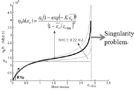
The authors have previously used a specific h function to model the strain hardening effect during the viscous part of the model (see [15] for details). From an arbitrary choice for the hyperelastic part and for the contribution of the strain rate in the viscous part, one can extract from experimental data, the contribution of the elongational strain in the viscous part. The shape of the obtained curves highlights an ultimate viscous

strain but during the numerical simulations using this model, the limit value can be reached and passed: numerical problems arise. More precisely, the singularity problem appears during the ISBM process simulation when the viscous strain is higher than the parameter vlim (Figure 1). Therefore, a purely exponential function is chosen instead of

the original h function presented in previous publications.

(

)

(

)

(

)

(

)

                 + +          − − =         + +          − − = 3 2 2 2 2 1 2 2 3 1 2 2 1 1 1 1 exp exp 1 exp exp 1               v vref v v v vref v v K h K h (15)

The identification process is based on minimizing the square difference between the model and the experimental values of both equi-biaxial and constant width tests. These two problems can be solved quasi-analytically: totally for the equi biaxial test and with a numerical resolution for the constant width. This identification leads to the identified values shown in Table 1. The mean difference between model and experiment highlighted on curves shown Figure 2 is 12.8% for constant width in the elongation direction and 6.2% in the constrained direction. For the equi-biaxial test, the mean difference is 6.3%.

Considering the complexity of the PET behavior and the small number (12) of numerical parameters to be identified in our model, this agreement is good and leads to accurate results.

An analysis of the sensitivity of the model to the parameters value is managed using a partial differentiation technique. In this case, the mean absolute error  depends on each parameter i and can be calculated from equation 16. Each parameter is increased

independently by a value of 10%, the sensitivity coefficient di, can be calculated which

is the difference between the new mean error new and the error with standard

parameters ref. Table 2 lists the sensitivity coefficient di of each parameter in our

model. The parameter m is clearly the most sensitive parameter. The 4 parameters used in the elastic part of the model have less influence.

( )

exp exp exp exp num num CW EB EB CW i EB CW         − − = + (16)

III. Stretching and blowing simulation of a PET preform

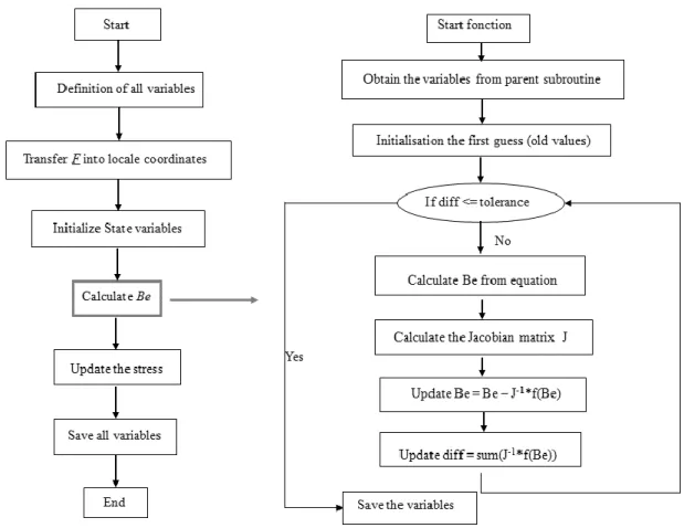
The software ABAQUS / Explicit is used so that geometry definition and meshing operations remains easy. We implement our VHE model via a user interface VUMAT a classical Newton Raphson iterative procedure is used to solve this strongly non linear problem. Figure 3 illustrates the structure of the implementation into the ABAQUS software. One can compute the elastic Cauchy Green tensor Be from equation 14.

III.1 Benefit of the anisotropic model for the free blowing simulation of a PET preform

In order to evaluate the predicting performance of the model, we focus on the simulation of a preform stretched by an internal rod and blown with air at a specific flow rate that generates internal pressure. Using the finite element approach, we will be able to compare the shape and the internal pressure evolution obtained by simulation with experimental data. The preform geometry and the longitudinal stretch rod are meshed by shell elements in ABAQUS. In order to reduce the computing time, we took into account the axi-symmetry of the process and that choice reduces the number of degrees of freedom. The air mass flow injected into the preform / bottle is modelled by an exchange of fluid between components (fluid structure interaction implanted in ABAQUS). This air mass flow modelling has already been described in detail in [1,23,24].

Nevertheless, CPU time for one complete free blow simulation using a 2.66GHz Pentium4 processor is about six hours.

The previous free blow [25] and stretch blow simulation results obtained with the isotropic version of the visco-hyper-elastic model failed to represent the real ratio between the length and radius of final bottles. One explanation is that the isotropic model leads to very high viscosity value once the elements are stretched along one direction (here, the hoop direction). Consequently, the elongation in the longitudinal direction is more difficult.

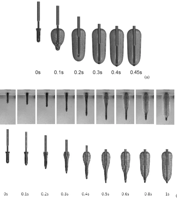
Figure 4 shows the evolution of the bottle shape. One can see that anisotropic version of the model gives a shape evolution that is in good agreement in comparison with the real blown bottle. A free blowing machine developed at Queen’s University [1] made possible the experimental measurements. During the test, the stretch rod velocity, the air flow rate, the maximum blowing pressure within the preform cavity are imposed and the preform stretching force and the pressure evolution vs time are measured. The

details of experimental set up and the data acquisition system were previously described in [26-28]. During a SBM process, the hot preform is transformed into a bottle mainly due to the pressure exerted on the inside walls of the preform by the compressed air. The work of Menary et al. [26] demonstrated that the pressure that builds inside the preform is not a cause but an effect that depends on the amount of air filling the preform and the rate of expansion of the preform. By using the mass flow approach in the simulation, they showed that the preform shape evolution prediction was better than the direct experimental pressure application. Salomeia [27] used an air mass flow model which was described as a function of pressure difference. The mass flow rate is controlled by both the preblow pressure adjuster and the flow limiter. The preblow pressure is 8bar and the mass flow rate has two levels controlled by the flow index (two for low or six for high). The average value of mass flow rate at the higher level is 33.96 ±0.863 g/s, almost four times larger than that of the lower level (8.88±0.195 g/s).

Figure 5 shows the evolution of pressure coming from simulation (discontinuous line) and from experimental results (dots that makes a quasi-continuous line). Considering the complexity of the PET behavior and the small number (12) of numerical parameters of our model, and considering that parameter identification is obtained from an idealized biaxially stretched plane specimen, one can conclude that there is a good agreement between this axi-symmetric simulation and free blowing experiment. Consequently, one can have faith in the model and consider other cases for predicting effects on thickness distribution for example.

III.2 Model validation from numerical/experimental comparison of a stretching and blowing simulation of a PET preform

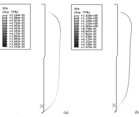
Moreover, two stretch blow simulations have been performed. Figure 6a shows a ‘free blowing’ like simulation: because of the high air flow rate, the material elongation in the longitudinal direction of the preform goes faster than the stretch rod. No contact occurs between the preform and the stretch rod during this specific blowing. The experimental measurements for this ‘free blowing like’ simulation is shown in Fig. 4a. Figure 6b shows another simulation with a lower air flow rate, in this case the material longitudinal elongation is slow. The preform is stretched by the rod at first and then in the hoop direction during blowing. This simulation is also compared with the experimental measurements. The stretch rod velocity for each case is given in Figure 7a. Figure 7b shows for each case the air mass flow rate as a function of pressure difference (dP).

Figure 8 shows the distribution of the thickness of the two stretch blowing cases. In the free blowing like simulation Fig. 8a, the mean value of the thickness is about 0.45mm. The aspect ratio (ie. length over radius) is lower than for the second case. Consequently, for the same global length, the thickness will be higher in the second case.

In the stretch blowing simulation case (right side of the figure), the mean thickness is about 0.5mm and the distribution is more homogenous. In both cases, one can see that the thickness is higher in the zone near the neck of the bottle than elsewhere.

Conclusions

We developed an orthotropic visco-hyperelastic model adapted to the severe strain-rates and temperatures conditions of the stretch-blow molding process. An orthotropic formalism is used for both elastic and viscous parts and the complex form of the model is presented.

The identification procedure has been achieved using data provided by equi-biaxial and constant width elongation tests managed at QUB at different speeds and temperatures. The best parameters values identified for the model enables to reproduce the experimental results with about 10% difference.

We implemented the orthotropic visco-hyper-elastic model in ABAQUS software and we simulate free blowing of PET perform. The comparison with a real free blowing test validates the anisotropic version of the visco-hyperelastic model for PET near Tg.

As a complement, the influence of the air flow rate on the shape evolution and thickness distribution has been managed and high air flow rate leads to larger radius and lower thickness.

References

[1] J. Nixon, G. Menary, S. Yan. International Journal of Material Forming. 10, 5, p. 793-809, (2017).

[2] G. Marckmann, E. Verron, B. Peseux, Polymer Eng Sci., 41(3), 426–439 (2001). [3] E. Gorlier, J.F. Agassant, J.M. Haudin, N. Billon, Plast Rubber Compos Process Appl., 30(2), 48–55 (2001) .

[4] E. Gorlier, J.M. Haudin, J.F. Agassant, J.L., Lepage, G. Perez, D. Darras, N. Billon, The 14th International ESAFORM Conference on Material Forming, Liège, 345-348 (2001).

[5] L. Chevalier, Y. Marco, Int. J. Mech. Mater., 39(6), 596–609, (2006).

[6] M. Bordival, F.M. Schmidt, Y. Le Maoult, V. Velay, Pol. Eng. Sci., 49(4):783–793 (2009).

[7] B. Cosson, L. Chevalier, J. Yvonnet, Int. Polymer Process, 24(3), 223–233 (2009). [8]. L. Chevalier, Y. Marco, G. Regnier, Mec. Ind., 2, 229–248 (2001).

[9] F.M. Schmidt, J.F. Agassant, M. Bellet, L. Desoutter, Journal of Non-Newtonian Fluid Mechanics, 64 (1), 19-42 (1996).

[10] G. Barakos, E. Mitsoulis, J. Non-Newt. Fluid Mech., 58, 315-329 (1995).

[11] M. Boyce, S. Socrate, P.G. Llana, Polymer 41 (6): 2183-2201 (200)[11] C.P. Buckley, D.C. Jones, Polymer, 36, 3301-3312 (1995).

[12] C.P. Buckley, D.C. Jones, and D.P. Jones, Polymer, 37, 2403 -2414 (1996). [13] G.H. Menary, C.G. Armstrong, R.J. Crawford, and J.P. McEvoy, Rubber and Composites Processing and Applications, 29, 360-370 (2000).

[14] L. Figiel, C.P. Buckley, International Journal of Non-linear Mechanics, 44, 389-395 (2009).

[15] Y.M. Luo, L. Chevalier, E. Monteiro, The 14th International ESAFORM Conference on Material Forming, Queen’s University , Belfast, Irlande du Nord, April 27-29, (2011).

[16] L. Chevalier, Y.M. Luo, E. Monteiro, G. Menary, Mechanics of Material, 52, 103-116, (2012).

[17] Y.M. Luo, L. Chevalier, F. Utheza, E. Monteiro. Polymer Engineering &Science, 53(12), 2683–2695, (2013).

[18] G.H. Menary, C.W. Tan, E.M.A. Harkin-Jones, C.G. Armstrong, P.J. Martin,

Polymer Engineering & Science, 52(3), 671-688 (2012).

[19] A.J.M. Spencer, Continuum Theory of the Mechanics of Fibre-Reinforced Composites Springer-Verlag, New York, (1984).

[20] A.J.M Spencer. J.P. Boehler (Ed.), Applications of Tensor Functions in Solid Mechanics, Springer-Verlag, Wien, pp. 141-169, (1987).

[21] D. Liefeith, S. Kolling, 6th German LS-Dyna Forum 2007 October 11 – 12, Frankenthal, Germany, (2007).

[22] J. A. Weiss, B. N. Maker, S. Govindjee. Comput. Methods Appl. Mech. Engrg. 135, 107-128, (1996).

[23] Y.M. Salomeia, H.G. Menary, C.G. Armstrong. 24thPPS Conference, Salerno, Italy, (2008).

[24] Y.M. Salomeia, G. Menary, C.G. Armstrong. Int J Mater Form (2010) Vol. 3 Suppl 1:591 594, Vol. 3 Suppl 1:591 594, (2010).

[25] Yun Mei Luo, Luc Chevalier, Eric Monteiro. 19th ESAFORM Conference, Nantes, France, (2016).

[26] C.W. Tan, G.H. Menary, C.G. Armstrong, K. Maheshwari, Y. Salomeia, M. Picard, N. Billon, E.M.A. Harkin-Jones, and P.J. Martin, ESAFORM Conference, Lyon, France, (2008).

[27] Y.M. Salomeia. Improved understanding of injection stretch blow moulding trough

instrumentation process monitoring and modeling. Thesis for school of mechanical and

aerospace engineering, Queen’s university Belfast. (2009).

[28] C. Nagarajappa. Identification and validation of process parameters for stretch

blow moulding simulation. Thesis for school of mechanical and aerospace engineering,

LIST OF TABLES

Table (1). Model coefficient values

Table (2). Sensitivity of coefficients

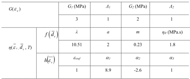
TABLE 1. Model coefficient values

G(e) G1 (MPa) Λ1 G2 (MPa) Λ2 3 1 2 1 η(v,dv, T)

( )

v f d λ a m η (MPa.s) 10.51 2 0.23 1.8

( )

v h vref 1 2 3 1 8.9 -2.6 1

TABLE 2. Sensitivity of coefficients

G1 (MPa) Λ1 G2 (MPa) Λ2 λ a

0.5 4.10-2 0.8 0.2 8.5 2.10-5

m η (MPa.s) vref 1 2 3

LIST OF FIGURES AND CAPTION

Figure 1. Singularity problem using the equation 11 for the h function

Figure 2. (a) Experimental set-up for biaxial test and comparison between experimental results and model simulations for the case 2s-1 _{and 90°C: (b) Constant Width; (c)} Equi-biaxial

Figure 3. Implementation of the model in ABAQUS

Figure 4. (a) Stretch and free blowing of a preform; (b) Abaqus simulation with anisotropic model

Figure 5. Comparison the pressure evolution from experiments and simulation Figure 6. (a) Free blowing like simulation; (b) Stretch blowing simulation

Figure 7. (a) Velocity of the stretch rod; (b) Air mass flow rate as a function of pressure difference (dP)

Figure 8. The distribution of the thickness of the bottle: (a) Free blowing like simulation; (b) Stretch blowing simulation

(a)

(b) (c)

Figure 2. (a) Experimental set-up for biaxial test and comparison between experimental results and model simulations for the case 2s-1 and 90°C: (b) Constant

Figure 4. (a) Stretch and free blowing of a preform; (b) Abaqus simulation with anisotropic model

(a)

(b)

(a)

(b)

Figure 7. (a) Velocity of the stretch rod; (b) Air mass flow rate as a function of pressure difference (dP)

(a) (b)

Figure 8. The distribution of the thickness of the bottle: (a) Free blowing like simulation; (b) Stretch blowing simulation