2006 — Turbomachinery turbine blade vibratory stress prediction

THESIS PRESENTED TO

L'ÉCOLE DE TECHNOLOGIE SUPÉRIEURE

A PARTIAL REQUIREMENT TOOBTAINA

MASTER'S DEGREE IN MECHANICAL ENGINEERING M.Eng.

BY

MARIO GUERRA

TURBOMACHINERY TURBINE BLADE VIBRATORY STRESS PREDICTION

MONTREAL, JANUARY 9rd, 2006

Dr. Marc Thomas Ph.D., thesis supervisor

Mechanical Engineering Department at the École de technologie supérieure

Dr. Éric Davie Ph.D., thesis cosupervisor

Mechanical Engineering Department at the École de technologie supérieure

Dr. Azzeddine Soulaïmani Ph.D., jury president

Mechanical Engineering Department at the École de technologie supérieure

Dr. Henri Champliaud Ph.D., jury member

Mechanical Engineering Department at the École de technologie supérieure

IT WAS DEFENDED IN FRONT OF THE JURY ON NOVEMBER 8, 2005

Mario Guerra

ABSTRACT

The objective of this thesis was to develop a methodology to predict the vibratory stresses of a turbomachinery turbine blade. The aerodynamic excitation phenomenon was not studied in this research. Furthermore, the turbine blades studied in this research had the characteristics of being unshrouded, uncooled and used mainly in small to medium sized turbomachineries.

This thesis consists of four main subjects. The first subject, composed of an analysis of experimental results, was done to ex tract damping values of the turbine blades as well as resonances. The damping values extracted from the experimental data were used to determine analytical vibratory stresses with FLARES. Furthermore, the resonances were identified during the data reduction and therefore, the experimental vibratory stresses were extracted. These values were later used to correlate the analytical vibratory stresses predicted using FLARES.

The second subject elaborated on an analytical method with finite element analysis using contact elements to determine natural frequencies and mode shapes of the turbine blades. The new analysis with contact elements surpassed all expectations with respect to the current analysis being performed at Pratt & Whitney Canada. The natural frequencies were compared with experimental data, and were found to be in good agreement. Furthermore, the mode shapes were compared with the current analysis results, and were found to be identical.

The third subject describes an experimental method to test the blades in a controlled environment to extract natural frequencies, damping and mode shapes. The experimental testing was not performed with great success. The main deficiency was the excitable frequency range created by the high-frequency speaker.

Finally, the fourth subject compares the vibratory stress experimental values and the prediction of vibratory stresses through an analytical tool. Using the FLARES tool, the modal amplification factor was found for every resonance of the PWC Engine 1 HPT Blade, PWC Engine 2 HPT Blade and the PWC Engine 3 CT Blade. Therefore, it can be concluded that the FLARES analytical tool can predict accurate vibratory stress levels due to a resonance for an unshrouded, uncooled turbomachinery turbine blade fairly weiL More work needs to be done on the CFD part of the solution to predict more accurate unsteady pressure levels at the higher engine rotating speeds.

Mario Guerra

SOMMAIRE

Dans le monde de l'aéronautique, le but principal de la recherche et développement est de réduire le poids et augmenter l'efficacité des composantes. Dans les turbomachines, une des composantes principales qui est le sujet de ces recherches est l'aube de turbine. De plus en plus, l'aube de la turbine est sollicitée en réduisant le nombre d'étage de turbine pour le même travail effectué tout en réduisant son poids. Ces aubes de turbine ont plusieurs caractéristiques vibratoires, qui à ce jour, font l'objet de plusieurs recherches avancées. Les vibrations d'une aube de turbine sont un phénomène dû à la rotation de la turbine et aux excitations aérodynamiques. Ces vibrations peuvent tomber en résonance et causer la rupture en haute fatigue d'une ou plusieurs aubes de turbine et peuvent entraîner le bris de la turbomachine pendant un vol.

Depuis plusieurs années, des méthodes empiriques et semi empiriques ont été utilisées pour faire la conception d'aubes de turbine. Ces méthodes se sont avérées inefficaces puisque plusieurs résonances ne sont identifiées qu'une fois la turbomachine testée. Certains outils numériques ont été développés pour déterminer, pendant la conception de l'aube, les résonances et les contraintes. Avec ces outils, il est ainsi possible de s'assurer que les résonances sont à l'extérieur du régime de fonctionnement du moteur. Par contre, cette méthode de conception s'avère trop conservatrice puisqu'il faut souvent changer le profil de l'aube ou augmenter sa masse pour être ainsi capable de modifier les résonances afin qu'elles ne se retrouvent pas dans un régime moteur indésirable. Donc, une méthode analytique doit être développée pour quantifier les valeurs de contraintes aux résonances, pour déterminer si 1' aube de turbine doit être modifiée et pour exclure ces résonances du régime de fonctionnement du moteur. Le sujet de cette thèse est de développer une méthodologie pour prédire les contraintes vibratoires d'une aube de turbine. Il est à noter que ce mémoire portera seulement sur les effets vibratoires de l'aube. La provenance des excitations aérodynamiques ne sera pas traitée dans cette recherche.

Ce mémoire comportera quatre parties principales. Premièrement, une analyse des résultats expérimentaux de tests moteurs pour en retirer 1' amortissement total des aubes ainsi que les contraintes vibratoires associées à chacune des résonances sera présentée. Deuxièmement, une méthode d'analyse par éléments finis avec des éléments de contact

pour en déterminer la déformée modale ainsi que la valeur de 1' amortissement pour chacun des modes. Ces résultats seront comparés avec les résultats obtenus lors des tests moteurs ainsi que les résultats obtenus par les modèles analytiques. Finalement, la méthode de prédiction des contraintes de la réponse forcée de 1' aube ainsi que la comparaison entre les résultats analytiques et expérimentaux seront présentées.

Dans une turbomachine, des excitations périodiques peuvent être générées à partir de plusieurs composantes internes dû à la nature rotative du moteur. Donc, lorsqu'une aube de turbine est dans la phase de conception, une attention particulière doit être portée sur ces excitations périodiques, surtout pour le stator placé en amont de la turbine, afin qu'ainsi aucune résonance n'ait lieu dans la zone d'opération normale de la turbomachine. Lors de la réduction des données expérimentales, une résonance peut être identifiée par sa très haute amplitude de contrainte comparée aux restes des fréquences et des vitesses de rotation (Figure 4). Plusieurs résonances peuvent être identifiées pour chaque mode à une fréquence naturelle spécifique, puisqu'il y a plusieurs sources d'excitations ainsi que leurs harmoniques.

Pour déterminer l'amortissement total de l'aube de turbine c-à-d., l'amortissement mécanique (matériel, frottement, etc.) et l'amortissement aérodynamique, les résultats expérimentaux seront utilisés. Cette méthode consiste à isoler la résonance identifiée pour ensuite faire épouser une courbe théorique sur celle obtenue expérimentalement. De cette façon, il sera possible d'en retirer l'amortissement total.

Les contraintes vibratoires aux résonances ainsi que l'amortissement total associé ont été obtenus pour les aubes de type Turbine de Compresseur (TC) ou Turbine à Haute Pression (THP) pour les moteurs suivant : PWC Moteur 1, PWC Moteur 2 et PWC Moteur 3. Ces valeurs d'amortissement seront utilisées pour déterminer analytiquement les contraintes vibratoires avec l'utilisation du logiciel FLARES [2]. De plus, les contraintes vibratoires trouvées serviront à titre de comparaison et calibration aux valeurs de contraintes vibratoires prédites par FLARES.

Le chapitre 4 portera sur l'application de conditions limites utilisant des éléments de contact pour déterminer les caractéristiques dynamiques d'une aube de turbine dans un environnement où le phénomène de friction est présent. Cette étude a été entreprise avec les éléments de contact disponibles dans le logiciel d'éléments finis ANSYS®. Les éléments de contact sont maillés sur toute 1' aire de fixation de 1' aube et du disque de la turbine pour simuler l'interaction entre les faces de contact. Aucune hypothèse n'est émise initialement sur la zone de contact entre 1' aube et le disque. Les éléments de contact du logiciel ANSYS® utilisés nécessitent les valeurs des coefficients de friction dynamique et statique et d'autres paramètres qui auront un effet sur la vitesse de convergence du modèle. Avant d'effectuer l'analyse modale, une analyse statique non linéaire est effectuée en incluant les effets de précontraintes, c-à-d., la température du métal de l'aube ainsi que la vitesse de rotation de la turbine. Cette analyse statique, dite non linéaire à cause de l'ajout des éléments de contact, calcule la nouvelle position

d'équilibre de 1' aube par rapport au disque dû aux effets de précontraintes. Avec la nouvelle position d'équilibre, une analyse modale, nécessairement linéaire, est effectuée dans le but de déterminer les fréquences naturelles ainsi que les déformées modales de l'aube de turbine analysée. Les quatre (4) premières fréquences naturelles de l'aube de turbine sont extraites et évaluées dans cette étude. Une étude de convergence est aussi effectuée pour déterminer quels sont les paramètres des éléments de contact qui ont la plus grande influence sur la valeur des fréquences naturelles. Les résultats expérimentaux sont extraits des tests moteurs pour les fréquences naturelles et de tests de scan laser pour les déformées modales. Il a été déterminé que le nouveau type d'analyse en utilisant des éléments de contact a surpassé toutes les attentes comparées avec l'analyse courante effectuée chez Pratt & Whitney Canada. Les fréquences naturelles ont été comparées avec les données expérimentales. La comparaison montre que les résultats analytiques et expérimentaux sont très similaires. De plus, les déformées modales, obtenues par l'analyse avec les éléments de contact, sont très comparables à l'analyse courante. Aussi, les contraintes déterminées dans les zones de contact entre les aubes et le disque ont diminué d'intensité comparée à l'analyse courante, dont une meilleure prédiction des contraintes vibratoires est à prévoir dans ces zones. Il a aussi été observé que l'aire des zones de contact augmente lors de l'analyse statique avec les effets de précontraintes, ce qui aura une signification importante pour les conditions limites du modèle pendant l'analyse modale. Finalement, une étude de convergence a été effectuée sur cinq paramètres modifiables des éléments de contact. Il a été trouvé que le modèle est stable et convergent. Par contre, la valeur du coefficient de friction a un effet significatif sur la valeur des fréquences naturelles. Des tests de pénétration entre 1' aube et le disque de turbine devraient être effectués pour obtenir des valeurs expérimentales et les comparer avec les valeurs obtenues analytiquement. De plus, une étude devrait être effectuée pour déterminer si le coefficient de friction est identique ou différent pour chacun des modes de la même aube de turbine.

Pour effectuer les tests expérimentaux, une aube et un disque de turbine d'un moteur seront utilisés. Pour faire une bonne corrélation entre les résultats expérimentaux et analytiques, les conditions limites devront être très similaires. Pour les tests expérimentaux, 1' aube de turbine sera assemblée dans le disque. Le disque sera soutenu par un montage spécialement conçu pour éviter ses propres fréquences de résonances dans la zone d'intérêt. Pour simuler l'effet de la force centrifuge, deux vis seront serrées dans le chanfrein du trou pour le rivet, ce qui créera une force verticale (Figure 11). Pour recréer les mêmes conditions limites sur le modèle analytique, la force centrifuge a été remplacée par un déplacement de 0,1 pouce (valeur approximative) dans le chanfrein du trou pour le rivet, dans les directions axiale et radiale (Figure 12). Lorsqu'on effectue une analyse modale expérimentale, normalement un marteau est utilisé pour exciter la composante et un accéléromètre est utilisé pour enregistrer le signal de réponse de la composante. Ceci n'est pas un problème lorsque la composante a une masse beaucoup plus significative que l'accéléromètre. Dans notre cas, l'aube de turbine a une masse inférieure à dix (10) fois la masse de l'accéléromètre. Donc, pour éviter un changement

PolyTec sera utilisé (Figure 13). Le vibromètre au laser enregistrera neuf (9) points différents sur l'aube de turbine. De cette façon, la déformée modale sera créée avec une plus grande précision (Figure 14). Pour exciter l'aube de turbine, au lieu d'un marteau typique, un haut-parleur à haute fréquence, modèle JBL Série Professionnel No. 2425, couplé à un cône, modèle No. 2306, sera utilisé (Figure 15). Un générateur de fréquence sera utilisé pour créer un signal sinusoïdal avec une plage de 2000 à 20 000 Hz. Le générateur de fréquence est branché à un mixeur Mackie Série Micro 1202-VLZ et ensuite à un amplificateur TOA Corporation Dual Power Amplifier Model: IP-300D duquel la sortie est branchée au haut-parleur à haute fréquence JBL. Le système d'acquisition de données utilisé est un Zonic Médaillon, avec 8 canaux de 0 à 20kHz. La sortie en vitesse du vibromètre au laser est directement branchée à un des canaux du système d'acquisition de données. La sortie du haut-parleur est captée par un microphone avec une extrême sensibilité qui est placé très près de l'aube de turbine. Le microphone est branché à un des canaux du système d'acquisition de données. Les paramètres du système d'acquisition de données sont modifiés pendant les tests expérimentaux pour obtenir la meilleure résolution en fréquence pour la plage de 2000 à 20 000 Hz. Le logiciel d'acquisition de données génère une fonction de réponse en fréquence (F.R.F.) en divisant le signal provenant du vibromètre par le signal provenant du microphone. Les parties réelle et imaginaire de la F .R.F. seront utilisées pour déterminer les fréquences naturelles et la déformée modale associée.

Les tests expérimentaux n'ont pas été concluants. Le problème principal était que la plage de fréquence excitée n'était pas assez large pour avoir un signal pour tous les modes. Le haut-parleur, JBL Série Professionnel Modèle No. 2425, couplé à un cône, Modèle No. 2306, avait la capacité d'exciter une plage de fréquence allant de 3500 à 8000 Hz. Les prédictions analytiques démontraient que les quatre premiers modes de l'aube de turbine testée étaient dans la plage de fréquence allant de 3000 à 17 000 Hz. Donc, les résultats pour les modes 2, 3 et 4 sont questionnables. De plus, la cohérence du signal montrait des lacunes à de multiples fréquences dues au manque d'excitation provenant du haut-parleur. Par contre, 9 modes ont été extraits des données expérimentales. Les quatre modes analytiques ont très bien corrélé avec les résultats expérimentaux en terme de fréquence naturelle et de déformée modale. Par contre, puisque les données expérimentales sont questionnables, dues à la petite plage de fréquences excitées, l'extraction de l'amortissement modal n'a pas été effectuée.

Les aubes de turbine sont sujettes à des contraintes vibratoires dues à des écoulements turbulents dans la trajectoire des gaz de la turbomachine. La turbulence dans l'écoulement induit différentes forces sur l'aube de turbine. Lorsque la fréquence de l'instabilité est égale avec une des fréquences naturelles de l'aube, une résonance est créée avec laquelle de hautes contraintes vibratoires sont associées. Cette problématique est aussi appelée l'aéroélasticité. Plusieurs sources d'écoulement instationnaire existent dans une turbomachine, comme :

)o> Sillage d'aube de turbine 1 de stator

>

La plupart des écoulements instables sont circonférentiellement périodiques et sont des multiples de la vitesse de rotation de la turbomachine.

Pour prédire analytiquement les contraintes vibratoires d'une aube de turbine, la solution de l'analyse modale ainsi que la solution de la dynamique du fluide (FD) à la vitesse de rotation où la résonance est située, doivent être couplées. La solution FD n'est pas présentée dans cette étude, mais en résumé, une solution FD Euler est exécutée pour déterminer l'écoulement permanent et ainsi calculer l'amortissement aérodynamique. La partie instable de l'écoulement est déterminée avec les équations de Navier Stokes où un modèle turbulent est introduit dans le modèle. Les solutions de l'écoulement stable et instable (vs. temps) sont requises pour déterminer la force aérodynamique sur l'aube de la turbine.

En utilisant le logiciel FLARES, le facteur d'amplification modal a été obtenu pour chacune des résonances des aubes de turbine des moteurs PWC Moteur 1, PWC Moteur 2 et PWC Moteur 3. Pour déterminer les contraintes vibratoires, la matrice des contraintes vibratoires obtenues lors de l'analyse modale pour une résonance particulière est multipliée par le facteur d'amplification modal obtenu avec FLARES. La matrice de contrainte vibratoire est déterminée avec ANSYS en utilisant la valeur maximum des contraintes S1 ou S3 à chacun des nœuds et ensuite en affichant les valeurs à l'échelle. Pour s'assurer de la validité des résultats, la déformée modale extraite par FLARES a été comparée à la déformée modale obtenue avec ANSYS. De plus, l'ampleur de la force modale a été révisée pour chacune des harmoniques de l'excitation. Après investigation, il a été déterminé que le code FD ne pouvait pas prédire l'écoulement instationnaire à très haute vitesse due à des effets non linéaires basés sur le nombre de Reynolds. Donc, le niveau des contraintes vibratoires, dues à la résonance entre le deuxième mode et la première harmonique de 1' excitation provenant du stator en amont, a été prédit avec une marge d'erreur allant de 0% à 371%. Le niveau des contraintes vibratoires, due à la résonance entre le quatrième mode et la deuxième harmonique de 1' excitation provenant du stator en amont, a été prédit avec une marge d'erreur allant de 0% à 94%. Donc, en résumé, l'outil analytique FLARES peut prédire des contraintes vibratoires avec une bonne précision pour des aubes de turbine sans refroidissement. Par contre, plus d'études sont nécessaires sur la solution aérodynamique pour prédire des niveaux de pression instationnaire plus correctement à des vitesses de rotation très élevée de la turbomachine.

En conclusion, cette thèse comportait quatre aspects importants. Le premier objectif a été d'extraire des données expérimentales, les résonances, les contraintes vibratoires et les amortissements totaux. Cet objectif a été atteint grâce à l'élaboration d'un programme MATLAB pour extraire l'amortissement total. Le deuxième objectif a été d'élaborer un nouveau modèle par élément finis pour déterminer les fréquences

éléments de contact pour simuler l'interaction entre l'aube de turbine et le disque, cet objectif a aussi été atteint. Le troisième objectif a été de déterminer les fréquences naturelles, les déformées modales et l'amortissement mécanique d'une aube à l'aide d'un banc d'essai expérimental. Cet objectif n'a pas été atteint du à la petite plage de fréquence d'excitation. Finalement, le quatrième objectif a été de prédire les contraintes vibratoires analytiquement d'une aube de turbine. Avec l'utilisation du logiciel FLARES, cet objectif a été atteint puisque les contraintes vibratoires prédites ont été comparées avec les résultats expérimentaux avec un pourcentage d'erreur acceptable.

I would like to express my gratitude towards my supervisor, Dr. Marc Thomas, and co-supervisor, Dr. Eric David, for their support and teachings. Without their help, this study would have taken far longer to be completed. Futhermore, the jury members should be noted for their time and effort to make this thesis more complete.

I would like to acknowledge my coworkers at Pratt & Whitney Canada for their help and support on this project. Hopefully, this work will help us understand more about turbine blades and therefore improve our design activities.

Also, I would like to thank the« Centre de Recherche Industriel du Quebec » (CRIQ) for their help and donation of the high-frequency speaker used during the experimental tes ting.

Finally, I would like to specially thank my fiancée for ali of her support and help throughout this endeavor.

Page ABSTRACT ... i SOMMAIRE ... ii ACKNOWLEDGEMENT ... viii TABLE OF CONTENTS ... ix LIST OF TABLES ... xi

LIST OF FIGURES ... xii

LIST OF ABBREVIATIONS AND SYMBOLS ... xv

INTRODUCTION ... 1

CHAPTER 1 LITTERATURE REVIEW ... 3

CHAPTER 2 OBJECTIVES AND METHODOLOGY ... 9

CHAPTER 3 STRAIN GAGE TEST DATA EXTRACTION ... 11

3.1 Resonance Identification ... 11

3.2 Modal Damping Extraction ... 13

3.3 Vibratory Stress Calculation ... 17

CHAPTER 4 FINITE ELEMENT MODEL BOUNDARY CONDITIONS DEFINITION ... 19

4.1 Current Analysis ... 20

4.2 New Analysis ... 22

4.3 Meshing of Contact Elements ... 22

4.4 Contact Element Input Data ... 25

CHAPTER 5 EXPERIMENTAL TESTING ... 27

5.1 Experimental Test Model ... 27

5.2 Response Signature Recording ... 29

5.3 Excitation ... 31

5.4 Data Acquisition ... 32

CHAPTER 6 VIBRA TORY STRESS ANALYTICAL PREDICTON ... 33

6.1 FLARES Analytical Tool ... 34

7.1 Strain Gage Test Data Reduction Results ... 38

7 .1.1 Resonance results ... 3 8 7 .1.2 Modal damping extraction results ... .40

7 .1.3 Experimental vibratory stress results ... 42

7 .1.4 Discussion on the strain gage data reduction results ... .43

7.2 Results ofthe Updated Boundary Conditions Analyses ... .44

7.2.1 Comparison between the current and the new analyses ... .44

7 .2.2 Convergence study ... 46

7 .2.3 Analytical results using contact elements modal analysis ... 50

7.3 Experimental Tests Results ... 59

7.4 Analytical Vibratory Stress Prediction Results ... 70

7.4.1 Results verification ... 70

7.4.2 Modal amplification factor results ... 72

7.4.3 Analytical vibratory stress results interpretation ... 72

CONCLUSION ... 76

APPENDICES 1 : DampingExtractionMA TLABProgram ... 79

2 : Engine Resonant Frequencies Results ... 84

3 : Engine Modal Damping Results ... 88

4 : Engine Vibratory Stress Results ... 90

5 : JBL Speaker Specifications ... 94

6 : FLARES Input File ... 96

7: Engine Vibratory Stress Analytical Prediction Results ... 101

Page

Table I MATLAB® routine inputs ... 16

Table II Contact type for the static and modal analyses ... 24

Table III PWC Engine 1 Resonant Frequencies ... 39

Table IV PWC Engine 1 Modal damping ... .40

Table V PWC Engine 1 Vibratory Stress ... .42

Table VI PWC Engine 1 HPT Blade Natural Frequency Comparison @ 35200 RPM ... 51

Table VII PWC Engine 1 HPT Blade Natural Frequency Comparison @ 33000 RPM ... 52

Table VIII PWC Engine 2 HPT Blade Natural Frequency Comparison @ 33289 RPM ... 54

Table IX PWC Engine 2 HPT Blade Natural Frequency Comparison @ 30000 RPM ... 55

Table X PWC Engine 3 CT Blade Natural Frequency Comparison @ 43000 RPM ... 56

Table XI PWC Engine 3 CT Blade Natural Frequency Comparison @ 36000 RPM ... 58

Table XII Resonances and Imaginary values for every location ... 63

Table XIII Experimental and Analytical natural frequencies comparison ... 68

Table XIV PWC Engine 1 HPT Blade Analytical Vibratory Stress Comparison ... 72

Table XV PWC Engine 2 Resonant Frequencies ... 85

Table XVI PWC Engine 3 Resonant Frequencies ... 87

Table XVII PWC Engine 2 Modal Damping ... 89

Table XVIII PWC Engine 3 Modal Damping ... 89

Table XIX PWC Engine 2 Vibratory Stress ... 91

Table XX PWC Engine 3 Vibratory Stress ... 93

Table XXI PWC Engine 2 Analytical Vibratory HPT Blade Stress Comparison ... 102

Figure 1 Figure 2 Figure 3 Figure 4 Figure 5 Figure 6 Figure 7 Figure 8 Figure 9 Page Aerodynamic excitation ... 4

Solid versus foundation ... 5

Method to predict the forced response of a turbine blade ... 8

Waterfall 0-25000 Hz ... 12

Resonance spectrum plot ... 14

Curve fitting for damping extraction ... 17

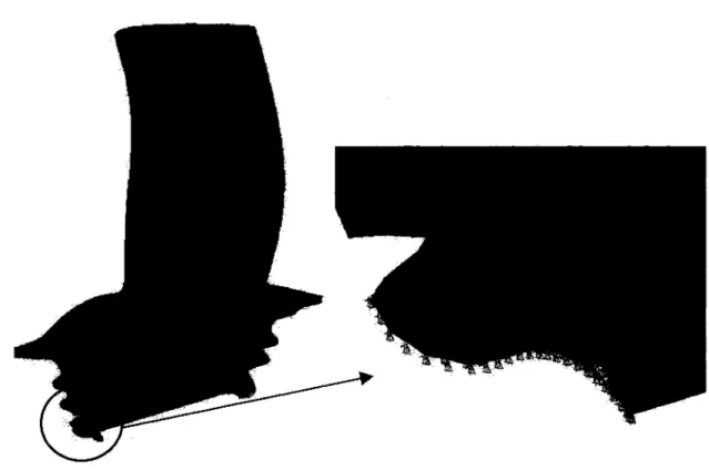
Blade fir-tree line blockage ... 20

Blade stress with contact lin es blocked ... 21

Blade and dise meshing ... 23

Figure 1 0 Contact elements mesh ... 24

Figure 11 Experimental test mount simulation of centrifugai force ... 28

Figure 12 FEM model experimental boundary conditions ... 29

Figure 13 PolyTec Laser Vibrometer ... 30

Figure 14 Blade signal recording locations ... 30

Figure 15 JBL Professional Series Model No. 2425 High Frequency Speaker coupled to Model No. 2306 Hom ... 31

Figure 16 Harmonie damping trend vs. Airfoil wetted area ... 41

Figure 17 Current analysis mode shape ... 45

Figure 18 New analysis mode shape ... 45

Figure 19 Blade stress in the fir-tree area (Inside the airfoil's cooling pocket) ... .45

Figure 20 Contact face width ... 46

Figure 21 Frequency error vs. friction coefficient ... .47

Figure 22 Frequency vs. Normal contact stiffness factor ... 48

Figure 24 Frequency vs. Ratio between the static and dynamic friction coefficient

and the slip rate decay coefficient ... 50

Figure 25 PWC Engine 1 HPT Blade Natural Frequency Comparison @ 35200 RPM ... 52

Figure 26 PWC Engine 1 HPT Blade Natural Frequency Comparison @ 33000 RPM ... 53

Figure 27 PWC Engine 2 HPT Blade Natural Frequency Comparison @ 33289 RPM ... 54

Figure 28 PWC Engine 2 HPT Blade Natural Frequency Comparison @ 30000 RPM ... 55

Figure 29 PWC Engine 3 CT Blade Natural Frequency Comparison@ 43000 RPM .. 57

Figure 30 PWC Engine 3 CT Blade Natural Frequency Comparison@ 36000 RPM .. 58

Figure 31 Excitation Autospectrum for excited frequency range ... 59

Figure 32 Example of a Coherence signal.. ... 60

Figure 33 Example F.R.F. signal Imaginary part for mode shape and damping determination ... 61

Figure 34 Example F .R.F. signal Real part for natural frequency determination ... 62

Figure 35 Exp. Mode 1@ 4689.6Hz ... 64

Figure 36 Mode 1@ 4935 Hz ... 64

Figure 37 Exp. Mode 2@ 7652.7 Hz ... 65

Figure 38 Exp. Mode @ 8272 Hz ... 65

Figure 39 Exp. Mode 4@ 9415.3 Hz ... 65

Figure 40 Exp. Mode 5@ 10830.7 Hz ... 66

Figure 41 Exp. Mode 6@ 11474.7 Hz ... 66

Figure42 Mode2@11675Hz ... 66

Figure 43 Exp. Mode 7@ 12497.9 Hz ... 66

Figure 44 Exp. Mode 8@ 14306.1 Hz ... 67

Figure 45 Mode 3@ 15193 Hz ... 67

Figure 46 Exp. Mode 9@ 16803.9 Hz ... 67

Figure47 Mode4@ 16638 Hz ... 67

Figure 48 Excitable range on the JBL High Frequency Speaker ... 69

Figure 50 Modal force versus the harmonie of the unsteady pressure signal generated by FLARES ... 71

HPT CT HCF CFD SDOF SGT CF MU FKN FTOLN FACT DC P&WC FEM F.R.F. WF EO OA

[C]

High pressure turbine Compressor turbine High cycle fatigue

Computational fluid dynamics Single degree of freedom Strain gage test

Centrifugai force

Dynamic coefficient of friction Contact stiffness factor

Penetration tolerance factor

Ratio between the static and dynamic coefficient of friction Decay coefficient

Pratt & Whitney Canada Finite element model

Frequency response function Waterfall

Engine order Overall

Structural damping matrix

Equivalent static stress or strain (static deflection) F The modal amplification factor

{F} Nonlinear centrifugai force vector

{F(u, .Q)}

[K] Geometrically nonlinear stiffness matrix including centrifugai stiffness and softening

L

[M]

{q}

{u}

Structural mass matrix Resonance speed (RPM) Rotor speed (RPM)

Nonlinear aerodynamic force vector

Aerodynamic forces from the normal modes. Normal or modal coordinates

Time (sec)

Structural position vector Time-averaged position

{u

{P(u)}

{.PM (u,

{.PG

t)}

In aeronautics, the main goal in research and development is to reduce weight and increase components efficiency. In turbomachinery, one of the main components for which a lot of research is performed is the turbine blade. The turbine blade is more and more excited by reducing the number of turbine stages required to perform the same work as well as reducing its weight. The turbine blades have multiple vibratory characteristics that have aroused many advanced research projects. The turbine blade vibrations are caused by the rotation of the blade and aerodynamical excitations. These vibrations can cause failure in high cycle fatigue (HCF) of one of multiple blades by entering in resonance, which can also cause damage to the engine and could result in an in-flight shutdown. According to the NASA/GUide Consortium Industry Survey [1], one in-flight shutdown can cause monetary damages ranging from 500 000 to 4 000 000 $. It

is also noted that 14% of engine development difficulties are due to turbine blade vibrations. Furthermore, one engine in development encounters on average 2.5 serious blade vibration problems. It is therefore easy to understand the need for studies performed on turbine blade vibrations.

For many years, empirical and semi-empirical methods have been used to design turbine blades. These methods were found to be ineffective since multiple resonances were identified only after the engine was tested. Multiple numerical tools have been developed to determine, during the design phase of turbine blades, the resonances and vibratory stresses. With these tools, it is possible to determine, with little doubt, if the resonances will be outside the normal operating range of the turbomachinery. On the other hand, this method was found to be too conservative since changes must be made to the blade to tune out resonance so that they are not situated in the operating range of the engine. Therefore, an analytical methodology must be developed to quantify vibratory stresses of a turbine blade at resonance, and to determine if the blade must be modified or will be within the material HCF capabilities. The subject of this thesis will be to develop a methodology to predict the vibratory stresses of a turbomachinery turbine

blade. It is noted that this thesis will only treat the vibratory stresses of a turbine blade. The aerodynamic excitation phenomenon will not be seen in this research. Furthermore, the turbine blades studied in this research will have the characteristics of being unshrouded, uncooled and used mainly in small to medium sized turbomachineries.

This thesis consists of four principal subjects. The first subject composed of an analysis of experimental results, which will be done to extract damping values of the turbine blades as well as resonances. The second subject will elaborate on an analytical method with finite element analysis using contact elements to determine natural frequencies and modes shapes of the turbine blades. The third subject will discuss an experimental method to test the blades in a controlled environment to extract natural frequencies, damping and mode shapes. Finally, the fourth subject will compare the vibratory stress experimental values with the prediction ofvibratory stresses through an analytical tool.

LITERATURE REVIEW

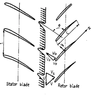
Numerous scientists have studied the unsteady aerodynamic excitation phenomenon during the past years. As per Hilbert et al. [2], the unsteady aerodynamic forces are obtained by three major sources. The first source of unsteadiness is due to the interaction between the rotating turbine blades and the turbine stator vanes. Furthermore, the circumferential non-conformities such as flow loss for other means ( cooling) and the variations in the blade tip clearances are also sources of unsteadiness. The second source of flow unsteadiness cornes from the turbine blade vibration adjacent to the studied blade. The third and last major source of flow unsteadiness cornes from the vortex created by the blades and vanes situated upstream and downstream of the turbine blade set. Ishiara [3] performed experimental and analytical studies on the blade vibration phenomenon by concentrating his efforts on the flow unsteadiness caused by the interaction between the stator vanes and the turbine blades. To perform his study, Ishihara assumed the following three hypotheses: the two dimensional flow is incompressible, the flow instability and the blade vibrations cause the unsteady aerodynamic forces, and the speed of the flow fluctuation is inferior to the flow average speed (Figure 1 ).

Stator blade

Figure 1 Aerodynamic excitation1

Hilditch et al. [ 4] performed studies on the unsteady pressures and the heat transfer of high-pressure turbines. They compared their experimental results with analytical results obtained from the program code UNSFLO. UNSFLO is a numerical simulation code to obtain results of two-dimensional unsteady pressures and it is used by multiple companies that design and build turbomachine engin es. Krysinski et al. [ 5] also performed studies on three-dimensional unsteady flows. They experimentally investigated the effects on the performance of the turbine blades in regards to the angular positioning of the stator vanes. Jocker et al. [6] performed studies on the influence of certain parameters of the parametrical excitations caused by the stator vanes on the high pressure turbine blades. Clark et al. [7] performed Computational Fluid Dynamics (CFD) analyses in three dimensions during the design process of a turbine blade with the goal of predicting with more accuracy the unsteady aerodynamic forces.

A chapter of this thesis will define a finite element model using contact elements to predict the natural frequencies and mode shapes of a turbine blade. Meguid et al. [8] performed analyses with finite element modelling of the turbine fixation zone. However, these analyses were performed in the static domain to obtain the stress patterns and values. They compared their results with experimental results provided by photo-elastic testing. The type of contact elements that will be used are the ones available in ANSYS® and therefore will only be the ones used in this thesis. The contact elements that will be used must be three-dimensional and must be able to consider the friction phenomenon. The friction contact elements used in ANSYS® are based on the mixed variational principles. Cescotto et al. [9] have presented an original approach to the numerical modelling of unilateral contact by the finite element method. The alternative solution that Cescotto et al. have found was to discretize independently the contact stresses and the displacement field on the solid boundary. « It is based on a mixed variational principles and allows controlling the average overlapping between the solid boundary and the foundation. In other words, a node which is not yet in contact but only close to the contact is 'informed' by its neighbours that contact is going to occur soon. »2 (Figure 2)

Deformable solid

Gauss integration _ /

pain!

RigidJdeformatJie body

Figure 2 Solid versus foundation

« The finite elements are based on the penalty method for solving the unilateral contact and slip conditions and on the Coulomb model for the friction strength. When slipping contact appears, the constitutive equation of the contact element is unsymmetrical. Therefore, an unsymmetrical solver is used. »3 This method is currently being used in ANSYS® to solve model which uses contact elements. In addition, Berger et al. [10] created a user-programmed function in ANSYS® to perform analyses of microslip damping on a turbine blade. They have created a "superelement" that would replace the contact elements currently used in ANSYS®. This new element contains a friction traction law definition based on the Coulomb friction model and a stick-slip transition logic based upon the force and velocity conditions. Although is still uses the contact elements from ANSYS® to determine the initial contact phase, the computational time per load step is greatly reduced. The overall energy dissipation, stresses and interface tractions are more accurately predicted. There are two reasons for which this methodology will not be used in this thesis. First, this macro is not yet available for the public. Second, the "superelement" in a two dimensional problem, while the fixing a turbine blade is a three dimensional problem.

A chapter of this thesis will describe a modal testing procedure to determine the natural frequencies and mode shapes of a turbine blade using an acoustical excitation. Li et al. [ 11] performed such experiments on an ad vance bladed disk prototype. The reason for an acoustical excitation is to produce a non-contacting measurement system and therefore, not affecting the system response. The measurement of the excitation is done using a calibrated microphone, while the measurement of the disk response is done with a Single-Point Laser Vibrometer (SPLV) and a Scanning Laser Doppler Vibrometer (SLDV). The speaker generates a signal, which excites the disk blades at their natural frequencies. Using the microphone, the sound pressure level is recorded so that a Frequency Response Function can be obtained. Li et al. used a travelling excitation wave

to excite ali the blades of the disk. In this thesis, only one blade will be tested and therefore, a single speaker excitation will be needed.

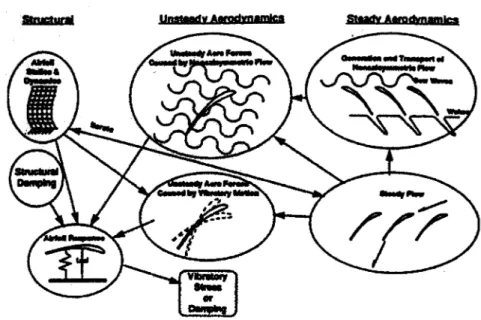
Jay et al. [12] performed studies on turbine blades forced response. By performing experimental testing, they were able to identify the dynamic responses resulting from the interaction between the stator vanes and the turbine rotor blades. Furthermore, they performed an analytical description of the aerodynamic force originating in the difference between the number of stator vanes and the number of turbine blades. Moffatt et al. [13] also performed the same studies as Jay et al. [12], although using the program ANSYS® to determine the natural frequencies and mode shapes of the studied turbine blade and interpolated the results with the CFD meshing. The Navier-Stokes equations were resolved in the frequency domain by using a one-vane passage approach to obtain the aerodynamic excitation and the damped forces. This method was based on single-degree-of-freedom (SDOF) assumptions. Ultimately, Hilbert et AL [2] performed the same studies on forced response in a three-dimensional field. The analysis consisted in a three-dimensional multi-stage turbine in which the stable and unstable dynamic fluid response was determined. A non-linear structural analysis and a linear dynamic analysis were performed to determine the displacement amplitude of the blade in resonance during the engine run. By combining a structural analysis and a dynamic analysis with a the fluid dynamic analysis, an iterative solution to the aeroelastic problem was obtained (Figure 3).

Figure 3 Method to predict the forced response of a turbine blade4

Busby et Al. [14] already performed studies on the axial blade spacing effect and determined that the increase in total relative pressure loss of the turbine blade was eliminated by the decrease in total relative pressure loss of the stator vane when the axial spacing was decreased. Furthermore, the predicted decrease in pressure loss of the stator vanes with the decrease in the axial spacing is mainly due to the reduction in wake mixing loss. Finally, the predicted increase in the total relative pressure loss of the turbine blade with a decrease of the axial spacing is mainly due to the increased interaction between the wakes produced by the stator vanes with the turbine blades.

OBJECTIVES AND METHODOLOGY

The forced response prediction, with accuracy, of the turbomachinery turbine blade forced response will be studied throughout this thesis. The turbine blades studied will be uncooled and unshrouded. The thesis objectives will be the following:

~ Extract the total damping based on experimental data.

~ Create a fini te element model using contact elements for more accurate boundary conditions.

~ Experimentally measure the natural frequencies, modes shapes and mechanical damping values.

~ Create a methodology to predict vibratory stresses in the turbine blade.

To extract the total damping of the turbine blade, meaning the mechanical damping (material, friction, etc.) and the aerodynamical damping, the experimental data from previous tests will be used. This method consists in isolating the identified resonance and fit a theoretical curve over the experimental data. Using this theoretical curve, the total damping will be extracted. For the finite element model, a three-dimension turbine blade model and part of the dise will be meshed. No hypothesis will be made on the localization of the contact surface between the turbine blade and the dise. Therefore, the who le fixation zone of the blade and the dise will be meshed with contact elements. The fini te element model will determine the natural frequencies and the mode shapes of the turbine blade. The analytical results will be compared to the experimental results. For the experimental testing, a laser vibrometer and an acoustic excitation will be used to determine the natural frequencies, modes shapes and extract the mechanical damping values. For the prediction of the vibratory stresses method, the FLARES [2] code will be used to superimpose the aerodynamic forces onto the turbine blade. From this, the modal participation factor will be obtained. This factor will multiply the modal stress vector obtained by the fini te element model so that, finally, the vibratory stresses of the turbine

blade can be obtained. Most of the work will be on the parametric study to obtain consistent stress values from FLARES and ANSYS®.

STRAIN GAGE TEST DATA EXTRACTION

Experimental data has to be extracted from a Strain Gage Test (SGT) so that HCF (High Cycle Fatigue) lifing can be performed on the required blade. In addition, in this research project, the experimental data has to be extracted so that it can be correlated with the analytical results. Furthermore, to obtain the vibratory stresses analytically, the damping value has to be extracted from the data reduction since it cannot, currently, be calculated analytically. The data reduction will be done only on the high-pressure turbine blade for turbofans engine and the compressor turbine blade for the turboprops engin es. The data reduction will be performed on the high-pressure turbine blade of the PWC Engine 1 and PWC Engine 2 engines, and on the compressor turbine blade of the PWC Engine 3 engine. These blades are uncooled, unshrouded (no inter-connection between blades) and the data extrapolated are only to be used on blades with the same characteristics for design. Furthermore, a damping value trend will be extrapolated as function of mode, natural frequency and harmonie of excitation. It is important to note that only the modes that are in resonance or close to will be of importance and studied.

3.1 Resonance Identification

A resonance is defined as a coïncidence between a natural frequency of a component and a periodic excitation on a waterfall (Figure 4). A waterfall is obtained from a Fast Fourier Transform of a time signal given by a strain gage during an engine testing. The three axes represent the following: the frequency range, the engine rotational speed and the amplitude of the vibratory strain. Every horizontalline represents one capture engine speed during the test. During the test, the strain gage captures the vibratory strain at the determine location on a blade. The blade exhibits vibratory strain due to its own natural frequencies ( almost parallel to the engine rotational speed axis) or due to the excitation sources. If the excitation is an integer of the rotation speed, such as upstream vane

wakes, a diagonalline will appear on the waterfall. If the excitation line and the natural frequency line meet, a resonance will occur which is usually demonstrated by high amplitude vibratory strain.

84851111 1 Accel to first li mit (0->end) ENG:621186 T/C:22- 01 1 3- MAR- 2003 20:45:22 JE WF 0-25000Hz N2 ( SPECACQ 0-25600Hz R/601/1/6464) dt•0.101sec 3E ue PEAK (rms.x1.414) Figure 4 Waterfall 0-25000 Hz 36000

In a turbine engine, periodic excitations can be generated by multiple components due to the rotating nature of the engine. Therefore, when designing a turbine blade, great care must be taken to the periodic excitations, mostly the vane passing, so that no resonance occur in the running range of the engine. When performing data reduction, resonance can be identified by the high amplitude of the strain compared to the rest of the frequencies and rotating speeds (Figure 4). Multiple resonances can be identified on each mode at specifie natural frequency due to the different surrounding components and the excitation harmonies. The results are presented in section 7 .1.1.

3.2 Modal Damping Extraction

When turbine blade vibratory stresses are predicted analytically, the total damping acting on the blade is cri ti cal to the accuracy of the stress value. The total damping is the sum of the aerodynamic damping and the mechanical damping. Furthermore, the mechanical damping comprises the structural damping of the material and the friction damping generated in the fixing area. These quantities depend on the CF load, metal temperature, frequency, material and surface finish at the blade-disc interface. The aerodynamic damping can be obtained by analytical calculations using Euler equations. As for the remaining damping values, the only accurate method to obtain them is from experimental testing. Therefore, from SGT data reduction, the total damping values have to be extracted so that the stress values can be predicted with accuracy.

The basic method to determine the total damping value is the following: 1- Identification of the resonance

2- Identification of the Engine Order range 3- Export the data

4- Curve fitting 5- Analytical tool

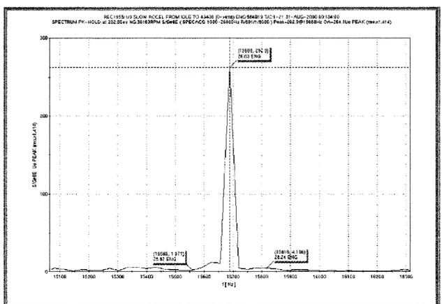
The identification of the resonance was presented previously (Figure 4). The goal of the Engine Order Plot is to build the blade response versus the rotor speed on an engine order excitation in order to have almost a constant force over a small rotor speed range. The Engine Order band has to be wide enough to capture the severa! adjacent spectral components that define the full peak. To make sure that the Engine Order Plot range is wide enough, a spectrum plot at the resonance speed is plotted from the waterfall (Figure 5).

,.

i

R~C 1955iu$ SLOW ACCH H:OM IOLE TO 4U.OO (0-:.enu~ ~N(dili491 g 1Jr.::·t -l1 31 -.~UG-2000 fii)·1S4:110

SPEC1AIJM Pt.:-HOI.to a1 2:$.2:.QS~t: t~G:,Eo163RPM Sr'Gt6G ~ S.PEC-P.CO 1000-2:6000Hz Pie[l1f1rtl0DO) peat; .. fi2,g~156e&Hz OA-.2:64.1UE< F'EAK(rme)'ïi.414)

)00.---~---~---~---~----~---.

'"'

i

Figure 5 Resonance spectrum plot

Based on the spectrum plot, the Engine Order band is defined by incorporating the whole peak. The Engine Order Plot is relative to the engine rotor speed. To get the real resonant peak, an average over a frequency bandwidth for each engine revolution is done. To avoid any loss of information, the FFT frequency bandwidth has to be centered on the resonance frequency and has to be equal or less than 6400 Hz due to the limitation in resolution of the analyzer. Using this information, the data can be exported to an ASCII file for post-processing.

In order to extract the damping from the Engine Order curve, a single degree of freedom (SDOF) curve fitting method is used. This method is based on the viscous damping theory. As this is used locally (resonance), this is an acceptable assumption since, based

on the experimental and analytical data, if the modes are uncoupled. The response of a SDOF in the rotor speed domain is:

(3.1)

D Equivalent static stress or strain (static deflection)

Ç Damping ratio

Ne Resonance speed (RPM)

Ni Rotor speed (RPM)

Xi Response of the component (stress or strain)

As the rotor speed range is known (Ni), the function Xi will be fully defined when D, Ne and Ç are known. The aim of the curve is to find D, Ne and Ç that best define a SDOF fit for the SGT data [15]. The least square method is used to achieve this.

The least square function is defined as:

II(Ç,Nc,D)

=

With: Xi= theoretical SDOF curve as defined above over the rotor speed range Yi = SGT data over the rotor speed range

i = index that varies to dwell the rotor speed range of interest.

(3.2)

The parameters D, Ne and Ç that minimise the least square function will define the function Xi that best fit the SGT data Yï. The damping factor Ç that is found with this method is assumed to represent the experimental damping.

A developed MATLAB® routine (APPENDIX 1) is used to fit the SDOF curve on the SGT data. This routine uses a MATLAB iterative solution. This function finds the

parameters D, Ne and Ç that minimises the least square function. It also allows the user to specify the speed range of data that have to be used in the least square function calculation. The inputs of the routine are:

Table I

MATLAB® routine inputs

MATLAB Example Description

variable name

sgt_data 'EO REC1955 _- The .csv file that was exported from the waterfall. 3 6F 2H.CSV' _{- -} It contains the Engine Order data versus the rotor speed. Sorne percent signs have to be added at the beginning of the text lines to comment them.

Nmin 34100 Minimum speed of the range of interest.

Nmax 38900 Maximum speed of the range of interest.

Toi damping 1E-6 Termination tolerance of the damping factor. Toi reso ~eed 1E-6 Termination tolerance of the resonance speed. Toi defi 1E-6 Termination tolerance of the static deflection.

Max iter 1E50 Maximum number of iteration.

Dratio init lE-3 Initial value of the damping factor. Delta init 1.5 Initial value of the static deflection.

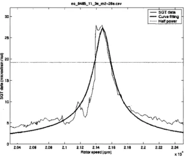
The results of the MATLAB® routine present the SGT data curve superimposed with the calculated SDOF analytical curve (Figure 6).

eo_B485_ 1 1_3e_m2:-2Se.clv

30

2.0<1 2.05 2.08 2.1 2.12 2.14 2.15 2.18 2.2 2.22 2.24 Rotortpeed(rpm) x ₁₀•

Figure 6 Curve fitting for damping extraction

The total damping value is given in the logarithmic decrement form. This method invokes that the forcing value throughout the resonance is constant (D parameter is constant). In reality, the force changes with regards to the engine rotating speed. Since the resonance band is very narrow (::::: 1000 RPM), the change in the forcing value is deemed negligible. The results are presented in section 7 .1.2.

3.3 Vibratory Stress Calculation

The experimental stress values are determined using the Hooke's Law:

{cr} = {E} { s} (3.3)

The deformation or strain (s) is obtained from the data reduction plots. Since it is assumed that the highest stress value will be at the surface of the turbine blade, only one strain gage (one direction) is necessary to determine the vibratory stress. The Y oung's modulus (E) is dependent on three parameters. The first parameter is the type of material used for the turbine blade since different materials have different Y oung's modulus. The second parameter is the metal temperature of the blade at the location of the strain gage

position. The Y oung's modulus decreases with the temperature elevation and therefore accurate temperature values are needed. The third parameter is the orientation of the strain gage. The materials used in a turbine blade are generally single crystal orthotropic materials. The orthotropic characteristic suggests that the Young's modulus of the material is not equal in all the axes of the crystal. Therefore, the orientation of the strain gage must be taken into account to determine the correct Y oung's modulus value. The results are presented in section 7.1.3.

FINITE ELEMENT MODEL BOUNDARY CONDITIONS DEFINITION

This subject will be concentrated on the application of boundary conditions using contact elements to determine the dynamic properties of a turbomachinery blade in an environment where the friction phenomenon is present. This study is performed using ANSYS® contact elements [18], which are meshed on the entire fixing area to simulate the interaction between the blade and the dise [16]. No assumptions were made initially for the blade-disc contact surface. The ANSYS® contact elements used require input for the static and dynamic friction coefficients and other parameters that have an effect on the convergence of the model. Before the modal analysis, a non-linear static analysis is performed with pre-stress effects, i.e. the blade metal temperature and the turbine shaft rotational speed. This static analysis, which is non-linear due to the addition of contact elements, calculates the new equilibrium position of the blade with respect to the dise due to the pre-stress effects. With the new equilibrium position found, a linear modal analysis is performed in order to obtain the natural frequencies and mode shape of the analyzed blade. The first four (4) natural frequencies and mode shapes are evaluated in this study. A convergence study is also performed to determine which contact element parameters have a significant influence on the natural frequencies values. The experimental results are extracted from strain gage tests for the natural frequencies and from a laser scan tests for the mode shapes. The analytical results are compared to the experimental results. Furthermore, experimental testing will be performed to determine the correct friction coefficient values as well as mode shape determination.

Contact elements are primarily used to simulate the contact stress and displacement between two moving components relative to each other. Current turbomachinery blade modal analyses are performed in PWC without the mating dise. The new method will

include part of the dise, and the contact elements will be used between the blade and the dise fixing.

4.1 Current Analysis

The current analysis omits the displacement between the blade and the dise and assumes no motion of the blade. The turbine blade is meshed using tetrahedral 1 0-node parabolic elements (SOLID92). These analyses typically have approximately 40,000 elements, 60,000 nodes and 180,000 degrees of freedom. The boundary conditions consist of zero displacement in the radial and tangential directions at the supposed contact line and zero displacement in the radial and axial direction for the front and rear fixing planes of the blade (Figure 7).

Radial and tangential displacements are blocked

Radial and axial displacements are

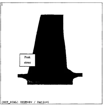
A static analysis is performed including pre-stress effects such as centrifugai force (rotation) and temperature. The static analysis determines a new mass [M] and rigidity [K] matrices due to the deformation of the blade. Once the static analysis is completed, a modal analysis is performed using the updated matrices. The results from this modal analysis are natural frequencies and mode shapes. Due to the total blockage contact line, there are peak stresses present in the fir-tree area, which do not reflect the reality (Figure 8).

(HCF_SCAL) USUM=Sv 1 Ratio=1

Figure 8 Blade stress with contact lines blocked

The unrealistic stress in the fir-tree area is the main reason for a more realistic modeling using contact elements. The vibratory stress can cause severe damage, which can extend up to the fracture of the blade, at the fir-tree area. Therefore, it is very important to be able to predict with more precision the stresses in that particular region.

4.2 New Analysis

The new analysis will be performed in much the same way, as is the current analysis (section 4.1). A static and modal analysis will be performed sequentially. The difference will be in the boundary conditions settings. In the new analysis, blockage of the blade will not be assumed. Contact elements will be used over the entire fir-tree area, and the static analysis will determine whether displacement occurs. To perform an ANSYS® three-dimensional static contact analysis, two types of elements must be used. The contact element (CONTA174) is used to represent the contact and sliding between the 3-D "target" surfaces and a deformable surface, defined by this element. CONTA174 is an 8-node element intended for general rigid-flexible and flexible-flexible contact analysis. The contact detection points are located either at the nodal points or at the Gauss points. The contact element is constrained against penetration into the target surface at its integration points. However, the target surface can penetrate through into the contact surface. The "target" surface is a geometrie entity in space that senses and responds when one or more contact elements move into a target surface. The target element (TARGE170) is used to represent various 3-D target surfaces associated with contact elements. The "contact-target" pair concept has been widely used in finite element simulations.

4.3 Meshing of Contact Elements

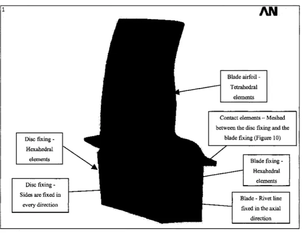
The meshing of the components is performed using CATIA ®. The section of the dise and the fir-tree region of the blade are meshed using 20-node hexahedral elements. Because of the complex shape of the blade's airfoil, 10-node tetrahedral elements are used for meshing (Figure 9). These analyses typically have approximately 80,000 elements, 100,000 nodes and 300,000 degrees of freedom. The boundary conditions used try to reflect the reality with more accuracy than the current analysis. The sides of the

dise portion are fixed in every direction while the blade is fixed in the axial direction using the nodes on the rivet ho le to simulate the use of the rivets.

1

Dise fixing -Hexahedral elements

Dise fixing -Sides are fixed in

every direction

Figure 9 Blade and dise meshing

AN

Blade airfoil -Tetrnhedral

elements

Contact elements - Meshed between the dise fixing and the

Blade fixing -Hexahedral

elements

Blade - Rivet line fixed in the axial

direction

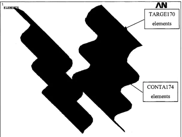
The meshing of the contact element pairs is performed using ANSYS®. Selections of nodes of the dise and blade fir-tree region in CATIA ® are created for meshing purposes in ANSYS®. The target elements (TARGE170) are meshed over the fir-tree area of the dise. There are no assumptions made with respect to the contact areas; and so the whole fir-tree is thus covered with the target elements. The same process is performed for the blade fir-tree region (Figure 1 0).

TARGE170 elements

CONTA174 elements

Figure 10 Contact elements mesh

Sin ce the part of the dise has been modeled, it is jugged flexible but no penetration can occur since "target" elements are used. The different contact types of the contact elements during the static and modal analyses are presented in the table below.

Table II

Contact type for the static and modal analyses

Contact Type Static Analysis Modal ~alysis ---~~-lnitially Touching

-l

Bonded Bonded Bonded Bonded Free ··-~-

~-~---1\b Separation 1\b Separation IFree

1\b Separatio~---1\b Separation

Rough _.

%ug~ =--=~~---

1\b Separation ___

Since a friction coefficient value is given to the contact elements, the "rough" contact type occurs during the static and modal analyses for this study. Therefore, after the static analysis is performed, only the elements that are touching to each other will be bonded while the contact elements pairs that are not touching will have no stiffness added.

4.4 Contact Element Input Data

The contact element pair has multiple parameters that have to be defined for the analysis to get a converged solution. The first parameter is the dynamic coefficient of friction (MU), which will have an effect on the limit shear stress and the relative sliding distance. The second and third parameters are the normal contact stiffness factor (FKN) and the penetration tolerance factor (FTOLN) respectively. These factors are related for the convergence purposes. The normal contact stiffness factor determines the penetration rigidity of the component while the tolerance factor determines whether the penetration compatibility is satisfied when using the penalty and Lagrange method. The contact compatibility is satisfied if the penetration is within a tolerance of the FTOLN value multiplied by the depth of the underlying solid. Therefore, if the FKN and the FTOLN factors are too low, the analysis will not converge due to the presence of a higher than allowed level of penetration. The fourth and fifth parameters are required for a smooth transition zone between static and dynamic friction given by the following equation [4.1]:

JL =MU x

(1

V,.e!)

JL is the static coefficient of friction, MU is the dynamic coefficient of friction presented previously. The parameters FACT for the ratio between the static and dynamic friction coefficients and DC for the decay coefficient are required. Vret is the slip rate between the blade and the fixing calculated at each time step by ANSYS®. Since these parameters are not known, a convergence study has been performed and will be presented in the following chapter on these five parameters. The contact element pair

has many other parameters but they were kept at their default values since they had no effect on frequency values and mode shapes. The results are presented in section 7 .2.

EXPERIMENTAL TESTING

Experimental datais extensive at PWC. For certification purposes, ali HP or CT blades have a strain gage test (SGT) performed to determine the resonances in the running range and the vibratory stress associated with them. A strain gage test is done in test cell using a real engine as a test vehicle. Strain gage are attached to any components as required by the engineer. When the engine is running, a data acquisition system records the strain gage signal as well as the engine rotating speed. A Fast Fourier Transform is performed by the data acquisition system on the strain gage recorded time signal. This step transforms the time signal into the frequency domain and using the rotating speed, a waterfall plot is generated. For a turbine blade certification, these tests require the application of strain gages on different blades, the gages being located on high strain areas based on the FEM model. Therefore, the accuracy of the mode shape is of prime importance in order to assess the HCF life of the component. Due to highly complex and expensive method of performing these strain gage tests, a static test at normal temperature is developed to further study the contact elements as boundary condition in the blade FEM model. The main goal of the experimental testing is to determine the friction coefficient for the model in order to reproduce the mode shapes at the correct natural frequency values. Furthermore, the need for a specifie friction coefficient for every mode shape might arise. In addition, contact testing using chalk between the blade and dise contact faces will be applied and the results will be correlated with the FEM modelling.

5.1 Experimental Test Model

To perform the experimental testing, a blade and dise will be used. To correlate the results of the experimental testing on the FEM results, the boundary conditions have to be the same. For the experimental test, the blade will be assembled on the dise. The dise

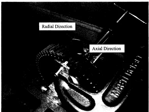
will be held in a specially designed fixture to avoid any resonance in the frequency range of interest. To simulate centrifugai force (CF) loading, two screws are forced inside the chamfer of the rivet hole, which will create an upward force due to its conical shape (Figure 11). Refer to Figure 12 for illustration of the conical shape ofthe rivet hole.

Figure 11 Experimental test mount simulation of centrifugai force

To recreate the same boundary conditions in the FEM model, the centrifugai force was removed and replaced by a displacement ofO.l inch (approximate value) in the axial and radial directions based on the conical shape at which the screws are inserted (Figure 12).

Figure 12 FEM model experimental boundary conditions

5.2 Response Signature Recording

When performing modal testing, usually a hammer is used to excite the component while an accelerometer is used to register the response signal of the component. This is not a concem when the component weighs significantly more than the accelerometer. In this case, the weight on the CT blade is less than ten (1 0) times the weight of the smallest accelerometer. Therefore, to avoid the shift in :frequency due to weight of the accelerometer, a PolyTec laser vibrometer will be used instead (Figure 13).

Figure 13 PolyTec Laser Vibrometer

The laser vibrometer will record nine (9) different points of the blade's airfoil so that a mode shape can be created using ali the signais (Figure 14).

~

•

---•

• • •

• - •