INTERACTIVE SEARCH FOR COMPROMISE SOLUTIONS IN MULTICRITERIA
GRAPH PROBLEMS Lucie Galand
LIP6, University of Paris 6, France
Abstract: In this paper, the purpose is to adapt classical interactive methods to multicriteria combinatorial problems in order to explore the non-dominated solutions set. We propose an interactive procedure alternating a calculation stage determining the current best compromise solution and a dialogue stage allowing decision maker to specify his/her preferences. For the calculation stage, we propose an efficient procedure which relies on algorithms providing k-best solutions of a scalarized version of the problem. Moreover, we show how to exploit previous iterations to speed-up the interactive process. We provide numerical experiments of our method on multicriteria shortest path and spanning tree problems. Keywords: Multiobjective optimisations, interactive approaches, decision making, graphs, path planning, trees.
1. INTRODUCTION
Traditionally, graph problems are considered in the framework of the single objective optimiza-tion. However, in many practical situations, the value of a solution must be assessed with respect to several criteria. For example, in a path problem, the choice of the most satisfactory route can be de-termined including multiple aspects like cost, dis-tance, time and accessibility. Generally, there is no unique optimal solution in a multicriteria problem but rather a set of non-dominated solutions (i.e., solutions such that there does not exist another better feasible solution with respect to all criteria) among which the decision maker (DM) selects its favorite (i.e., the one representing the best com-promise for him/her). However, due to the poten-tially large size of this set in practice, its complete generation can be very hard. Moreover it is often difficult for a DM to select a preferred solution among a high number of alternatives. To overcome these drawbacks we use an interactive method to explore the set of non-dominated solutions accord-ing to the DM’s preferences. There are two types
of approaches for interactive procedures in multi-criteria combinatorial optimization. The first one consists of two phases: a prior generation of the whole non-dominated solutions set (or an approx-imation of this set) and an interactive exploration of this set in order to find the best compromise solution for the DM. This type of procedure is proposed in (Gabrel and Vanderpooten, 2002) for example, to select efficient paths in a multiple criteria graph problem to be solved for scheduling an earth observing satellite. This approach allows to get all non-dominated solutions and thus all potentially best compromise solutions. It is appro-priate when the size of the graph is reasonable and when we have no information about a priori DM’s preferences since we can efficiently explore the whole non-dominated solutions set. Nevertheless the duration of the first phase can be very long. Indeed there are instances for which the number of non-dominated solutions is exponential in the size of the instance, see (Hansen, 1980) for the multicriteria shortest path problem (MSPP) and (Hamacher and Ruhe, 1994) for the multicriteria
spanning tree problem (MSTP). The second in-teractive approach directly determines a first best compromise solution without any prior generation of the non-dominated solutions set. Then during the exploration stage, the DM can specify his/her preferences in relation to the proposed solution and the notion of best compromise is updated. A new calculation stage is then performed to search a better solution for the DM. This type of procedure is proposed for MSPP in (Granat and Guerriero, 2003) for example.
Since the first approach requires a pre-process which is sometimes very long, we focus here on the second interactive approach. The main difficulty of this approach is to determine efficiently the best compromise solution among a combinatorial set. The method we propose efficiently provides the DM’s favorite solution by an interactive process without necessarily compute the entire set of non-dominated solutions. Several efficient interactive methods are proposed for the bicriteria short-est path problem (see for example (Rodrigues et al., 1999; Murthy and Olson, 1994)) but our method neither depends on the problem nor on the number of criteria.
In Section 2 we first recall notion of best com-promise and discuss about the complexity of this problem, then we propose an efficient algorithm to determine the best compromise solution of a multicriteria graph problem (MSPP and MSTP in particular). We present some numerical exper-iments obtained on MSPP and MSTP. In Section 3, we explain how this algorithm is integrated into our interactive method and how the previous iterations can be used to speed-up the search of the best solution during interactions.
2. GENERATING A BEST COMPROMISE SOLUTION
2.1 Notations
Let G = (V, E) be a graph (directed or not, according to the considered problem) where V = {1, . . . , n} is a finite set of nodes and E ⊆ V × V is a finite set of edges (or arcs). With any edge (or arc) u ∈ E, is associated a q-dimensional vector of criteria c(u) = (c1(u), . . . , cq(u)) with c(u) ∈ Nq.
In this article we consider both MSPP and MSTP. A feasible path of MSPP is a sequence of nodes beginning by an origin node and ending by a destination node, such that two nodes v and v′
can follow in the sequence if there exists an arc (v, v′) ∈ E. A feasible tree of MSTP is a set
of |V | − 1 edges of E without cycle. We call S the set of arcs forming a path in MSPP or the set of edges forming a spanning tree in MSTP. S is evaluated by the q-dimensional vector of criteria c(S) = (Pu∈Sc1(u), . . . ,Pu∈Scq(u)). A
solution of a problem PG is a q-dimensional
vec-tor x = (x1, . . . , xq) with x ∈ Nq such that there
exists in G a path or a spanning tree S such that c(S) = (x1, . . . , xq). Let X be the set of
feasible solutions (i.e., the set of q-dimensional vectors corresponding to the evaluation of a pos-sible path or pospos-sible spanning tree in G), and let N D be the set of non-dominated solutions (i.e., N D = {x ∈ X, ∄y ∈ X, ∀i ∈ Q yi ≤ xi and
∃i ∈ Q, yi< xi} with Q = {1, . . . , q}). Since the
problem of minimizing a q-dimensional vector is ill-defined, we use a scalarizing function f to value a q-dimensional vector in a unique cost. The best solution according to f is the best compromise solution. Based on these definitions and notations, the multicriteria optimization graph problem is:
(PG): minx∈Xf (x)
In the next subsection, we define the function f representing the notion of compromise.
2.2 Best compromise solution
If f is defined as a weighted sum of criteria like ∀x ∈ X, f1
ω(x) =
Pq i=1ωixi
where ωi is the weight assigned to criterion i, the
problem (PG) is easy to solve. Indeed, in this case
f1 ω(x) =
Pq
i=1ωici(S) =P q
i=1ωiPu∈Sci(u)
i.e., f1 ω(x) = P u∈S Pq i=1ωici(u) = c1ω(S) with ∀u ∈ E, c1 ω(u) = Pq i=1ωici(u).
Thus, to find the minimal solution according to f1
ω when G is valued by the q-dimensional
vec-tor of criteria c, we just have to search for the minimum solution (shortest path or minimum spanning tree) when G is scalarized by c1
ω. Hence
we get a classical monocriterion problem which can be solved in polynomial time. However linear functions are not really satisfactory to determine compromised solutions because they allow full compensations between good and bad values of criteria. Moreover, it is well known in multicriteria optimization that as soon as X is not convex, opti-mizing a linear function does not enable to obtain “unsupported” solutions (i.e., solutions that do not belong to the boundary of the convex hull of X). This eliminates an a priori good compromise as we can see with Example 1.
Example 1. Let a path problem where cost and time are considered. Suppose there exists three routes corresponding to the non-dominated so-lutions x = (100, 120), y = (45, 180) and z = (0, 240) (where the first and the second val-uation represent respectively the cost and the time of the route). Solution y represents the best compromise. We then determine for which vector
ω = (ω1, ω2), y minimizes fω1. We have:
fω1(x) = 100ω1 + 120ω2, fω1(y) = 40ω1+ 190ω2
and fω1(z) = 240ω2.
fω1(y) < fω1(z) if ω1 < 98ω2 but when ω1 < 76ω2,
f1
ω(x) < fω1(y) and then x minimizes fω1. Then
whatever ω ∈ R2, y never minimizes f1
ω while it
represents the best compromise.
Through this example, we see that the weighted sum is not a satisfactory way to define the notion of compromise. Thus we use another type of func-tion measuring the distance to a reference point in the sense of the Tchebycheff weighted norm (i.e. the infinity norm (Wierzbicki, 1986)). Indeed, this function is often used in interactive proce-dures (Steuer and Choo, 1983; Vanderpooten and Vincke, 1989), because it allows to explore the whole set of non-dominated solutions (supported or unsupported) by varying the weighting vector. We use the classical scalarizing function f∞
ω as the
distance to a reference point r: f∞
ω (x) = maxi∈Qωi|xi− ri|
The problem we address now is the best compro-mise search according to the Tchebycheff weighted norm:
(Pω): minx∈Xfω∞(x)
In this section the notion of compromise is based on the classical ideal (I) and nadir (N ) points, as reference points, which allow to border the non-dominated solutions set:
∀i ∈ Q, ri= Ii and ωi=|Ni1−Ii| with:
Ii= minx∈N Dxi and Ni= maxx∈N Dxi (1)
We will see in Section 3 that I and N (and thus r and ω) can be modified in an interactive process to adapt the notion of compromise to the DM’s preferences.
2.3 Complexity of the best compromise search It is shown that
(M inM ax): min
x∈Xmaxi∈Q
X
(u,v)∈S
ci(u, v)
is a NP-Hard problem for MSPP (Yu and Yang, 1998) and for MSTP (Hamacher and Ruhe, 1994). Since (M inM ax) reduces to (Pω) with
ω = (1, . . . , 1) and I = (0, . . . , 0), (Pω) is also a
NP-hard problem.
2.4 Optimality principle
Searching for a best compromise solution (i.e., for the optimal solution of (Pω)) rather than a set
of non-dominated solutions is more discriminat-ing and then should improve the search. But in addition to the NP-hardness of (Pω), it presents
another difficulty: the optimality principle does not hold, as we can see for MSPP in Example 2. Example 2. Figure 2 represents bicriteria graph proposed by (Hansen, 1980). One best
compro-(0, 2) (0, 0) (2, 0) 1 3 5 2 4 (4, 0) (0, 0) (0, 0) 6 7 (0, 4) (1, 0) (0, 1)
Fig. 1. Instance proposed by (Hansen, 1980) mise path in this graph is the path P1= h1, 3, 5, 6, 7i
corresponding to the solution x1 = (4, 3). But
the sub-path h1, 3, 5i valued by (0, 3), is the worst compromise among all paths from vertex 1 to ver-tex 5. The path h1, 2, 3, 5i for example, valued by (1, 2) represents a better compromise than (0, 3).
We see through this example, that with f∞ ω , a
sub-path from an optimal path is not necessarily optimal. It even can be the worst sub-path. Then using a constructive approach based on optimal sub-paths, like dynamic programming, seems to be unappropriate to determine the best compro-mise path.
Figure 2 illustrates a bicriteria instance for which we can come to the same conclusions for MSTP. Indeed, on this instance, the best compromise spanning tree, formed by the edges (a, b) and (b, c) is valued by (2, 2) which does not include the best compromise edge (a, c) valued by (1, 1).
(0,2) (2,0) c a (1,1) b Fig. 2. An instance of MSTP
We now present our approach determining the optimal solution of (Pω) without using the
opti-mality principle.
2.5 Calculation algorithm
We saw above that minimizing f1
ω enables to
handle in polynomial time scalarized problems. But it doesn’t allow to find the best compromise solution. However, the minimizing f∞
ω solution
often achieves a good performance according to f1
ω, even it is not the best. Therefore, we propose
to enumerate solutions in increasing order of f1 ω.
We can then reach all feasible solutions by using a scalarized version of the graph. In this respect,
we establish a property stopping the enumeration as soon as we can ensure to have generated the optimal solution of (Pω).
For all x ∈ X ⊂ Nq let vector ¯x
ω of Nq defined as ∀i ∈ Q, ¯xωi = Ii+ 1 ωif ∞ ω (x) then we have: Property 1. ∀x ∈ X, ∀y ∈ X, f1 ω(y) > fω1(¯xω) =⇒ fω∞(x) < fω∞(y)
Proof 1. Let y, x ∈ X, such that f1
ω(y) > fω1(¯xω) thusPqi=1ωiyi>P q i=1ωiIi+P q i=1fω∞(x)
i.e.,Pqi=1ωi(yi− Ii) > qfω∞(x) and then,
Pq
i=1ωi(|yi− Ii|) > qfω∞(x) (2)
Moreover since f∞
ω (y) = maxi∈Q(ωi|yi− Ii|),
Pq
i=1fω∞(y) ≥
Pq
i=1ωi|yi− Ii| hence, from (2)
we have qf∞ ω (y) = Pq i=1fω∞(y) > qfω∞(x) i.e., f∞ ω (y) > fω∞(x) 2
Thus, for any solution z ∈ X such that f1 ω(z) >
f1
ω(y) (with fω1(y) > fω1(¯xω)), we have fω∞(z) >
f∞
ω (x). There is no solution following y in the
increasing order of f1
ω enumeration which can be
better than x in sense of f∞
ω . During the
enumer-ation, once solution y is generated, the current optimal solution x (minimizing f∞
ω ) is the optimal
solution of (Pω). Using this property, the
algo-rithm presented in Figure 3 generates solutions in increasing order of f1
ωthanks to k-best algorithms
((Jim´enez and Marzal, 2003) for the path problem and (Katoh et al., 1981) for the spanning tree problem). This enumeration is stopped when a solution y such that f1
ω(y) > fω1(¯xω) is
gener-ated. The same type of approach is proposed in (Paixao et al., 2003) to optimize another non-linear function (Minimum-cost norm). But this norm does not allow to reach all non-dominated solutions (Wierzbicki, 1986). Figure 4 illustrates Determine ideal point I and nadir point N x1←− argmin x∈Xfω1(x), s∗←− fω∞(x1) B ←− f1 ω(¯xω), x∗←− x1, k ←− 2 Whilef1 ω(xk−1) ≤ B
Generate the kth best solution xk according to f1 ω
Ifthere is no more solutions Then exit from the while
Iff∞
ω (xk) < fω∞(x∗) Then
B ←− f1
ω(¯xkω), x∗←− xk
k ←− k + 1
Return: x∗, optimal solution for f∞ ω
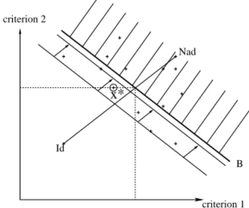
Fig. 3. Generation of the best compromise solution the algorithm idea on a bicriteria problem. In this figure, arrows indicate the direction of the search according to f1
ω. The surrounded solution
is the optimal solution x∗. The bolded straight line
represents the hyperplan beyond which solutions are worst than x∗ according to f∞
ω . This straight
line corresponds to the value B in the algorithm
on Figure 3. Solutions in the hatched zone will then never be generated.
x* criterion 2 criterion 1 Nad B Id
Fig. 4. Algorithm sequencing
2.6 Results
Some numerical experiments have been done on this algorithm for MSPP and MSTP. Table 1 summarizes results obtained for several instances. Tests were executed on a Pentium IV with 2.5GHz processor. The algorithm was implemented in C++. For MSPP, the number of arcs and their costs vector are randomly generated. For MSTP, tests are executed with complete graphs where the costs vector of any edge is randomly determined.
Table 1. Experimental results
Multicriteria shortest path problem (ms)
# nodes 100 200 500 800 1000 # arcs 470 7 543 46,975 120,192 187,615 5 criteria 0.9 4 25 66 94 10 criteria 4 16 73 167 205 20 criteria 18 55 146 362 620 # nodes 1500 2000 2500 3000 # arcs 422,056 750,248 1,172,301 1,689,311 5 criteria 233 467 771 1.15s 10 criteria 350 676 1s 1.6s 20 criteria 1.33s 3.12s 4.3s 6s
Multicriteria spanning tree problem (ms)
# nodes 5 8 10 12 15
5 criteria 0 3 20 125 1.33s
10 criteria 0 35 964 10.6s
-20 criteria 0 99 9.9s -
-These tables show that our algorithm is very ef-ficient for MSPP. Indeed, solutions are quickly found even when graphs have many nodes and arcs. However for MSTP, our algorithm is only ef-ficient for graphs having at most 15 nodes. In this table, ”-” means that execution time is greater than 20 minutes. Nowadays, to our knowledge, there is no algorithm which determines the best compromise spanning tree significantly faster. The results obtained for this problem seem to be quite satisfactory.
These results show we can efficiently generate a best compromise solution, and then it seems
interesting to integrate this algorithm into an in-teractive procedure by using the second approach introduced in Section 1.
3. INTERACTIVE PROCEDURE 3.1 Interactive process
In the previous section we presented an algorithm finding efficiently the best compromise solution of (Pω) defined by the ideal and nadir points. But
on the one hand, notion of compromise depends on DM’s preferences (a favorite solution for one DM has no reason to be the favorite for another DM). On the other hand, DM’s preferences (a priori or not) can evolve during the search when he/she realizes what kind of performance and compromise can be obtained. That is why, it seems relevant resorting to an interactive procedure to adapt the notion of compromise. As we said ear-lier, the interactive procedure determines first the best compromise by using the algorithm presented in Section 2. The solution is then proposed to the DM. He/she can specify on which criterion he/she is not satisfactory, or stop the process if the current solution suits him/her. His/her pref-erences specifications modify ω and r by changing I and N in order to direct the search for his/her preferred solutions (at the first step, ideal and nadir points are defined by (1)). In the interactive procedure we propose, the DM can specify his/her preferences in three manners:
• improving criterion performance
• setting an aspiration level for a criterion (i.e. an ideal performance)
• setting a reservation level for a criterion (i.e. a maximal admissible performance)
These specifications either modify the ideal or the nadir point and therefore vectors ω and r to adapt the notion of compromise to the DM’s preferences. To improve the performance of a criterion i, we set Ni to the value of the ith criterion of the current
solution. To set an aspiration level, we modify the ideal point value for the considered criterion. We modify the criterion performance of nadir point to set the reservation level.
3.2 Use of previous iterations
The time required to find the current best com-promise solution depends on the complexity of k-best algorithms (algorithm in (Jim´enez and Marzal, 2003) determines k shortest paths in O(m + nlogn + klogk) and the one in (Katoh et al., 1981) determines k best spanning trees in O(km + min(n2, m log log n)) where m = |E| et
n = |V |). Thus it can be interesting to avoid
the systematical execution of the algorithm after a dialogue with the DM in order to reduce the running time of the whole interactive process. In this perspective we establish the following prop-erty using information from the previous iteration. To simplify notations fh(x) denotes fω(x) at
iter-ation h and ¯zh= Ihi+ 1
ωhifh∞(z).
Property 2. Let Zh be the set of solutions
gener-ated at iteration h and t ∈ Zhbe the last solution
generated at iteration h (f1
h(t) = maxx∈Zhf 1 h(x)).
Let z = arg minx∈Zhf ∞
h+1(x). Then:
f1
h(¯zh+1) < fh1(t) =⇒ z = arg minx∈Xfh+1∞ (x)
Proof 2. Let y ∈ X such that y /∈ Zh and
f∞ h+1(y) ≤ fh+1∞ (z). y /∈ Zh=⇒ fh1(y) ≥ fh1(t) but f1 h(t) > fh1(¯zh+1) thus fh1(y) > fh1(¯zh+1) i.e., f1 h(y) > Pq i=1ωhiIh+1i+ Pq i=1 ωhi ωh+1if ∞ h+1(z) by hypothesis, f∞ h+1(y) ≤ fh+1∞ (z) and f∞
h+1(y) = maxiωh+1i(|yi− Ih+1i|) thus ∀i ∈ Q,
fh+1∞ (y) ≥ ωh+1i(|yi− Ih+1i|) ≥ ωh+1i(yi− Ih+1i) then fh1(y) > Pq i=1ωhiIh+1i + Pq i=1ωhi(yi − Ih+1i) i.e., f1 h(y) > f 1
h(y) which is impossible.
Solution y ∈ X such that y /∈ Zh and fh+1∞ (y) ≤
f∞
h+1(z) when fh1(¯zh+1) < fh1(t) can’t exist. 2
Hence, if f1
h(¯zh+1) < fh1(t), then the algorithm
does not need to be executed at iteration h + 1 to compute the best solution, because we know it is z. Besides, during a calculation stage at itera-tion h, several soluitera-tions are generated. When the calculation is restarted at iteration h + 1 (after a dialogue with the DM) many solutions generated at iteration h are re-generated. In order to avoid generation of the same solution several times, we propose to search for the best compromise accord-ing to f∞
h by using ω1as the direction researching
for all iterations h. Thus, when the algorithm is executed, it runs from the last solution generated at the last iteration. Hence, we generate a solution only one time during the whole process. Note that property 2 still holds since by changing f1
h in f11
in the proof we come to the same conclusions. Example 3 illustrates how our algorithm runs on three iterations.
Example 3. We consider an instance of MSPP represented in Figure 5. On this graph, each arc u is valued by the vector c(u) and the number c1(u)
which corresponds to the scalarized version of the problem. We search for the best path from node a to node g. Ideal and nadir points are determined: I = (8, 11) and N = (18, 19). Thus we have ω = (1
10, 1 8).
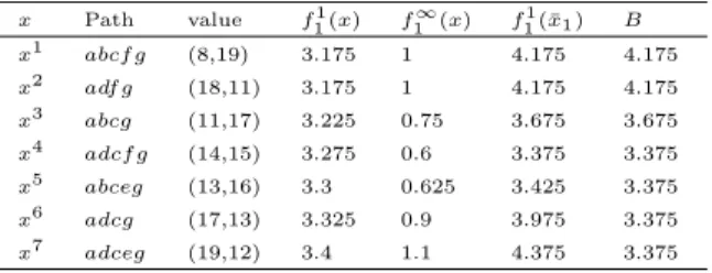
Then we settle scalarized graph (scalar valuation of each arc in Figure 5). At the first iteration, 7 solutions are generated. They are given in the Table 2 in their generation order. As f1
a
b
c
d
(6,3)g
f
e
(1,4) 0.944 (4,4) (2,4) 0.722 1.917 0.694 (7,6) (2,4) (10,4) (2,3) 0.597 (5,3) 0.931 0.847 (2,5) (6,10) 0.972 (2,6) 0.975 1.611 0.722 (4,2) 1.45 0.6Fig. 5. bicriteria graph and corresponding scalar-ized version
Table 2. Ordered generation of solutions x Path value f1 1(x) f ∞ 1 (x) f 1 1(¯x1) B x1 abcf g (8,19) 3.175 1 4.175 4.175 x2 adf g (18,11) 3.175 1 4.175 4.175 x3 abcg (11,17) 3.225 0.75 3.675 3.675 x4 adcf g (14,15) 3.275 0.6 3.375 3.375 x5 abceg (13,16) 3.3 0.625 3.425 3.375 x6 adcg (17,13) 3.325 0.9 3.975 3.375 x7 adceg (19,12) 3.4 1.1 4.375 3.375
the algorithm can then stop. The best compromise is solution x4 = (14, 15), corresponding to the
path adcf g. This solution is thus proposed to the DM. Suppose he/she wants to improve the first criterion performance. He/she then specifies an aspiration level for this criterion and ideal point is updated to (7, 11). f1
1(x7) = 3.4 and f11(¯x52) =
3.388 (where f∞
2 (x5) = mini=1,...,7f2∞(xi)). Thus
property 2 holds here. The solution x5 = (13, 16)
corresponding to the path abceg is thus pre-sented to the DM as a new compromise solution. f∞
2 (x5) < f2∞(x4) which corresponds to the
de-sired performance. Suppose now he/she specifies a reservation level for the second criterion to 14. The nadir point value is then updated to (18, 14). Property 2 doesn’t hold at this iteration, thus the algorithm continues its enumeration of solu-tions. Solution x8= (12, 18) corresponding to the
path abeg is generated. f1
1(x8) = 3.45 which is
greater than f1
1(¯x63) = 3.416 (where f3∞(x6) =
mini=1,...,7f3∞(xi)). The algorithm can stop. x6is
the best solution at iteration 3.
4. CONCLUSION
We propose in this article an algorithm which determines efficiently, in the majority of cases, the desired compromise solution, avoiding generation of all non-dominated solutions. We integrate this algorithm in an interactive procedure to take into account the possible evolution of the DM’s prefer-ences during the exploration. We use the previous iterations of the interactive procedure in order to speed-up the search of the DM’s favorite solution. The main advantage of our approach is its porta-bility. Indeed it can be applied to all types of com-binatorial multicriteria problems for which there
exists an efficient k-best solutions algorithm. The algorithm can then be integrated into an efficient interactive procedure.
REFERENCES
Gabrel, V. and D. Vanderpooten (2002). Enu-meration and interactive selection of efficient paths in a multiple criteria graph for schedul-ing an earth observschedul-ing satellite. European Journal of Operational Research 139, 533– 542.
Granat, J. and F. Guerriero (2003). The inter-active analysis of the multicriteria shortest path problem by the reference point method. European Journal of Operational Research 151, 103–118.
Hamacher, H.W. and G. Ruhe (1994). On span-ning tree problems with multiple objectives. Annals of Operations Research 52, 209–230. Hansen, P. (1980). Bicriterion path problems. In:
Multiple Criteria Decision Making: Theory and Applications, LNEMS 177 (G. Fandel and T. Gal, Eds.). pp. 109–127. Springer-Verlag, Berlin.
Jim´enez, V. M. and A. Marzal (2003). A lazy ver-sion of eppstein’s k shortest paths algorithm. In: WEA. pp. 179–190.
Katoh, N., T. Ibaraki and H. Mine (1981). An algorithm for finding k minimum spanning trees. SIAM J. Computing 10(2), 247–255. Murthy, I. and D.L. Olson (1994). An interactive
procedure using domination cones for bicrite-rion shortest path problems. European Jour-nal of OperatioJour-nal Research 72, 417–431. Paixao, J.M.P., A.Q.V Martins, M.S. Rosa and
J.L.E. Santos (2003). The determination of the path with minimum-cost norm value. Net-works 41(4), 184–196.
Rodrigues, J.C., J.C.N. Cl´ımaco and J.R. Cur-rent (1999). An interactive bi-objective short-est path approach: Searching for unsupported nondominated solutions. Computers & Oper-ations Research 26, 789–798.
Steuer, R.E. and E.-U. Choo (1983). An interac-tive weighted Tchebycheff procedure for mul-tiple objective programming. Mathematical Programming 26, 326–344.
Vanderpooten, D. and Ph. Vincke (1989). Descrip-tion and analysis of some representative inter-active multicriteria procedures. Mathematical and Computer Modelling 12(10/11), 1221– 1238.
Wierzbicki, A.P. (1986). On the completeness and constructiveness of parametric characteriza-tions to vector optimization problems. OR Spektrum 8, 73–87.
Yu, G. and J. Yang (1998). On the robust shortest path problem. Comput. Oper. Res. 25(6), 457–468.