Stockholding: Does housing wealth matter?
L. Arrondel, F. Savignac
yzSeptember 2009 (preliminary version)
Abstract
Following recent developments in the literature about portfolio choices (Flavin and Yamashita, 2002; Cocco, 2004; Yao and Zhang, 2005), this paper analyses the empirical link between stockholding and housing wealth. We use the French wealth survey (Enquête Patrimoine2004, Insee) that give us detailed informa-tion on households portfolio composiinforma-tion (housing and …nancial wealth, mort-gages), socio-demographic variables, and several measures of attitudes (risk aversion, scales on time preference) and exposition to various risks (income, unemployment, health, business). We …nd that housing wealth crowds out stock market participation: a homeowner who moves from the …rst decile of the distribution of the housing wealth to the last one increases his probability to own stocks from 0.18 to 0.37. Among the other signi…cant determinants of the equity premium puzzle, we emphasize the role of transaction and information costs, the attitude toward risk and the exposition to various risks in hampering investments in stocks.
Keywords: Portfolio choice, housing demand, life-cycle model
JEL classi…cation: D91, G11, R22, E21
CNRS-PSE, Banque de France. Paris-Jourdan Sciences Economiques Ecole normale supérieure 48 bd Jourdan - 75014 Paris. E.mail: [email protected]
yBanque de France. 31 rue croix des petits champs 75001 Paris E.mail:
zThis paper represents the views of the authors and should not be interpreted as re‡ecting those
1
Introduction
The recent …nancial crisis sheds light on the interaction between indebtedness, housing wealth and …nancial portfolio for households. In France, the housing price index and the stock price index decreases respectively by 7% and 40% between March 2008 and March 2009. At the same time, households’overindebtedness increases a lot (+16% between January 2009 and March 20091). All these changes impact dramatically
households’wealth in all of its dimensions.
In this paper, we focus on the link between risky portfolio and the households’ real estate exposure to risk. As this asset is the main component of households’worth and often acquired by highly leveraging, it creates a risk that is taken into account by households when deciding the composition of their …nancial portfolio. Moreover, housing wealth is also a speci…c asset due to its illiquid nature that may constrained households’decision to rebalance their portfolio.
An additional motivation for this paper is to contribute to the empirical literature about the equity premium puzzle. Indeed, the standard life cycle framework predicts that households’ wealth is fully diversi…ed and does not vary during the life cycle (Merton, 1971). In particular, the share of risky assets in total assets is always positive and depends on assets features (risk and return) and on the relative risk aversion of stockholders but it does not vary according to other stockholders’ characteristics such as their age. However, a large strand of the empirical literature emphasizes the existence of an equity premium puzzle: one observes a low risky assets holding that the standard life cycle model is not able to explain, except if eccentric values of risk aversion are considered. This equity premium puzzle deals both with the amount of risky assets and with the participation of households to …nancial markets (Haliassos, 2003). For example, only 20% of French households own …nancial risky assets directly or indirectly via mutual funds (the proportion of households participating directly to the stock market is more limited (15%)).
Various modi…cations of the standard hypothesis of the life cycle model are pro-posed in the literature to account for the equity premium puzzle. It may be due to transaction costs (King and Leape, 1998), credit constraints (Gollier, 2001) or the existence of other risks (Kimball, 1993). In this last case, unavoidable risks such as unemployment risk or uncertainty about future incomes lead households to moderate their global exposure to risk by reducing their holding of stocks. This behaviour, called temperance, may thus explained the equity premium puzzle. Recently, the e¤ect of background risks was generalized by taking into account the risk induced by real estate exposure (Fratantoni (2001), Flavin and Yamashita (2002), Cocco (2004), Yao and Zhang (2005)). These papers show that housing wealth crowds out stock-holding due to liquidity constraints and to the risk associated with owning real estate. They also …nd that the heterogeneity over the life cycle observed in households’port-folio composition (in particular, the increase in stockholding with age) may be due
1Source: Banque de France, Secretariat of the Household Debt Commissions.
to changes in housing wealth. Young households invest in housing by getting mort-gages. They take into account the risk associated with this debt when determining their stockholding. In other words, the risk associated with indebtedness lead them to limit their participation to (risky) …nancial markets. Afterwards, the reimbursement of the contracted debt reduces the share of housing wealth in the total net wealth as well as the risk associated with the global portfolio (…nancial and housing wealth). Households become thus interested in increasing their risky …nancial wealth in order to bene…t from higher returns.
In addition, other empirical studies (Yamashita, 2003; Saarimaa, 2008) …nd a neg-ative correlation between stockholding and housing wealth with respectively US and Finnish data. Here, we estimate a similar model on French wealth data. Compared to the previous papers cited above, our empirical analysis fully takes into account the risk aversion of the households as well as other background risks (income risk, unem-ployment risk) that were previously studied separately from the real estate exposure to risk (for instance, see Guiso et al. (1996)).
The paper is organized as follows. Recent developments of the literature about portfolio choice, especially about the role of housing, are summarized in the second section. Then, our dataset as well as a …rst descriptive analysis of households port-folio is presented before estimating the relationship between households’risky asset demand and di¤erent sources of background risks.
2
Recent Developments in Portfolio Choice
In this section we …rst emphasize recent developments on intertemporal portfolio choice mainly concerning the e¤ect of age, transactions costs, and uncertainty re-garding future income on risky asset demand. Then we investigate how housing could be introduced in this model.
2.1
Complete Markets
Optimal portfolio theory, as developed by Arrow (1965), describes an investor who maximizes, at a given period, utility, u(:); by allocating wealth, W , over the di¤erent assets available on the market. If shares are divisible and capital markets are perfect, and if the investor’s relative risk aversion ( u00W=u0) is constant, the proportion of
wealth devoted to each share, w is independent of W . In addition, the demand for risky assets is a positive function of W if absolute risk aversion ( u00=u0) is falling in
wealth.
This theory can be combined with a life-cycle model, in which the agent chooses both the optimal level of consumption and portfolio allocation each period (Merton, 1969 and 1971, and Samuelson, 1969). Markets are still considered to be complete (no future income risk) and perfect (no transaction costs). If utility is additively separable over time, and if the distribution of share prices is described by geometric
Brownian motion, then portfolio structure is independent of age (the hypothesis of rational myopia2) and of consumption choices. In addition, investors hold all shares
available on the market (risk free as well a risky shares) in some proportion (two funds separation theorem): in other words, portfolios are complete.
Gollier and Zeckhauser (2002) try to explain changes in portfolio composition over the life cycle. They show that if investors’ absolute tolerance for risk ( u0=u00, the
inverse of absolute risk aversion) is convex (and not linear, as in Merton’s model) the young will invest more in risky assets than will the old.3
Other recent extensions have considered agents’behavior in incomplete and imper-fect markets. These models try to explain the limited diversi…cation of households’ portfolios, and in particular the limited participation of agents in the market for …nancial risky assets (the equity premium puzzle).4
2.2
Imperfect and Incomplete Markets
Holding and transaction costs are the only viable explanation of incomplete portfolios, notably with respect to shares (Haliassos, 2003).5 King and Leape (1987 and 1998),
for example, generate incomplete portfolios by introducing …xed transaction costs and costs of information acquisition (in terms of both time and money) into Merton’s model. In particular, investment in risky assets, which is associated with both more information and higher transaction costs, rises with global wealth, which allows such costs to be borne, and with age and education, both of which measure the agent’s information stock.
Recent work has also considered the management of multiple risks by savers. Portfolio choice is then analyzed in the presence of exogenous risks against which no insurance is available (background risk). The e¤ect of multiple sources of risk on savers’ behavior, particularly on their demand for risky assets, will depend on both the type of risk and individuals’ preferences. Pratt and Zeckhauser (1987), Kimball (1993), and Gollier and Pratt (1996) have shown under which conditions on preferences there is substitution between endogenous portfolio risk and independent exogenous risk, such that individuals reduce their demand for risky assets as other risks appear (with respect to income, health of the household etc.)
Pratt and Zeckhauser (1987) show that the presence of undesirable background
2Apart from assets’ technical characteristics (return and risk), this myopia is linked to agents’
tolerance for risk (the inverse of their risk aversion) which has to be linear in wealth (Mossin, 1968).
3The demand for risky assets is related in a convex manner to the amount of wealth invested. In
this case, the share of risky assets in wealth fall with age, and is linear in global wealth.
4Other models have considered the relationship between the labor market and the demand for
risky assets. Bodie et al. (1992) show that more ‡exible labor supply allows agents to cover more easily any losses on capital markets, and thus to invest more in risky assets.
5The other imperfections mentioned above only predict incomplete portfolios if they are
accom-panied by …xed transaction and information costs. They do, however, intensify the e¤ect of such costs (Haliassos, 2003).
risk6, substitution of risks, for a risk-averse agent, requires proper preferences, i.e. with successive derivatives which alternate in sign. Kimball (1993) shows that in-dividuals with decreasing absolute risk aversion (DARA) and decreasing absolute prudence (DAP)7, reduce their demand for risky assets8 when background risk is loss-aggravating.9 Such preferences are described as standard.10 Last, Gollier and Pratt
(1996) considered a more restricted class of unfair risks11, and obtain less restrictive
conditions on preferences for substitution between risks (convex increasing absolute risk aversion). They categorize such preferences as exhibiting risk vulnerability.12
The hypothesis of independence between risks (between income and portfolios), which is common to all of the work above, is not above criticism (Campbell and Viceira, 2002, Haliassos, 2003, and Heaton and Lucas, 2000). If this correlation is positive, the above conclusions continue to hold, although a temperate individual will invest even less in risky assets. However, if the correlation is negative, the e¤ect of income risk on the demand for risky assets is ambiguous, and can even be positive under certain conditions (Arrondel et al, 2009).
Risk over labour income also a¤ects the relation between liquidity constraints and portfolio choice. Koo (1998) shows that restricting agents’access to credit markets in the future reduces the demand for risky assets13. An investor who is liquidity
6A risk is undesirable if, at every level of wealth, the introduction of the risk reduces utility
(expected-utility-decreasing risks). It can be shown that every risk with zero mean and positive risk premium ful…ls this condition.
7Kimball (1990) measures absolute prudence via u000=u00: Positive prudence is required for
pre-cautionary saving (excess saving engendered by exogenous independent income risk). If prudence is decreasing, it can be shown that the amount of precautionary saving falls with wealth.
8This continues to hold in an intertemporal setting under certain hypotheses. In a two-period
model, Elmendorf and Kimball (2000) show that, under standardness, a rise in exogenous income risk reduces the demand for risky assets. Saving rises under more restrictive preference conditions (CRRA, for example). Viceira (2001) considers an intertemporal model for which he derives an approximate analytical solution. He shows that a rise in the variance of future income growth, at constant mean, reduces the demand for risky assets and raises precautionary saving (if utility is CRRA and the return to investment is independent of the income risk). Agents …rst adjust their precautionary saving, and then reallocate their portfolio (see also Campbell and Viceira, 2002, and Letendre and Smith, 2001).
9A risk is loss-aggravating i¤ , at every level of wealth, the introduction of the risk reduces marginal
utility (expected-marginal-utility-increasing risks). It can be shown that every risk with zero mean and positive precautionary premium (so that the individual is "prudent" in Kimball’s sense) ful…ls this condition. For DARA utility functions, all undesirable risks are also loss-aggravating. The case of standard preferences includes the case of proper preferences.
10Kimball (1993) also introduces the notion of temperance ( u””/u”’), which represents the desire
to reduce one’s global exposure to risk. If individual preferences are standard, then temperance is greater than prudence, which is itself superior to absolute risk aversion under DARA.
11A risk is unfair if its expected value is negative. Note that undesirable risks include unfair risks
as a special case.
12A classi…cation of preference restrictions, from the most to the least restrictive, is proposed by
Gollier and Pratt (1996): Standard )Proper)risk vulnerability)DARA.
constrained holds less risky assets . Liquidity constraints thus reinforce the negative e¤ect of exogenous risk on the percentage of risky assets in the portfolio.
2.3
Housing in portfolio choice model
Introducing housing in a portfolio choice model is di¢ cult because of its charac-teristics: compared to …nancial assets, housing is relatively indivisible and illiquid. Transaction costs are very high in time and in money, even when selling. Imper-fections in the housing credit market, institutional constraints, uncertainty about quality, and the fact that every unit is unique can explain these transaction costs. Fiscal considerations are important when analyzing the role of housing: most often, tax treatments of owner occupied in housing are often preferential14, especially in France.
Last but not least, households’ decisions on housing are the result of dual be-havior that more generally a¤ects durable goods: as a generator of housing services, housing satis…es consumption needs; as an asset, housing is taken into consideration in investment decisions.
We can incorporate the …rst speci…cities in a portfolio choice model with market imperfections and transaction costs (Grossman and Laroque, 1990, Bar Ilan and Blinder, 1992). But the dual dimension of home owner-occupation - consumption and investment - makes the model more complex and invalidates some of important results of the previous model. First, it refutes the …rst separation theorem between portfolio choice and consumption decisions. Second, with proportional transaction costs on housing and other speci…c market imperfections (taxation, down payment, borrowing restrictions, etc.), the market is not traded on continuously, but spaced out over time (Bar Ilan and Blinder, 1992, Grossman and Laroque, 1990). So assets demand in the Merton model, which is the same as in the static portfolio model of Tobin-Markovitz, is no longer valid.
Henderson and Ioannides (1983) consider explicitly and simultaneously the two-dimensional aspect of housing. They show that in the absence of institutional con-siderations, the decisions to purchase dwellings for owner occupation and for renting out is only explained by the di¤erence between the investment demand hi for housing
(owning for portfolio motive) and the consumption demand hc (explaining housing
needs). If the …rst variable is greater than the second one, households become owner-occupiers of their primary residence. If the di¤erence is large enough, they invest in dwelling for renting out as well.15
tolerance for risk is an increasing convex function of wealth.
14Under these conditions, Flavin and Yamashita (1998) show that "the inclusion of owner-occupied
housing change dramatically the e¢ cient frontier because the return to housing is essentially uncor-related with the return to stocks".
15Ioannides and Rosenthal (1994) test this model on US data and …nd some facts in favor of the
model.
Brueckner (1997) extends this model to investigate the portfolio choice of home-owners. He …nds that if the constraint (hi hc) is binding, the homeowner’s optimal
portfolio is ine¢ cient (in a mean-variance sense). When this constraint is not bind-ing, the consumption motive can be separated from the investment motive and the portfolio is e¢ cient. This separation is due to the fact that when the constraint is not binding, the consumer can increase his consumption demand without a¤ecting his investment demand by reallocating his housing portfolio between primary residence and dwelling to rent out. Hence, heterogeneity appears between the portfolio choices of owner and tenant of one’s primary residence.
The role of housing as a background risk limiting households’ stockmarket par-ticipation is presented by Fratantoni (2001). He shows that homeownership (and especially the risk associated with the committed expenditure due to mortgage pay-ments) induces an additional temperance to that caused by labor income uncertainty. This temperance behavior leads household to reduce their exposure to stockmarket risk.
With the same kind of model than Brueckner (1997), Flavin and Yamashita (2002) studied the e¤ect of the dual nature of housing which is both an investment and satis…es consumption needs. They assume that preferential tax treatments of owner occupied housing and transaction costs create frictions large enough to constrain households to include in their portfolio the level of housing consistent with their consumption demand for housing. So, consumption and investment decisions are no longer separable and ownership of housing in‡uences greatly portfolio allocations. With this framework, they show that the heterogeneity over the life cycle observed in households’portfolio composition (in particular, the increase in stockholding with age) may be due to changes in housing wealth. Young households invest in housing by getting mortgages. They take into account the risk associated with this debt when determining their stockholding. In other words, the risk associated with indebtedness lead them to limit their participation to (risky) …nancial markets. Afterwards, the reimbursement of the contracted debt reduces the share of housing wealth in the total net wealth as well as the risk associated with the global portfolio (…nancial and housing wealth). Households become thus interested in increasing their risky …nancial wealth in order to bene…t from higher returns. This theoretical model of Flavin and Yamashita (2002) is estimated by Yamashita (2003) and Saarimaa (2008) with respectively US and Finnish data. They …nd a negative correlation between stockholding and housing wealth. Using the Panel Study of Income Dynamics data Kullmann and Siegel (2005) …nd that real estate exposure reduces holdings of stocks while Shum and Faig (2006) do not obtain a signi…cant estimate with the Survey of Consumer Finances.
Yao and Zhang (2005) incorporate the rental market in their model and obtain as a main result that owners reduce the equity proportion in their net worth (substitution e¤ect of home equity for risky stocks) while they hold a higher equity proportion in their liquid …nancial portfolio (diversi…cation e¤ect).
Cocco (2004) studies the impact of housing decision on investors’portfolio choices by focusing on the role of housing consumption as a liquidity constraint. He shows that housing assets crowd out stockholding in net worth. His model also explains the positive relation between leverage and stockholding.16 In the Cocco’s model, investors characterized by large human capital acquire more expensive houses by borrowing more. At the same time, their human wealth represents a large part of their total wealth. Thus, the positive correlation between stockholding and wealth leads to the observed positive correlation between stockholding and leverage.
In this paper we aim at testing the correlation between stock holding and hous-ing wealth by relayhous-ing on similar models as those cited above. Compared to these previous papers, our empirical analysis fully takes into account the risk aversion of the households as well as various background risk faced by households (housing, job market, indebtedness). This information is available in the wealth survey conducted by the French National Statistical Institute (Insee).
3
Households’portfolio: a descriptive analysis
We rely here on the wealth survey conducted by the French National Statistical Insti-tute (Insee) every 6 years. This survey named “Enquête Patrimoine”is a cross-section and we use the latest available wave (2004) run on a nationally representative sample of 9,692 households, for whom detailed information on earnings, income, wealth and socio-demographic characteristics is available. In particular, it provides:
- detailed information on the socioeconomic and demographic situation of the household (education, occupational group, marital status, information concerning the children...), as well as on the biographical and professional evolutions of each spouse (youth, career, unemployment or other interruptions of professional activity); - detailed data on household’s income, on the amount and the composition of its wealth (including liabilities and professional assets);
- brief information on the inter-generational transfers received and bequeathed (…nancial helping out, gifts and inheritance) and more generally on the ”history” of household’s wealth.
3.1
Portfolio composition
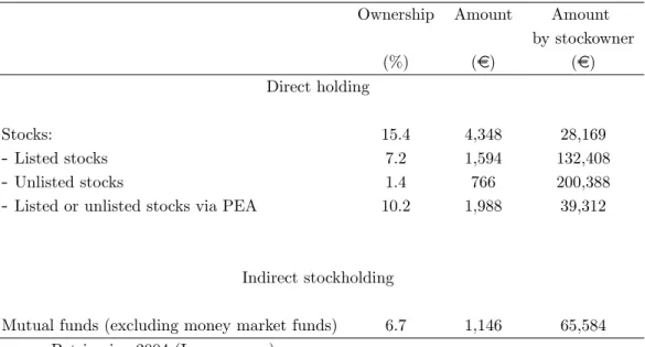
Table 1 below reports households’stockholding in France. The fraction of households with direct stockholding is about 15.4 percent. Around 7 percent of households have listed shares, 1.4 percent hold non-listed shares and 10.2 percent own shares via a PEA (Stocks’ saving account). The proportion of households with indirect stockholding -mainly through mutual funds- is around 6.7 percent. It follows that
16Heaton and Lucas (2000) argue that such a positive correlation re‡ect an indirect …nancing of
stockholding through leverage.
the upper bound of (direct or indirect) stockownership in France is estimated to be around 20 percent of the population. The average amount invested in (direct) stocks is about 4,350 euros (28,000 euros among direct stockholders) and households invest on average 1,146 euros in mutual funds (65,600 euros among owners).
Compared to the U.S., stock market participation remains limited in France. For the same surveyed year (2004), using the Survey of Consumer Finances, Bucks et al. (2009) report that the fraction of households holding directly or indirectly publicly traded stocks is about 50% in the U.S. This lower participation in stock markets is more generally observed in Europe, except in Sweden and in the U.K. (See Guiso et al., 2003).
Table 1. Stockholding in France
Ownership Amount Amount
by stockowner (%) (e) (e) Direct holding Stocks: 15.4 4,348 28,169 - Listed stocks 7.2 1,594 132,408 - Unlisted stocks 1.4 766 200,388
- Listed or unlisted stocks via PEA 10.2 1,988 39,312
Indirect stockholding
Mutual funds (excluding money market funds) 6.7 1,146 65,584
Source: Patrimoine 2004 (Insee survey)
The proportion of owner-occupiers of their main residence is about 55% (see graph 1). This rate varies a lot according to household’s age: very few young households own their main residence (about 20% of the 25-29 years old), then this rate increases until 70 years old. Our cross-section dataset does not allow us to disentangle between the life-cycle e¤ects and the generation e¤ects behind this pattern. The age e¤ect can be due to heterogeneity in the access to credit market, down-payment constraints more pregnant for young households or to the size of family (and children’age), etc, while at the same time, each generation of households encounters speci…c economic conditions especially as regards employment, growth, credit conditions and housing policies for a given age.
Graph 1. Percentage of homeowners and stockholders by age 0% 10% 20% 30% 40% 50% 60% 70% less than 25 25-29 30-34 35-39 40-44 45-49 50-54 55-59 60-64 65-69 70-74 older than 75 % of homeowners
% of stockholders (direct or indirect) % of stockholders (direct only)
Source: Patrimoine 2004 (Insee survey)
3.2
The sample
In addition to the composition of households’wealth, a part of the questionnaire give us a general idea of individuals’degree of exposure and aversion to risk, as subjec-tively perceived and assessed by respondents. It consists of a recto-verso questionnaire which was distributed to the interviewees at the end of the …rst interview. This page submitted to the whole sample must be …lled in individually by the interviewee and his/her spouse (if applicable) and returned by post to Insee. Only 4,262 individuals answered to this questionnaire (corresponding to 3,872 households).17 The content
is slightly di¤erent for employed persons than for unemployed or non working per-sons. More speci…cally, it asks the former to assess their short and long-term risks of unemployment, as well as the likely change in their future income over the next 5 years. In addition, a simple two-stage lottery game enables us to divide the individ-uals into four groups according to their degree of relative risk aversion following the methodology of Barsky et al. (1997).
17Arrondel (2009) shows that respondents are more educated, more often white-collar workers and
have less children. Although these relatively small di¤erences explain why the selected sample owns more often risky assets, the average share of …nancial wealth invested in risky assets is similar in both samples.
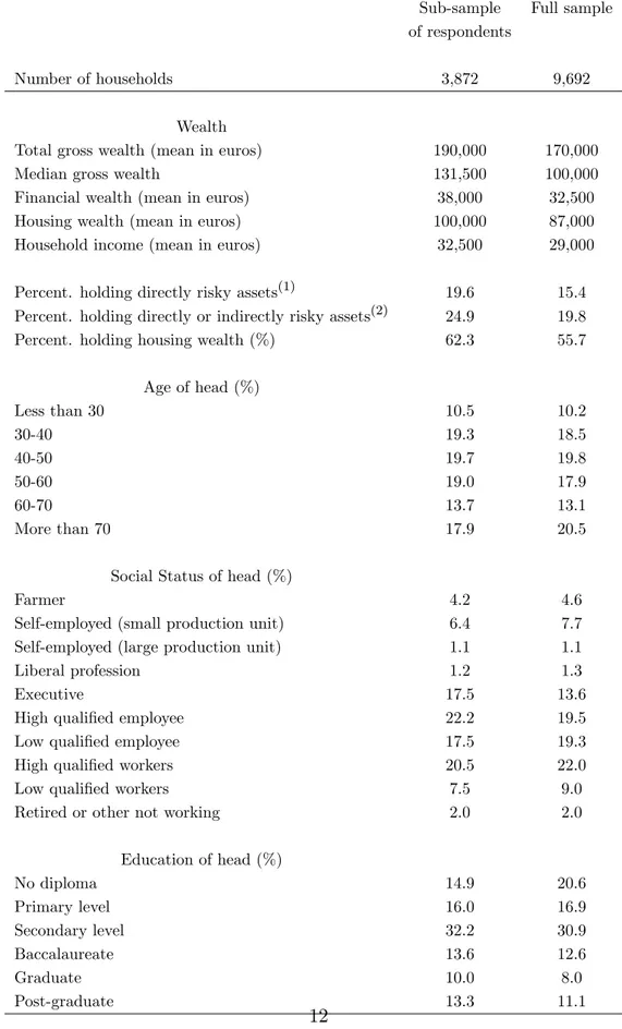
3.2.1 Comparison full sample versus econometric sample
In the Table 2, we report descriptive statistics for the whole sample of 9,692 house-holds which is representative of French househouse-holds and for our sub-sample of 3,872 respondents to the additional questions about risk attitude. There are some dif-ferences between the two samples: the sub-sample of respondents to the additional questionnaire seem to be more educated; they are more often white-collar workers and less often single and have more children. These di¤erences explain why the respon-dents are more wealthy (+ 12 percent for gross wealth, +17% for …nancial wealth) and earn more money at work (+ 12 percent).
These di¤erences in socioeconomic characteristics explain also why the sample of respondents own more often risky assets and are more frequently homeowner. The probability of owning risky assets is higher among the respondents than in the total sample (+4.2 percentage points for direct stockholding and +5.1 percentage points for direct or indirect stockholding). Concerning main residence, the percentage of homeowner is 6.6% higher for respondent and, consequently, housing wealth is 15% more important for this population.
As we are interested in studying the link between stockholding and real estate exposure to risk, the sub-sample of respondents is restricted to homeowners for the econometric analysis18.
18After some necessary cleaning our econometric sample include 1855 households. In addition,
robustness cheks are done on the full sample of respondents to the additionnal questionnaire (2248 households, renters and owners).
Table 2. Samples characteristics
Sub-sample Full sample of respondents
Number of households 3,872 9,692
Wealth
Total gross wealth (mean in euros) 190,000 170,000
Median gross wealth 131,500 100,000
Financial wealth (mean in euros) 38,000 32,500
Housing wealth (mean in euros) 100,000 87,000
Household income (mean in euros) 32,500 29,000
Percent. holding directly risky assets(1) 19.6 15.4
Percent. holding directly or indirectly risky assets(2) 24.9 19.8
Percent. holding housing wealth (%) 62.3 55.7
Age of head (%) Less than 30 10.5 10.2 30-40 19.3 18.5 40-50 19.7 19.8 50-60 19.0 17.9 60-70 13.7 13.1 More than 70 17.9 20.5
Social Status of head (%)
Farmer 4.2 4.6
Self-employed (small production unit) 6.4 7.7
Self-employed (large production unit) 1.1 1.1
Liberal profession 1.2 1.3
Executive 17.5 13.6
High quali…ed employee 22.2 19.5
Low quali…ed employee 17.5 19.3
High quali…ed workers 20.5 22.0
Low quali…ed workers 7.5 9.0
Retired or other not working 2.0 2.0
Education of head (%) No diploma 14.9 20.6 Primary level 16.0 16.9 Secondary level 32.2 30.9 Baccalaureate 13.6 12.6 Graduate 10.0 8.0 Post-graduate 13.3 11.1 12
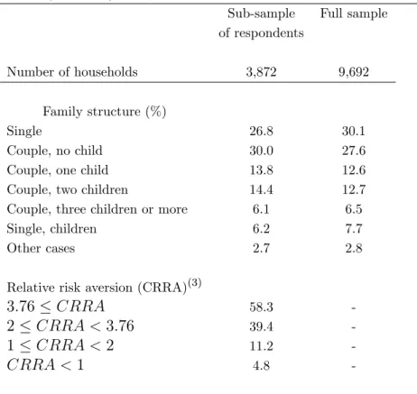
Table 2 (continued). Samples characteristics
Sub-sample Full sample of respondents
Number of households 3,872 9,692
Family structure (%)
Single 26.8 30.1
Couple, no child 30.0 27.6
Couple, one child 13.8 12.6
Couple, two children 14.4 12.7
Couple, three children or more 6.1 6.5
Single, children 6.2 7.7
Other cases 2.7 2.8
Relative risk aversion (CRRA)(3)
3:76 CRRA 58.3
-2 CRRA < 3:76 39.4
-1 CRRA < 2 11.2
-CRRA < 1 4.8
-Source: Patrimoine 2004 (Insee survey)
(1) Direct stockholding: households hold equities directly
(2) Direct or indirect stockholding: households hold equities directly or through mutual funds (3) The measure of risk aversion is described below.
3.2.2 Background risks
As previously stated, the Insee wealth survey allows us to take into account vari-ous background risks faced by the hvari-ousehold: income, unemployment, real estate, business.
Measure of income risk
We construct a proxy for the subjective variance of household income by following Guiso et al. (1996), i.e. each income recipient was asked to attribute probability weights (100 points) to given intervals of real income increases 5 years ahead of the interview (Arrondel, 2009). The sample average of expected income growth (around 1.1%) is roughly consistent with French time series evidence for the preceding period (around 1.8% for 1990-96). The mean of the standard error of anticipated income shocks19 (around 4.3% of current earnings) is closed to the estimates reported by
19Assuming that …ve years ahead expected real income is y
t+5= yt(1 + g), the formula of the
Guiso et al. (1996), but surprisingly low when compared to panel data estimates.20 Unreported Tobit regressions (Arrondel, 2009) show that households with higher uncertainty have had health problems and/or su¤ered unemployment in the past, are younger, less risk averse and more often self-employed (excluding farmers).
Measure of unemployment risk ( )
Each respondent has to evaluate the chances to lose his/her job in the …ve next years. The question is as follows: "How do you imagine your future employment within the next 5 years:
1) There is little or no risk that you will lose your job;
2) There is a possibility that you may lose your job (small risk); 3) It is probable that you will lose your job (considerably high risk); 4) It is certain, or almost certain, that you will lose your job".
By making simple assumptions, this information can be used to derive a measure of income variance: with an unemployment insurance replacement rate equal to zero, and assuming no changes in earnings if the respondent does not lose his/her job, it is easy to show that the variance of earnings is equal to p(1 p)Y2 where p is the subjective probability of losing the job and Y is income. If the replacement rate is equal to , the variance of income becomes p(1 p)(1 2)Y2. So we introduce this
subjective measure of unemployment risk in our risky asset demand equation.
Measure of exposure to real estate risk
Following Yamashita (2003), Cocco (2004) and Yao and Zhang (2005) we take into account the homeowners’exposure to real estate risk by introducing the ratio of housing wealth to net worth, the ratio of housing debt to net wealth and the ratio of mortgage payments to income (h variables).
As housing wealth measure, we use the value of the main residence, the net worth is total wealth less total debt (mortgages for main residence and other properties, consumption loans, professional loans).
The theoretical literature emphasize the two opposite e¤ects that housing wealth may have on stockholding. On the one hand, when reimbursing their loans contracted to buy their main residence, households increase their net wealth and reduce their global exposure to risk, thus they are more prone to rebalance their portfolio to invest in risky …nancial assets. On the other hand, owning real estate has a diversi…cation e¤ect on the household’s portfolio and thus may encourage stockholding. The graph g is the expected growth rate of real income and g2its variance. The frequency distribution for the
normalized standard deviation y=ytshows that 45.8% of the households hold point expectations.
Only 10% display a ratio above 12.5% of current earnings.
20The gap between both is commonly explained by overestimation of true ‘uncertainty’in
econo-metric regressions, neglected within interval variation, underreporting of the probability of very low income events and/or measurement error in survey responses. See Guiso et al. (1996, 2001) or Lusardi (1997) for details, and more recently Dominitz (2001) or Manski (2004) for a reassessment.
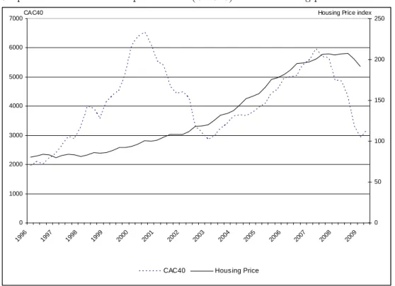
2 below draws the evolution of stock and housing prices in France since 1996. They exhibit a signi…cant positive correlation (equal to 0.3) that is not in favour of the diversi…cation e¤ect
Graph 2. Evolution of stock prices index (CAC40) and the housing price index in France
0 1000 2000 3000 4000 5000 6000 7000 1996 1997 1998 1999 2000 2001 2002 2003 2004 2005 2006 2007 2008 2009 CAC40 Housing Price index
0 50 100 150 200 250
CAC40 Housing Price
Concerning the housing debt variables, we expect a positive e¤ects as found in previous studies. This positive link re‡ect a"permanent income e¤ect": household with high human income are both prone to get loans to acquire housing assets and to invest in stocks.
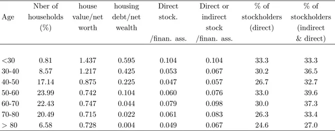
Table 3 reports some sample statistics calculated by age group computed from insee survey. As expected, we observe a decrease in both the ratios of house value and housing debt to net wealth with age. Before 40 years old, the ratio of housing to net worth is greater than one re‡ecting the households’leverage position (housing debt represents about 42% of households net wealth). Then, the housing debt becomes to be reimbursed and the real estate risk exposure decreases. At the end of life, the housing debt is fully reimbursed while house value represents more than 70% of net wealth for homeowners. The other columns reports the importance of stockholding across ages. It is di¢ cult to draw a simple relation between the exposure to housing risk and stockholding (ownership and amount) with these simple statistics.
Table 3. Wealth and portfolio composition by age groups (econometric sample: homeowners)
Nber of house housing Direct Direct or % of % of
Age households value/net debt/net stock. indirect stockholders stockholders
(%) worth wealth stock (direct) (indirect
/…nan. ass. /…nan. ass. & direct)
<30 0.81 1.437 0.595 0.104 0.104 33.3 33.3 30-40 8.57 1.217 0.425 0.053 0.067 30.2 36.5 40-50 17.14 0.875 0.225 0.047 0.057 26.7 32.7 50-60 23.99 0.742 0.104 0.060 0.076 33.0 39.6 60-70 22.43 0.747 0.044 0.079 0.098 30.0 37.3 70-80 20.49 0.715 0.022 0.061 0.083 26.3 33.4 > 80 6.58 0.728 0.004 0.049 0.067 24.6 27.0
Source: Patrimoine 2004 (Insee survey)
Finally, we take into account a possible impact of business risk on households …nancial investments with a dummy identifying self-employed heads of households and the ratio of business wealth to net wealth. For people owning a business, the business wealth represents about 31% of their net wealth. As for housing wealth, there is a trade-o¤ between the diversi…cation bene…t of owning a business and the bene…t of holding liquid …nancial assets. The diversi…cation bene…t encourages to hold business wealth and to invest in …nancial stock markets while owning such an illiquid and risky asset may discourage to invest in stocks.
3.2.3 Measure of risk aversion ( )
As in Barsky et al. (1997), a measure of risk aversion is obtained by asking respon-dents about their willingness to gamble on lifetime income, say R. The subject is o¤ered various job contracts in the form of a lottery, with one chance out of two to
earn twice more and one chance out of two to earn only R (with a parameter
inferior to one). In the standard framework assuming expected utility, the subject with indirect utility V will prefer the contract to the sure gain R only and only if :
1
2V (2R) + 1
2V ( R) V (R) (1)
with V assumed to be isoelastic of parameter . A range of variation for relative risk aversion can be determined by varying the value of : for instance, if the subject refuse the job contract for = 2=3, but accepts it for = 4=5, the value of its parameter is in the interval [2; 3:76[.
The outcome is a range measure (in four brackets) for the relative risk aversion coe¢ cient ( ) under the assumption that preferences are strictly risk averse and of the CRRA type. Out of the 3,488 respondents, 58.3% are very risk averse ( 3:76)
and 26.6% are highly so (2 3:76). 10.2% display moderate aversion (1 2)
while only 4.8% quali…ed as low risk averse ( < 1). Controlling for demographic and economic factors, unreported evidence (Arrondel, 2009) shows that those who are more risk tolerant are also more willing to take risk in …nancial decisions and more likely to become self-employed (excluding farmers).
4
Econometric speci…cation
We consider the following relation for the share of risky assets in …nancial wealth: Ai
Fi
= g ( i; i; hi; Xi) + "i (2)
where Ai( 0) is the demand for risky assets and Fi is total …nancial wealth of
the household i, 2 is the subjective earnings variance,
i is the coe¢ cient of relative
risk aversion, h represents the housing variables and Xi is a vector of other variables
which in‡uence the demand for risky investments. "i is an error term. Here, income
risk is assumed to be exogenous as in recent models of portfolio choice.
Our dependent variable is the value of stocks directly held to …nancial assets.21 The set of explanatory variables X is determined by the classical portfolio choice model as well as its extensions. In portfolio choice models where capital markets are imperfect (transaction costs, holding costs, imperfect information) portfolios are incomplete (King and Leape, 1998). So portfolio choice depends on household’s income and wealth (to …nance transaction and information costs) and on the stock of …nancial information (proxied by age, education, parents’wealth composition).
We also introduce the measure of risk aversion described above as well as an indi-cator of time preference. It is obtained by asking households to give their subjective position on a scale of time preference. More precisely we ask: "On a scale of zero to ten, where would you place yourself between the following two "extreme" descriptions ?:
0 : persons who live day by day and take life as it comes, who don’t think too much about tomorrow nor worry about the future;
10: persons who are preoccupied by their future (even their distant future) and whose mind is well set on what they want to be or do later in on life."
As presented before, we also introduce the following variables to account for the impact of housing on stockholding: the ratio of housing value to net wealth, the ratio of housing debt to net wealth and the ratio of mortgage annuities on income.
We also take into account other sources of future exogenous risk, especially on family (we control by marital status and number of children at home or away from home). Finally, we introduce the nature of (present or past) professional activity (employee vs. self-employed as well as the ratio of business wealth to net wealth).
The e¤ect of age included in X is polysemous (Arrondel and Masson, 1996). Bodie et al. (1992) show that the young enjoy greater labor ‡exibility than the old and may therefore be more likely to hold risky assets; Gollier and Zeckhauser (1997) show that young households take on relatively more portfolio risk than older households if (and only if) absolute risk tolerance is convex; King and Leape (1987) stress that …nancial information is acquired slowly along individual’s life, a fact that can explain why the young hold a less diversi…ed portfolio than the old: the young are more likely to be liquidity constrained and so less willing to take risk when choosing their portfolio.
A simple OLS regression leads to inconsistent estimates due to the fact that a signi…cant proportion of households does not own risky assets. In the same way, OLS regressions on the restricted sample of investors who hold risky assets is subject to selection bias (Heckman, 1976). We handle the selection bias by estimating a Tobit model on the share of risky assets where the lower limit is zero22.
4.1
Main results
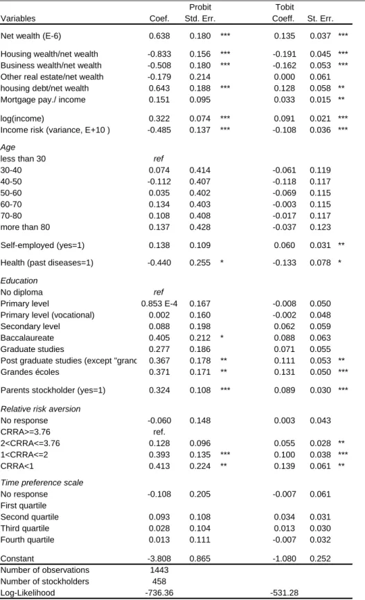
Table 4 reports probit and tobit estimates.
The positive e¤ect of total net wealth in the probit model is consistent with the presence of …xed transaction costs when homeowners decide to own stocks or not. An increase in the amount of their total net wealth from the 10th percentile (around 72,000 euros) to the 90th percentile (around 615,600 euros) increases the probability of being a stockholder by 7.4 percentage points, when holding the other variables in the regression constant at their means. At the same time, the ratio of stocks to …nancial assets increases from 4.5% to 6.5%. This positive e¤ect of net wealth on the ratio of stocks to net wealth re‡ects that these risky …nancial assets can be viewed as a luxury good:
The stock of information inherited from parents proxied by the ownership of the same assets in parents’ wealth increases also the probability of risky assets owner-ship. Households whose parents owned stocks are about 9.6 percentage points more likely to hold stocks directly, again keeping the other regression variables constant at their means. Moreover, education has a strong positive e¤ect on stockholding: with graduate households stockownership increases by 13.7% compared to those without diploma and the share of …nancial wealth invested in stocks is twice (4.1 versus 6.9). Concerning human resources, we …rst note a positive mean-e¤ect of non …nancial income on the probability of stock market participation. Moving a household from the 10th to the 90th percentile of the labor income distribution increases the probability of being a stockholder by 14.6 percentage points. We do not …nd any signi…cant e¤ect of age nor of the indicator of time preference in both the probit and tobit equations.
22However, Tobit estimation constrains the determinants of whether to hold risky assets or not
and if so how much to depend on the same set of variables,
Table 4. Estimates of direct stockholding (discrete and continuous choice)
Probit Tobit
Variables Coef. Std. Err. Coeff. St. Err. Net wealth (E-6) 0.638 0.180 *** 0.135 0.037 *** Housing wealth/net wealth -0.833 0.156 *** -0.191 0.045 *** Business wealth/net wealth -0.508 0.180 *** -0.162 0.053 *** Other real estate/net wealth -0.179 0.214 0.000 0.061 housing debt/net wealth 0.643 0.188 *** 0.128 0.058 ** Mortgage pay./ income 0.151 0.095 0.033 0.015 ** log(income) 0.322 0.074 *** 0.091 0.021 *** Income risk (variance, E+10 ) -0.485 0.137 *** -0.108 0.036 ***
Age
less than 30 ref
30-40 0.074 0.414 -0.061 0.119 40-50 -0.112 0.407 -0.118 0.117 50-60 0.035 0.402 -0.069 0.115 60-70 0.134 0.403 -0.003 0.115 70-80 0.108 0.408 -0.017 0.117 more than 80 0.137 0.428 -0.037 0.123 Self-employed (yes=1) 0.138 0.109 0.060 0.031 ** Health (past diseases=1) -0.440 0.255 * -0.133 0.078 *
Education
No diploma ref
Primary level 0.853 E-4 0.167 -0.008 0.050 Primary level (vocational) 0.002 0.160 -0.002 0.048 Secondary level 0.088 0.198 0.062 0.059 Baccalaureate 0.405 0.212 * 0.088 0.063 Graduate studies 0.277 0.186 0.071 0.055 Post graduate studies (except "grandes écoles"0.367 0.178 ** 0.111 0.053 ** Grandes écoles 0.371 0.171 ** 0.131 0.050 *** Parents stockholder (yes=1) 0.324 0.108 *** 0.089 0.030 ***
Relative risk aversion
No response -0.060 0.148 0.003 0.043 CRRA>=3.76 ref.
2<CRRA<=3.76 0.128 0.096 0.055 0.028 ** 1<CRRA<=2 0.393 0.135 *** 0.100 0.038 *** CRRA<1 0.413 0.224 ** 0.139 0.061 **
Time preference scale
No response -0.108 0.205 -0.007 0.061 First quartile Second quartile 0.093 0.108 0.034 0.031 Third quartile 0.028 0.104 0.013 0.030 Fourth quartile 0.013 0.111 -0.007 0.032 Constant -3.808 0.865 -1.080 0.252 Number of observations 1443 Number of stockholders 458 Log-Likelihood -736.36 -531.28
Source: Patrimoine 2004 (Insee survey)
The dependent variable in the probit model is a dichotomous variable equals to one if households hold directly stocks.
The e¤ect of individual measures of risk aversion has the expected sign: households who are classi…ed in the group of high risk averters were, ceteris paribus about 15.2 percentage points less likely to hold stocks directly (relatively to the group of low risk averters), and the share of …nancial wealth invested in stocks is twice (4.6% versus 9%).
The coe¢ cient of the expected variance of income is negative and signi…cantly di¤erent from zero: households whose future income is more risky are also those who invest less in risky assets. In other words, the exogenous income risk and the en-dogenous risk associated with households’decision to include stocks in their portfolio appear to be substitutes. However, the size of the e¤ect is limited (households who have no risk on their labor income were, ceteris paribus, about 0.6 percentage points less likely to hold stocks directly compared to households who are in the highest risky income decile). We note also a negative e¤ect of health past diseases on the probability of stock ownership.
Being self-employed or having a business wealth seem to be a risk that house-holds take into account when deciding to participate in stockmarket: househouse-holds with businesses moderate their total exposure to risk by reducing their equity invest-ment. Being self-employed decreases the probability to participate in stockmarkets by 6.3 percentage points. Moreover, business wealth crowds out the wealth invested in stocks: increasing the business from the …rst to the last decile decreases the likelihood to own stocks by 4.2 percentage points.
All housing-related variables have signi…cant e¤ects on homeowners stockmar-ket participation decisions and investment. Housing wealth has a crucial impact on stockholding. For a homeowner, moving from the …rst decile of the distribution of the housing wealth to the last one increases the probability to own stocks by 19.2 percentage point. Moreover, the home-value to net worth ratio a¤ects negatively the ratio of equity to net wealth re‡ecting a liquidity e¤ect: a higher home-value to net wealth ratio implies less liquid wealth is available for …nancial investments. For instance, households with a ratio of housing wealth to net wealth greater than 1.3 (ninth decile of the distribution) invest 3.1% of their …nancial wealth in stocks while households with an housing ratio smaller than 0.3 (…rst decile of the distribution) invest 8.3 of their …nancial wealth in risky assets.
As previously stated by other empirical studies, we obtain signi…cant positive e¤ects for the housing debt to net wealth ratio and the annual mortgage payment to income ratio. An increase in the housing debt ratio from the …rst to the ninth decile increases the probability to own stocks by 4.9 percent point. This can be interpreted as a permanent income e¤ect: for a given housing wealth, more educated household that enjoy also higher future expected labor income are able to borrow more (for home acquisition), and are also more prone to invest more in stockmarkets. Moreover, a higher "human wealth" can be considered as a less risky and more liquid asset than stocks and thus leads to invest in more risky …nancial assets like equities.
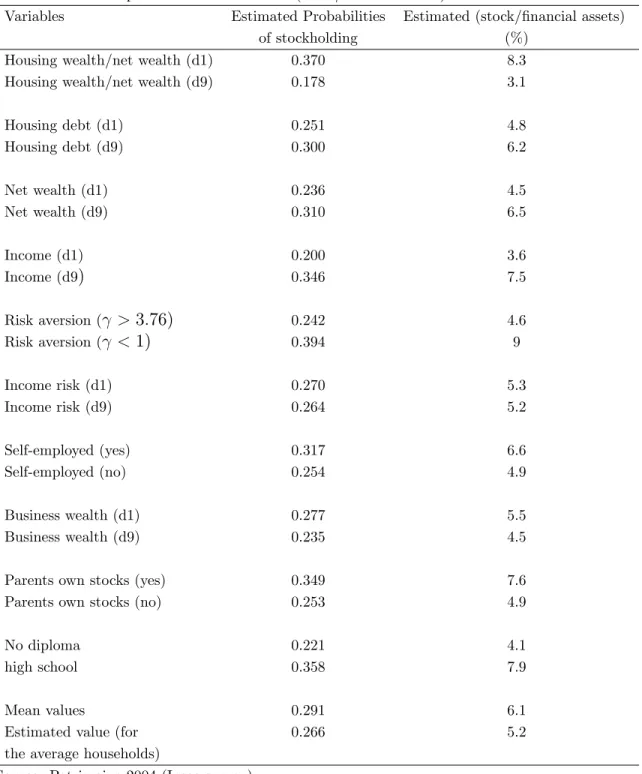
Table 5. Estimated probabilities and amount (stock/…nancial assets) of stock demand
Variables Estimated Probabilities Estimated (stock/…nancial assets)
of stockholding (%)
Housing wealth/net wealth (d1) 0.370 8.3
Housing wealth/net wealth (d9) 0.178 3.1
Housing debt (d1) 0.251 4.8 Housing debt (d9) 0.300 6.2 Net wealth (d1) 0.236 4.5 Net wealth (d9) 0.310 6.5 Income (d1) 0.200 3.6 Income (d9) 0.346 7.5 Risk aversion ( > 3:76) 0.242 4.6 Risk aversion ( < 1) 0.394 9 Income risk (d1) 0.270 5.3 Income risk (d9) 0.264 5.2 Self-employed (yes) 0.317 6.6 Self-employed (no) 0.254 4.9 Business wealth (d1) 0.277 5.5 Business wealth (d9) 0.235 4.5
Parents own stocks (yes) 0.349 7.6
Parents own stocks (no) 0.253 4.9
No diploma 0.221 4.1
high school 0.358 7.9
Mean values 0.291 6.1
Estimated value (for 0.266 5.2
the average households)
Source: Patrimoine 2004 (Insee survey)
Note: This table is computed using the tobit estimates presented in table 4. (d1) : indicates the value computed for the …rst decile of the variable (d9) : indicates the value computed for the last decile of the variable
4.2
Robustness checks
We conduct various other regressions to test the robustness of our results.
First, we try to assess whether the insigni…cant coe¢ cients for age can be due to a colinearity problem with housing variables (as homeownership and age are correlated). However, when excluding housing variables, the age variable remains insigni…cant.
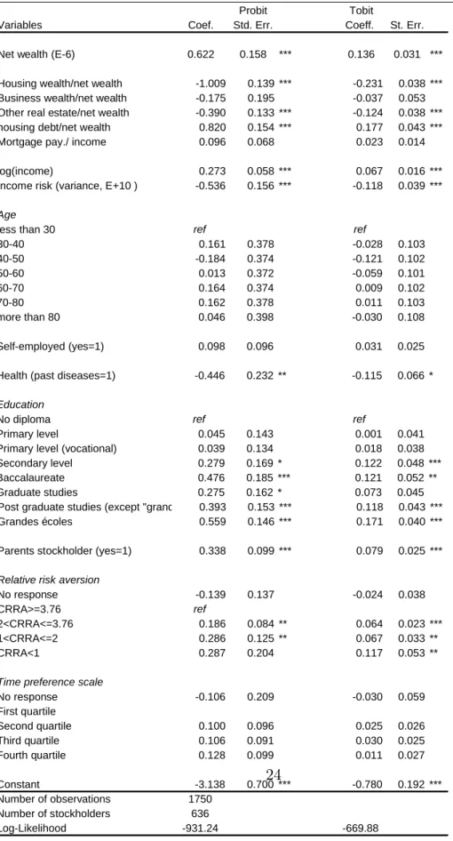
Second, we run the regression by considering both direct and indirect stockholding (instead of only direct stockholding) as the dependent variable (see table A1). We obtain similar e¤ects.
Third, as we are interested in the impact of housing wealth on stockholding, the sample is restricted to homeowners (as done by Cocco (2004) for instance). However, one may be interested in the determinants of stockholding for the full population (not only homeowners). So we run a similar regression on the full subsample of respondents (i.e. owners and renters) and we add a dummy variable to account for the households tenure status. As one may wonder about the endogeneity of the households tenure status, we estimate simultaneously the demand for stocks and a probit equation describing the likelihood to be homeowner. The probability of being homeowner is explained by housing consumption need (size of family), whether the households bene…ts from past inheritance and heterogenity in local housing prices (taken into account through the urbain or rural environment and the urban size).
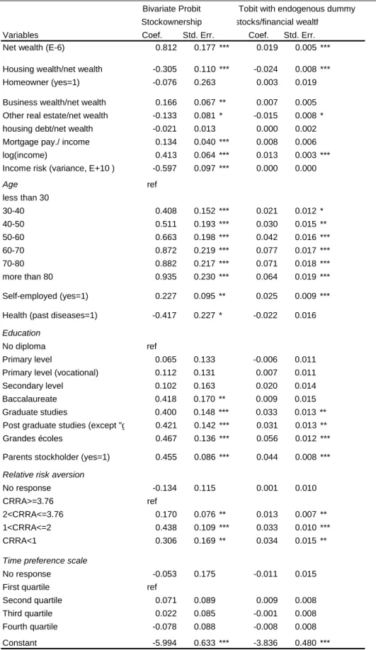
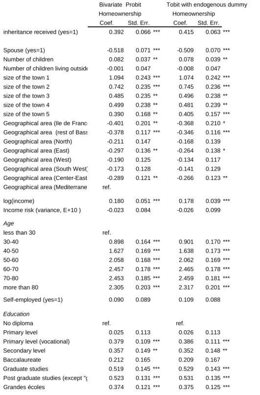
The results are presented in table A2: the …rst column reports the bivariate probit estimates of the likelihood to be respectively stockholders and homeowners, the second column reports the tobit estimates of the stockholding to …nancial assets ratio with the endogenous tenure status dummy. The results con…rm the previous results about the impact of real estate exposure to stockholding. In particular, the ratio of housing on net wealth remains signi…cantly negative. The main di¤erence with the estimates on the sub-sample of homeowners lies in the age e¤ect. Now we obtain an increasing stockholding along the life-cycle.
5
Conclusion
One of the main puzzle faced by the empirical literature on wealth portfolio deals with the so-call "equity premium puzzle". How to explain the low participation of households to the stockmarkets, and when they do participate, why do they under-invest compared to the main results of the theoretical models? Indeed, the standard portfolio theory predicts that households’ portfolio are fully diversi…ed and so in-vest in stocks. Various explanations of this puzzle are inin-vestigated in the literature: transactions costs, unavoidable risks on the job market, liquidity constraints, labour ‡exibility. In this paper, we focused on a more recent approach that links housing investment and stockmarkets participation. Housing represents the main assets in the households’wealth and is associated with various constraints and risks (housing price evolution, illiquidity, indebtedness over a long period). These characteristics may lead
households to limit their investment in risky …nancial assets by temperance.
We use the French wealth survey (Enquête Patrimoine2004, Insee) that give us de-tailed information on households portfolio composition (housing and …nancial wealth, mortgages), socio-demographic variables, and several measures of attitudes (risk aver-sion, scales on time preference) and exposition to various risks (income, unemploy-ment, health, business).
We obtain a strong impact of real estate exposure to risk on stockholding. First, housing wealth crowds out stock market participation re‡ecting a liquidity e¤ect: a higher home-value to net wealth ratio implies less liquid wealth is available for …nancial investments. This impact is very strong: for example, a homeowner who moves from the …rst decile of the distribution of the housing wealth to the last one increases his probability to own stocks from 0.18 to 0.37.
Among the other signi…cant determinants of the equity premium puzzle, we em-phasize the role of transaction and information costs, the attitude toward risk and the exposition to various risks (we …nd signi…cant e¤ect of income, unemployment and business risks) in limiting investments in stocks.
Finally, this paper may help to evaluate the impact of the current economic crisis that reinforces households exposure to risks and which associated with uncertainty about housing market evolution on households wealth allocation.
6
Appendix
Table A1. Estimates of direct and indirect stockholding (discrete and continuous choice)
Probit Tobit
Variables Coef. Std. Err. Coeff. St. Err. Net wealth (E-6) 0.622 0.158 *** 0.136 0.031 *** Housing wealth/net wealth -1.009 0.139 *** -0.231 0.038 *** Business wealth/net wealth -0.175 0.195 -0.037 0.053 Other real estate/net wealth -0.390 0.133 *** -0.124 0.038 *** housing debt/net wealth 0.820 0.154 *** 0.177 0.043 *** Mortgage pay./ income 0.096 0.068 0.023 0.014 log(income) 0.273 0.058 *** 0.067 0.016 *** Income risk (variance, E+10 ) -0.536 0.156 *** -0.118 0.039 ***
Age
less than 30 ref ref
30-40 0.161 0.378 -0.028 0.103 40-50 -0.184 0.374 -0.121 0.102 50-60 0.013 0.372 -0.059 0.101 60-70 0.164 0.374 0.009 0.102 70-80 0.162 0.378 0.011 0.103 more than 80 0.046 0.398 -0.030 0.108 Self-employed (yes=1) 0.098 0.096 0.031 0.025 Health (past diseases=1) -0.446 0.232 ** -0.115 0.066 *
Education
No diploma ref ref
Primary level 0.045 0.143 0.001 0.041 Primary level (vocational) 0.039 0.134 0.018 0.038 Secondary level 0.279 0.169 * 0.122 0.048 *** Baccalaureate 0.476 0.185 *** 0.121 0.052 ** Graduate studies 0.275 0.162 * 0.073 0.045 Post graduate studies (except "grandes écoles"0.393 0.153 *** 0.118 0.043 *** Grandes écoles 0.559 0.146 *** 0.171 0.040 *** Parents stockholder (yes=1) 0.338 0.099 *** 0.079 0.025 ***
Relative risk aversion
No response -0.139 0.137 -0.024 0.038 CRRA>=3.76 ref
2<CRRA<=3.76 0.186 0.084 ** 0.064 0.023 *** 1<CRRA<=2 0.286 0.125 ** 0.067 0.033 ** CRRA<1 0.287 0.204 0.117 0.053 **
Time preference scale
No response -0.106 0.209 -0.030 0.059 First quartile Second quartile 0.100 0.096 0.025 0.026 Third quartile 0.106 0.091 0.030 0.025 Fourth quartile 0.128 0.099 0.011 0.027 Constant -3.138 0.700 *** -0.780 0.192 *** Number of observations 1750 Number of stockholders 636 Log-Likelihood -931.24 -669.88
Source: Patrimoine 2004 (Insee survey) Notes:
The dependent variable in the probit model is a dichotomous variable equals to one if housholds hold directly or indirectly stocks.
The dependent variables in the tobit model is the ratio of direct and indirect stockholding on …nancial assets. */**/*** indicates the level the variable is statistically signi…cant at respectively 10/5/1 percent.
Table A2. Simultaneous estimates of stockholding and tenure choice
Tobit with endogenous dummy Variables Coef. Std. Err. Coef. Std. Err.
Net wealth (E-6) 0.812 0.177 *** 0.019 0.005 *** Housing wealth/net wealth -0.305 0.110 *** -0.024 0.008 *** Homeowner (yes=1) -0.076 0.263 0.003 0.019 Business wealth/net wealth 0.166 0.067 ** 0.007 0.005 Other real estate/net wealth -0.133 0.081 * -0.015 0.008 * housing debt/net wealth -0.021 0.013 0.000 0.002 Mortgage pay./ income 0.134 0.040 *** 0.008 0.006 log(income) 0.413 0.064 *** 0.013 0.003 *** Income risk (variance, E+10 ) -0.597 0.097 *** 0.000 0.000
Age ref less than 30 30-40 0.408 0.152 *** 0.021 0.012 * 40-50 0.511 0.193 *** 0.030 0.015 ** 50-60 0.663 0.198 *** 0.042 0.016 *** 60-70 0.872 0.219 *** 0.077 0.017 *** 70-80 0.882 0.217 *** 0.071 0.018 *** more than 80 0.935 0.230 *** 0.064 0.019 *** Self-employed (yes=1) 0.227 0.095 ** 0.025 0.009 *** Health (past diseases=1) -0.417 0.227 * -0.022 0.016
Education
No diploma ref
Primary level 0.065 0.133 -0.006 0.011 Primary level (vocational) 0.112 0.131 0.007 0.011 Secondary level 0.102 0.163 0.020 0.014 Baccalaureate 0.418 0.170 ** 0.009 0.015 Graduate studies 0.400 0.148 *** 0.033 0.013 ** Post graduate studies (except "grandes écoles"0.421 0.142 *** 0.031 0.013 ** Grandes écoles 0.467 0.136 *** 0.056 0.012 *** Parents stockholder (yes=1) 0.455 0.086 *** 0.044 0.008 ***
Relative risk aversion
No response -0.134 0.115 0.001 0.010 CRRA>=3.76 ref
2<CRRA<=3.76 0.170 0.076 ** 0.013 0.007 ** 1<CRRA<=2 0.438 0.109 *** 0.033 0.010 *** CRRA<1 0.306 0.169 ** 0.034 0.015 **
Time preference scale
No response -0.053 0.175 -0.011 0.015 First quartile ref
Second quartile 0.071 0.089 0.009 0.008 Third quartile 0.022 0.085 -0.001 0.008 Fourth quartile -0.078 0.088 -0.008 0.008 Constant -5.994 0.633 *** -3.836 0.480 ***
Bivariate Probit
Table A2 (continued). Simultaneous estimates of stockholding and tenure choice
Tobit with endogenous dummy Coef. Std. Err. Coef. Std. Err.
inheritance received (yes=1) 0.392 0.066 *** 0.415 0.063 *** Spouse (yes=1) -0.518 0.071 *** -0.509 0.070 *** Number of children 0.082 0.037 ** 0.078 0.039 ** Number of children living outside -0.001 0.047 -0.008 0.047 size of the town 1 1.094 0.243 *** 1.074 0.242 *** size of the town 2 0.742 0.235 *** 0.745 0.236 *** size of the town 3 0.485 0.235 ** 0.496 0.238 ** size of the town 4 0.499 0.238 ** 0.481 0.239 ** size of the town 5 0.390 0.168 ** 0.405 0.157 *** Geographical area (Ile de France) -0.401 0.201 ** -0.368 0.210 * Geographical area (rest of Bassin parisien)-0.378 0.117 *** -0.346 0.116 *** Geographical area (North) -0.211 0.147 -0.168 0.139 Geographical area (East) -0.297 0.136 ** -0.264 0.138 * Geographical area (West) -0.190 0.125 -0.134 0.117 Geographical area (South West) -0.173 0.128 -0.141 0.129 Geographical area (Center-East) -0.289 0.121 ** -0.266 0.123 ** Geographical area (Mediterranean cost)ref.
log(income) 0.180 0.051 *** 0.178 0.039 *** Income risk (variance, E+10 ) -0.023 0.084 -0.026 0.099
Age
less than 30 ref.
30-40 0.898 0.164 *** 0.901 0.170 *** 40-50 1.627 0.169 *** 1.638 0.173 *** 50-60 2.058 0.168 *** 2.062 0.169 *** 60-70 2.457 0.178 *** 2.465 0.178 *** 70-80 2.453 0.185 *** 2.459 0.181 *** more than 80 2.305 0.203 *** 2.317 0.201 *** Self-employed (yes=1) 0.090 0.089 0.109 0.088 Education
No diploma ref. ref.
Primary level 0.025 0.113 0.026 0.113 Primary level (vocational) 0.379 0.109 *** 0.386 0.111 *** Secondary level 0.357 0.149 ** 0.352 0.148 ** Baccalaureate 0.212 0.165 0.209 0.167 Graduate studies 0.519 0.145 *** 0.529 0.143 *** Post graduate studies (except "grandes écoles"0.523 0.131 *** 0.531 0.135 *** Grandes écoles 0.374 0.121 *** 0.375 0.125 ***
Homeownership Homeownership Bivariate Probit
Relative risk aversion
No response -0.257 0.107 ** -0.242 0.107 ** CRRA>=3.76 ref. ref.
2<CRRA<=3.76 -0.010 0.076 -0.006 0.079 1<CRRA<=2 -0.049 0.112 -0.044 0.109 CRRA<1 -0.267 0.154 * -0.266 0.162
Time preference scale
No response -0.086 0.158 -0.117 0.157 First quartile ref. ref.
Second quartile -0.056 0.088 -0.056 0.091 Third quartile -0.100 0.084 -0.110 0.085 Fourth quartile -0.225 0.083 *** -0.231 0.083 *** Rho 0.300 0.139 Rho*sigma 0.021 0.011 Log-likelihood -2254.290 Number of observations 2248.000
Source: Patrimoine 2004 (Insee survey)
*/**/*** indicates the level the variable is statistically signi…cant at respectively 10/5/1 percent.
References
[1] Alessie, R., Hochguertel, S. and van Soest, A. (2001). ”Household Portfolios in The Netherlands”, in Household Portfolios, Guiso L., Haliassos M. and T. Japelli eds, MIT Press.
[2] Arrondel, L. (2002). “Risk Management and Wealth Accumulation Behavior in France”, Economics Letters, vol. 74, 187-194.
[3] Arrondel, L. and Masson, A. (2003). ”Stockholding in France”, in Stocholding in Europe, Guiso L., Haliassos M. and T. Jappelli eds, Palgrave, Hampshire, pp. 75-109.
[4] Arrondel L., Lefebvre B. (2001). “Consumption and investment motives in hous-ing wealth accumulation : a French study”, Journal of Urban Economics, 50, p. 112-137.
[5] Arrondel, L. and Calvo-Pardo, H. (2009) “Les Français sont ils prudents?: pat-rimoine et risques sur le marché du travail”, Economie et Statistique, 417-417, p. 27-53.
[6] Arrow, K. J. (1965). Aspects of the Theory of Risk Bearing, Yrjo Jahnsson Lectures, The Academic Book Store, Helsinki.
[7] Barsky, R. B., Juster, T. F., Kimball, M. S. and Shapiro, M. D. (1997). “Prefer-ence Parameters and Behavioral Heterogeneity : an Experimental Approach in
the Health and Retirement Study”, Quarterly Journal of Economics, Vol. CXII, 537-580.
[8] Bodie, Z., Merton, R. et Samuelson, W.(1992). “Labor Supply Flexibility and Portfolio Choice in a Life Cycle Model”, Journal of Economic Dynamics and Control, 16, 427-449, 1992.
[9] Bucks, B. K, Kennickell, A. B, Mach, T. L., Moore K. B. (2009). “Changes in U.S. Family Finances from 2004 to 2007: Evidence from the Survey of Consumer Finances”, Federal Reserve Bulletin.
[10] Campbell, J.Y. and Viceira, L. M. (2002). Strategic Asset Allocation: Portfo-lio Choice for Long-Term Investors, Clarendon, Lectures in Economics, Oxford University Press.
[11] Cocco J. (2004) “Portfolio Choice in the presence of housing”, Review of Finan-cial Studies, 18-2, p. 535-566.
[12] Eeckhoudt, L., Gollier, C. (2001). “Are Independent Optimal Risks Substi-tutes?”, (mimeo) Toulouse.
[13] Eeckhoudt, L., Gollier, C. and Schlesinger, H. (1996). “Changes in Background Risk and Risk Taking Behavior”, Econometrica, vol. 64, pp. 683-689.
[14] Elmendorf, D. W. and Kimball, M. S. (2000). “Taxation of Labour Income and the Demand for Risky Assets”, International Economic Review, vol. 41, pp. 801-832.
[15] Flavin M., Yamashita T. (2002) “Owner-Occupied Housing and the Composition of the household portfolio”, American Economic Review, 92-1, p. 345-362. [16] Fratantoni, M. C. (2001) “Homeownership, commited expenditure risk, and the
stockholding puzzle”, Oxford Economic Papers, 53, 241-259. [17] Gollier Ch. (2001), The Economics of Risk and Time, MIT Press.
[18] Gollier, C. (2001). The Economics of Risk and Time, MIT Press, Cambridge. [19] Gollier, C. and Pratt, J. W. (1996). ”Weak Proper Risk Aversion and the
Tem-pering E¤ect of Background Risk”, Econometrica, vol. 64, pp. 1109-1123. [20] Gollier, C. and Zeckhauser R. (2002). ”Time Horizon and Portfolio Risk”,
Jour-nal of Risk and Uncertainty, 49(3), pp. 195-212.
[21] Guiso, L. and Paiella, M. (2000). ”Risk Aversion, Wealth and Financial Market”, mimeo.
[22] Guiso, L., Haliassos M. and Jappelli, T. (2001), Household Portfolios, MIT Press. [23] Guiso, L., Haliassos M. and Jappelli, T. (2003), Stocholding in Europe, Palgrave,
Hampshire.
[24] Guiso, L., Jappelli, T. and Terlizzese, D. (1992). ”Earnings Uncertainty and Precautionary Saving”, Journal of Monetary Economics, vol. 30, 307-338. [25] Guiso, L., Jappelli, T. and Terlizzese, D. (1996). ”Income Risk, Borrowing
Con-straints and Portfolio Choice”, American Economic Review, vol. 86, pp. 158-172. [26] Haliassos M., (2003), “Stockholding: Recent Lessons from Theory and Compu-tations”, in Stockholding in Europe, Edited by Luigi Guiso, Michael Haliassos and Tullio Jappelli, Palgrave Macmillan Publishers.
[27] Heaton J. and Lucas, D. (2000). ”Portfolio Choice in the Presence of Background Risk”, Economic Journal, vol. 110, 1-26.
[28] Heckman, J. J. (1976). ”The Common Structure of Statistical Models of Trunca-tion, Sample Selection and Limited Dependent Variables and a Simple Estimator for Such Models”, Annals of Economic and social Measurement, vol. 5, 475-492. [29] Kapteyn, A. and Teppa, F. (2002). ”Subjective Measures of Risk Aversion and
Portfolio Choice”, CENter Discussion paper n 2002-11, Tilburg.
[30] Saarimaa T. (2008) “Owner-occupied housing and demand for risky …nancial assets: some Finnish evidence”, Finnish Economic Papers, 21(1), 22-38.
[31] Kimball, Miles S, 1993. “Standard Risk Aversion”, Econometrica, vol. 61(3), pages 589-611.
[32] King, M. A et Leape, J. (1998), “Wealth and portfolio consumption: theory and evidence”, Journal of public economics, 69 (2). p 155-193.
[33] Kihlstrom, R.E., Romer, D. and Williams, S. (1981). ”Risk Aversion with Ran-dom Initial Wealth”, Econometrica, vol. 49, pp. 911-920.
[34] Kimball, M. S. (1990). ”Precautionary Saving in the Small and in the Large”, Econometrica, vol. 58, pp. 53-73.
[35] Kimball, M. S. (1993). ”Standard Risk Aversion”, Econometrica, vol. 61, pp. 589-611.
[36] King, M. A. and Leape, J. I. (1987) ”Asset Accumulation, Information, and the Life Cycle”, N.B.E.R. WP2392.
[37] King, M. A. and Leape, J. I. (1998). ”Wealth and Portfolio Composition: Theory and Evidence”, Journal of Public Economy, vol. 69, pp. 155-193.
[38] Koo, H.K. (1995). ”Consumption and Portfolio Selection with Labor Income: Evaluation of Human Capital”, mimeo, Olin School of Business, Washington University.
[39] Merton R. C. (1971), “Optimal Consumption and Portfolio Rules in a continuous-Time Model”, Journal of Economic Theory, vol. 3(4), p. 373-413. [40] Pratt, J. (1964). ”Risk aversion in the small and in the large”, Econometrica,
vol. 32, pp. 122-136.
[41] Pratt, J. and Zeckhauser R. (1987). ”Proper Risk Aversion”, Econometrica, vol. 55, pp. 143-154.
[42] Viceira, L. M. (2001). ”Optimal Portfolio Choice For Long-Horizon Investors With Nontradable Labor Income”, The Journal of Finance 56, pp. 433-470. [43] Vissing-Jorgensen, A. (2002). ”Towards an explanation of Household Portfolio
Choice Heterogeneity: Non…nancial Income and Participation Cost Structures”, N.B.E.R. WP8884.
[44] Yamashita T. (2003) “Owner-occupied housing and investment in stocks: an empirical test ”, Journal of Urban Economics, 53, p. 220-237.
[45] Yao R., Zhang H. (2005) “Optimal consumption and portfolio choices with risky housing and borrowing constraints”, Review of Financial Studies, 18-1, p. 197-239.