1 AIROnews VIII, n.2 - Summer 2003
NP draws the class of problems solved by non-deterministic Turing-machines in polynomial time. This class is the usual framework for most of people working in the intersection of two major computer science areas:
Complexity theory and Combinatorial optimization. The main sub-classes of NP
are:
• the class P of problems solved in
polynomial time by a deterministic Turing-machine; this is the class of the easiest NP problems (commonly called polynomial problems);
• the class NP-complete of the hardest NP problems;
for this class the major property is the following: solution of just one of its problems in polynomial time by a deterministic Turing-machine would imply solution of any other NP-complete problem by such machines. In other words, we do not know if problems in NP\P can be polynomially solved or not. Fundamental conjecture in complexity theory is that P≠NP, i.e., that NP-complete problems are not polynomial. This conjecture, shared by the whole of the complexity-theory community, entails consideration of NP-world as shown in Figure 1. Confirmation or infirmation of conjecture P≠NP is the major open problem in computer science and one of the most famous contemporary mathematical problems.
The existence of complete problems for NP has been proved in [4]. The first such problem is SAT, where one asks for the existence of a model for a first-order propositional formula described in conjunctive normal form.
Complexity theory deals with decision problems; these problems are defined as questions about existence of solutions of a certain value verifying some specific properties, and solution of such problems is a correct yes (or no) statement. Classes NP and NP-complete are
defined with respect to decision problems. On the other hand, optimization deals with computation of optimal solutions. Any optimization problem has a decision version. For example, in the decision version of
TRAVELING SALESMAN one considers a
constant K and then she/he asks about the existence of a Hamiltonian cycle of total distance at most K. For any NP problem, its decision and optimization versions (if any;
SAT, for example, is a purely decision problem and has no optimization counterpart) are equivalent in the sense
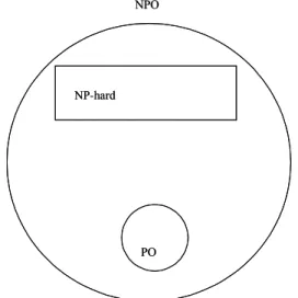
that if one of them is solved in polynomial time, so does the other one [3,7]. The optimization counterparts of NP, NP-complete and P are NPO, NP-hard and PO respectively. In other words (see Figure 2):
•NPO is the class of optimization problems whose
decision version is in NP;
•NP-hard is the class of optimization problems having
NP-complete decision counterparts;
•PO is the class of polynomial optimization problems, i.
e., the ones with polynomial decision versions.
APPROXIMATION, COMPLEXITY, OPTIMIZATION:
A 3-DIMENSIONAL MATCHING FULL OF INTEREST
by Vangelis Th. Paschos
EDITORIAL
Vangelis Th. Paschos Vangelis Th. Paschos Vangelis Th. Paschos Vangelis Th. Paschos NP NP-complete NP\P P NP NP-complete NP\P P2 AIROnews VIII, n.2 - Summer 2003
Formally, an NPO problem Π is defined as a quadruplet
(IΠ, SOLΠ, mΠ, optΠ), where:
• IΠ draws the set of instances of Π;
• SOLΠ(I) draws the set of feasible solutions of an
instance I ∈ IΠ;
• mΠ(I,S) is the measure of a solution S ∈ SOLΠ(I)
(the objective value of S);
• optΠ∈{min, max}.
Moreover, any I ∈ IΠ and S ∈ SOLΠ(I) are recognizable
in time polynomial in |I|, and, for any I ∈ IΠ and S
∈ SOLΠ(I), mΠ(I,S) is computable in time polynomial
in |I|. We will denote by optΠ(I) the optimal value (the
value of the optimal solution) of I and by ωΠ(I) the worst
value of I, i.e., the value of the worst feasible solution of
I. This solution can be defined [6,9] as the optimal
solution of the NPO problem Π′= (IΠ′, SOLΠ′, mΠ′,
optΠ′) where IΠ′= IΠ, SOLΠ′= SOLΠ and optΠ′ = max
if optΠ = min and optΠ′ = min if optΠ = max.
Since it is believed as very unlikely that a polynomial time algorithm could ever be devised to exactly solve Π, the area of polynomial approximation is interested in algorithms computing sub-optimal feasible solutions of
I in polynomial time. Such algorithms are called polynomial time approximation algorithms.
A given problem can admit several polynomial time approximation algorithms, each one providing a distinct feasible solution.
• How can we classify these algorithms with respect to their ability
in approximating the optimal solution of a generic instance I of the problem considered?"
• "How one can decide that an algorithm is better -- more
adapted -- than another one supposed to approximately solve the
same problem?"
To answer to the above questions, we need measures that count the "goodness" of an approximation algorithm A following some predefined criteria. The most common such criteria try to answer to one of the following questions (in what follows we consider Π fixed; so we simplify notations by eliminating it as index):
• Q1: by how m(I,S) differs from opt(I)?
• Q2: how many times is m(I,S) greater than (smaller than
when dealing with maximization problems) opt(I), in other words, what is the relative distance of m(I,S) from opt(I)?
• Q3: how m(I,S) is positioned with respect to opt(I) and
to ω(I), or more precisely, to what percentage of the best feasible values the value computed is lying?
Question Q1 induces the measure which in literature is called absolute performance guarantee; it is defined as ra(A,I) =
|m(I,S) - opt(I)|. Question Q2 induces the relative performance guarantee, or standard approximation ratio; it is
defined as r(A,I) = m(I,S)/opt(I). Finally, question Q3 induces the differential approximation ratio; it is defined as δ(A,I) = |ω(I) - m(I,S)|/ |ω(I) - opt(I)|. For more details about these ratios, the interested reader can be referred to ([2, 7, 8, 10, 11]).
With respect to any performance guarantee, one can partition the obtained results into three main categories: positive results:
here, one affirms that, for a given NP-hard problem, a given polynomial time approximation algorithm guarantees a performance measure bounded above (below when dealing with maximization problems) by a fixed constant;
negative results:
here, one affirms that, for a given NP-hard problem, no polynomial time approximation algorithm can guarantee a certain approximation level, unless an unlikely complexity theory condition (for example, P= NP) holds;
conditional results:
these results relate: either two types of approximation behavior of the same problem (see, for example, theorem 6.12 in [7] about MAX INDEPENDENT SET),
or the approximation behavior of a given NP-hard problem to the approximation behavior of another one.
EDITORIAL
Figure 2. The NPO-world as believed by researchers.
NPO NP-hard PO NPO NP-hard PO
3 AIROnews VIII, n.2 - Summer 2003
Results for the two last categories are, in fact, reductions preserving certain types of approximability properties of the problems involved.
Polynomial approximation has two main issues: one
operational and one structural. What is at operational stake,
is the fast and good solution of natural - real-world - problems, solution of which is a sine qua non condition in order that complex human systems can efficiently function. Let us think, for instance, to a company needing to plan for some hours later an urgent Hamiltonian tour on a hundred of sites. This can be seen as a version of the TRAVELINGSALESMAN exact solution
for which several days of computing time may be required even with the most modern computer systems. Therefore, such a way to apprehend the problem at hand is impossible. On the other hand, its apprehension by heuristics that do not guarantee always feasible solutions (and, furthermore, are probably not so fast) can be also unfeasible, even economically, or socially, or … dangerous. The use of polynomial time approximation for such problems, even if it does not guarantee computation of the best solution, it firstly guarantees solutions respecting all the constraints of the problem dealt and, moreover, these solutions are as near-optimal as possible.
The structural issue of polynomial approximation is even more interesting and challenging for a researcher. It allows the matching of complexity theory with combinatorial optimization and the mutual enrichment of both areas.
As in classical theory of algorithms, we can extend the classification of approximation algorithms to the classification of the problems solved by them. To be more precise, let us focus ourselves to the standard approximation ratio, denoted above by r, and consider a classification of approximation algorithms following the value of this ratio. Any such value induces what is commonly called approximation level. The most popular approximation levels are the following:
constant ratio: an algorithm is called constant-ratio algorithm when its approximation ratio r is a fixed constant, i.e., when its ratio does not depend on any parameter of the instance I;
polynomial time approximation schema: here we have a sequence of polynomial (in |I|) time algorithms receiving as inputs the instance I of an NP-hard problem and a fixed constant ε> 0; for any such є, they compute a feasible solution guaranteeing
approximation ratio 1+є (1-є when dealing with maximization problems);
fully polynomial time approximation schema: it is a polynomial time approximation schema but the complexity of any member of the sequence is polynomial both in |I| and 1/є;
logarithmic ratio: when the approximation ratio of the algorithm is O(log|I|);
polynomial ratio: when ∃є>0 such that the
approximation ratio achieved is (or when dealing with maximization problems).
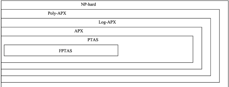
Classification of algorithms can be extended to classification of problems considering as approximation level of a problem the level of the best (known) approximation algorithm solving the problem under consideration. We so have the following most popular approximability classes:
APX: the class of NP-hard problems solved by constant-ratio polynomial time approximation algorithms;
PTAS: the class of NP-hard problems solved by polynomial time approximation schemata; FPTAS: the class of NP-hard problems solved by fully
polynomial time approximation schemata; Log-APX: the class of NP-hard problems solved by
polynomial time approximation algorithms achieving ratios logarithmic in |I|;
Poly-APX: the class of NP-hard problems solved by polynomial time approximation algorithms achieving ratios polynomial in |I|.
Figure 3 summarizes the discussion just above. Remark that since values for approximation ratios are in +,
there exists indeed a continuum of approximation classes. Note also that inclusions in Figure 3 are all strict. Relationships between complexity and approximation is even deeper since one can also prove completeness for some approximation classes. Recall that given a complexity class C and a reduction R, a problem Π is C-complete under reduction R if Π∈C and for any other problem Π′∈C, Π′ R-reduces to Π. Considering a complexity class, a complete problem for it can be thought as a hardest problem for the class under consideration. An easy way to think about completeness of Π is to say that Π is in C but not in a "superior" class (unless an unlikely complexity hypothesis holds). For example, Π is NP-complete means that it belongs to NP but not to P (unless P= NP). This can be extended for
EDITORIAL
( )
ε4 AIROnews VIII, n.2 - Summer 2003
approximability classes. For an approximability class C
(recall that such a class, e.g. APX, is the set of problems
approximable within approximation ratios the value of which correspond to a certain level, e.g. fixed constant ratios) a problem is C-complete (e.g., APX-complete) if it belongs to C (e.g., APX) but it cannot belong to a "superior" approximability class (e.g., PTAS) unless an unlikely complexity condition holds (e.g., P= NP). Note finally that the class of problems solved by fully polynomial time approximation schemata (FPTAS when dealing with standard approximation), considered as the highest approximability class, cannot have complete problems since the only higher approximation level is class PO (that can be considered as the class of
problems polynomially solved within approximation ratio 1). For more details about structure in standard approximation classes, the interested reader can be referred to [3, 5], while, for the differential ones, to [1].
Vangelis Th. Paschos LAMSADE, Université Paris-Dauphine Place du Maréchal De Lattre de Tassigny,
75775 Paris Cedex 16, France [email protected]
[1] G. Ausiello, C. Bazgan, M. Demange, and V. Th. Paschos. Completeness in differential approximation classes. Cahier du LAMSADE 204, LAMSADE, Université Paris-Dauphine, 2003. Available on http://www.lamsade.dauphine.fr/cahiers.html. [2] G. Ausiello, P. Crescenzi, G. Gambosi, V. Kann, A. Marchetti-Spaccamela, and M. Protasi, “Complexity and approximation. Combinatorial optimization problems and their approximability properties”, Springer, Berlin, 1999.
[3] G. Ausiello, P. Crescenzi, and M. Protasi, Approximate solutions of NP optimization problems, Theoret. Comput. Sci., 150:1-55, 1995.
[4] S. A. Cook, The complexity of theorem-proving procedures. In Proc. STOC'71, 151-158, 1971.
[5] P. Crescenzi and A. Panconesi, Completeness in approximation classes, Inform. and Comput, 93(2):241-262, 1991.
[6] M. Demange and V. Th. Paschos, On an approximation measure founded on the links between optimization and
polynomial approximation theory, Theoret. Comput. Sci., 158:117-141, 1996.
[7] M. R. Garey and D. S. Johnson, “Computers and intractability. A guide to the theory of NP-completeness”, H. Freeman, San Francisco, 1979.
[8] D. S. Hochbaum, editor. “Approximation algorithms for NP-hard problems”, PWS, Boston, 1997.
[9] Monnot, V. Th. Paschos, and S. Toulouse, Differential approximation results for the traveling salesman problem with distances 1 and 2, European J. Oper. Res., 145(3):557--568, 2002
[10] J. Monnot, V. Th. Paschos, and S. Toulouse, “Approximation polynomiale des problèmes NP-difficiles: optima locaux et rapport différentiel”, Informatique et Systèmes d'Information, Hermès, Paris, 2003
[11] C. H. Papadimitriou and K. Steiglitz, “Combinatorial optimization: algorithms and complexity”, Prentice Hall, New Jersey, 1981. References