Negotiation Can be as Hard as Planning: Deciding
Reachability Properties of Distributed Negotiation Schemes
Paul E. Dunne [email protected]
Department of Computer Science, University of Liverpool, Liverpool L69 7ZF, UK
Yann Chevaleyre [email protected]
LAMSADE, University of Paris-Dauphine, 75775 Paris Cedex 16, France
Abstract
Distributed negotiation schemes offer one approach to agreeing an allocation of re-sources among a set of individual agents. Such schemes attempt to agree a distribution via a sequence of locally agreed ‘deals’ – reallocations of resources among the agents – ending when the result satisfies some accepted criteria. Our aim in this article is to demon-strate that some natural decision questions arising in such settings can be computationally significantly harder than questions related to optimal clearing strategies in combinatorial auctions. In particular we prove that the problem of deciding whether it is possible to progress from a given initial allocation to some desired final allocation via a sequence of “rational” steps is pspace-complete.
1. Introduction
The abstraction wherein a triple hA, R, U i represents sets of agents, resources, and “utility” functions by which individual agents associate values with resource subsets, has proven to be a useful mechanism in which to consider problems concerning how best to distribute a finite collection of items among a group of agents. In very informal terms, two general approaches have been the basis of algorithmic studies concerning how to organise the allocation of resources to agents: centralized mechanisms of which combinatorial auction techniques are possibly the best-known exemplar; and distributed methods deriving from the contract-net model formulated in (Smith, 1980) whose properties are the subject of the present article. In Combinatorial Auction schemes, e.g. (Sandholm, 2002; Sandholm & Suri, 2003; Tennenholz, 2000; Yokoo et al., 2004; Parkes & Ungar, 2000a, 2000b), a centralized controlling agent (the “auctioneer”) assumes responsibility for determining which agents receive which resources basing its decisions on the bids submitted by individual agents. Bidding protocols vary in expressive complexity from those that simply allow an agent to submit a single bid of the form hS, pi expressing the fact that the agent is prepared to pay some price p in return for the subset S of R to methods allowing a number of different subsets to be described in separate bids, e.g. the so-called xor language discussed in (Sandholm, 2002). A typical aim of the auctioneer is to decide which bids to accept so as to maximise the overall price paid subject to at most one agent being granted any resource. This scheme gives rise to the Winner Determination Problem of deciding which bids among those submitted are successful. In its most general form Winner Determination is np–hard, but there are
a number of powerful heuristic approaches and winner determination can be efficiently carried out albeit if the bidding language is of very limited expressiveness. Despite the practical effectiveness of these approaches, there has, however, been a recent revival of interest in autonomous distributed negotiation schemes building on the pioneering study of these by Sandholm (1998). It is not difficult to identify motivations underpinning this renewed interest: the implementation overheads in schema where significant numbers of bids (possibly having complex structures) are communicated to a single controlling agent; the potential difficulties that might arise in persuading an individual agent to assume the rˆole and responsibilities of auctioneer; similarly the need to ensure that bidding agents comply with the decisions made by the auctioneer; the issues raised in deciding on a bidding protocol given the extremes from languages that are highly expressive but computationally hard for winner determination to highly rigid and simple bidding languages which, while tractable, face the problem of no allocation at all being compatible with the bids received; finally, aside from the computational problems with which the auctioneer is faced, there is the highly non-trivial issue for the agents bidding as regards selecting and pricing resource sets so as to optimise the likelihood of their “most preferred” bid being accepted.
Faced with such computational issues, notwithstanding the advances in combinatorial auction technology, environments whereby allocations are settled following a process of local improvements negotiated by agents agreeing changes, appear attractive, particularly if the protocols for proposing and implementing resource transfers between agents limit the number of possibilities that individual agents may have to review.
The principal results of this paper establish that, far from resulting in a computationally more tractable regime or, indeed, even one that exhibits complexity “no worse” than the np-hard status of winner determination, a number of natural decision questions concerning simple distributed negotiation protocols, have significantly greater complexity. In particu-lar, we show that given a description of a resource allocation setting – hA, R, U i – together with some initial and desired allocations hP(s), P(t)i deciding if the desired allocation can
be realised by a sequence of rational “local” reallocations is pspace-complete. Thus, de-ciding if a particular type of negotiation will be effective in bringing about a reallocation is at a similar level of complexity to classical A.I. planning problems, e.g. as considered in the work of (Bylander, 1994). We, further, note one of our results resolves a question left open from (Dunne et al., 2005): specifically we show the problem of deciding if there is a rational sequence of “one-resource-at-a-time” reallocations to progress between given start-ing and final allocations, to be pspace–complete, improvstart-ing upon the earlier np-hardness classification.
In the next section we introduce the formal structures of contract-net derived distributed negotiation reviewing the components of this presented by Sandholm (1998) together with terminology and notation that will be used subsequently. Section 3 describes the decision questions that are considered, summarises related work concerning these, and presents a formal statement of the results subsequently proved in Section 5. Separating these two sections, we give a high-level, informal overview of the proof mechanisms in Section 4.
The problems analysed in Section 5 are concerned with what might be called “local” properties of a given allocation setting, specifically whether it is possible to progress from a given starting point to a desired allocation via a restricted class of negotiation primitives. In Section 6 we address “global” properties of such schemes which we term Convergence
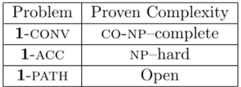
and Accessibility. Convergence addresses a property of resource allocation settings that has been studied earlier in work of (Endriss & Maudet, 2004; Chevaleyre et al., 2005), namely whether a setting is such that using a restricted class of deals, no matter what starting allocation is in force and which ever sequence of allowed rational deals is employed, the outcome will always be some optimal allocation. Perhaps suprisingly, for the restricted deal classes under which the questions considered in Section 5 turn out to be pspace–complete, deciding convergence properties is “only” coNP–complete. Accessibility, considers whether from a given starting point it is possible to reach an optimal outcome: this, too, turns out to be pspace–complete. We present concluding comments and discuss further developments in Section 7.
2. Resource Allocation Settings and Local Negotiation
The principal structure we consider in this paper is presented in the following definition.
Definition 1 A resource allocation setting is defined by a triple hA, R, U i where
A = {A1, A2, . . . , An} ; R = {r1, r2, . . . , rm}
are, respectively, a set of (at least two) agents and a collection of (non-shareable) resources. A utility function, u, is a mapping from subsets of R to rational values. Each agent Ai∈ A
has associated with it a particular utility function ui, so that U is hu1, u2, . . . , uni. An
allocation P of R to A is a partition hP1, P2, . . . , Pni of R. The value ui(Pi) is called the
utility of the resources assigned to Ai. We use Πn,m to denote the set of all partitions of m
resources among n agents: it is easy to see that |Πn,m| = nm, there being n different choices
for the owner of each of the m resources.
Given some starting allocation, P ∈ Πn,m, individual agents may wish to “improve” this: for
the purposes of this paper, the concept of an allocation Q improving upon an allocation P will be defined in purely quantitative terms. Even within these limits there are, of course, many different methods by which an allocation P may be quantitatively rated. For the settings we consider we concentrate on the measure of utilitarian social welfare, denoted σu(P ), which is simply the sum of the agents’ utility functions for their allocated resources
under P , i.e. σu(P ) =Pni=1 ui(Pi).
We next formalise the concepts of deal and contract path.
Definition 2 Let hA, R, U i be a resource allocation setting. A deal is a pair hP, Qi where P = hP1, . . . , Pni and Q = hQ1, . . . , Qni are distinct partitions of R. The effect of
imple-menting the deal hP, Qi is that the allocation of resources specified by P is replaced with that specified by Q. For a deal δ = hP, Qi, we use Aδ to indicate the subset of A involved, i.e. Ak∈ Aδ if and only if Pk 6= Qk.
Let δ = hP, Qi be a deal. A contract path for δ is a sequence of allocations
∆ = hP(0) ; P(1) ; . . . ; P(d−1) ; P(d)i
in which P = P(0) and P(d) = Q. The length of ∆, denoted |∆| is d, i.e. the number of deals in ∆.
Sandholm (1998) presents a number of restrictions on the form that deals may take, one motivation for such being to limit the number of deals that a single agent may have to consider. The class of restricted deals presented in the following definition includes those analysed in (Sandholm, 1998).
Definition 3 Let δ = hP, Qi be a deal involving a reallocation of R among A.
a. δ is bilateral if |A|δ = 2.
b. δ is t-bounded if δ is bilateral and the number of resources whose ownership changes after implementing δ is at most t.
c. δ is a t-swap if δ is bilateral and for some s ≤ t, Q is formed by exactly s resources in Pi being assigned to Aj and replaced, in turn, by exactly s resources of Pj.
The class of t-bounded and t-swap deals are simple extensions of the classes of O-contracts and S-contracts in (Sandholm, 1998): O-contracts being 1-bounded deals and, similarly, S-contracts are 1-swap deals. We note that t-swap deals are a special case of (2t)-bounded deals.
We introduce the concept of a deal being rational in the following definition. It will be useful to consider two forms: one linked to the particular quantitative measure of utilitarian social welfare; and, more generally, one which is expressed in terms of arbitrary quantitative measures.
Definition 4 A deal hP, Qi is individually rational (ir) if and only if σu(Q) > σu(P ). For
hA, Ri as before, an evaluation measure is a (total) mapping σ : Πn,m → Q. A deal hP, Qi
is σ-rational if and only if σ(Q) > σ(P ).
We note that δ is individually rational if and only if δ is σu-rational. Where there is no
ambiguity we will simply refer to a deal being rational without specifying σ.
The notions of rationality introduced above are now extended in order to introduce the structures that form the main object of study in this paper: σ-rational paths.
Definition 5 For hA, Ri and an evaluation measure, σ, a sequence of allocations
∆ = hP(0) ; P(1) ; . . . ; P(d)i
is a σ-rational contract path for the (σ-rational) deal hP(0), P(d)i if for all 1 ≤ i ≤ d,
hP(i−1), P(i)i is σ-rational.
More generally, if Φ : Πn,m× Πn,m→ {>, ⊥}, is some predicate on deals, we say that
∆ is a Φ-path if Φ(P(i−1), P(i)) holds for each 1 ≤ i ≤ d. We say that Φ-deals are complete for σ-rationality if
3. Decision Problems in Localised Negotiation
The ideas introduced in Definitions 3 and 4 combine to focus on deals that not only restrict their structure (in the sense of limiting the number of agents and the number of resources involved) but also add the further condition that a deal must result in a better allocation. It is as a result of such rationality conditions that significant difficulties arise within local negotiation approaches. Thus, two extremes are already apparent in the following result from (Sandholm, 1998).
Fact 1
a. 1-bounded deals are complete for σ-rationality.
b. ir 1-bounded deals are not complete for individual rationality.
c. If |A| ≥ 3, then ir bilateral deals are not complete for individual rationality. Among the questions that naturally follow from Fact 1 are those listed below:
Q1. Are there “reasonable” conditions that can be imposed on collections of utility func-tions, U , so that in settings hA, R, U i where these hold, ir 1-bounded deals are com-plete for individual rationality?
Q2. Given hhA, R, U i, P(s), P(t)i with hP(s), P(t)i being ir, how efficiently can one
deter-mine whether there is a rational 1-bounded contract path for hP(s), P(t)i?
Q3. When such a path does exist what can be proven regarding its properties, e.g. number of deals involved, etc.?
The first has been considered in (Endriss & Maudet, 2004; Chevaleyre et al., 2005) and while these offer some positive results, the initial analyses regarding the other two questions presented in (Dunne, 2005; Dunne et al., 2005) are rather less encouraging.
Fact 2
a. Given hhA, R, U i, P(s), P(t)i with hP(s), P(t)i being ir, the problem of deciding if there
is a rational 1-bounded contract path for hP(s), P(t)i is np–hard. (Dunne et al., 2005, Thm. 12)
b. For every m = |R| ≥ 7 there are choices of hhA, R, U i, P(s), P(t)i for which: there is a unique ir 1-bounded contract path, ∆, for the ir deal hP(s), P(t)i and |∆| = Ω(2m).
(Dunne, 2005, Thm. 3).
c. For every m = |R| ≥ 6 there are choices of hhA, R, U i, P(s), P(t)i with |A| = 3 and
for which: there is a unique ir bilateral contract path, ∆, for the ir deal hP(s), P(t)i and |∆| = Ω(2m/3). (Dunne, 2005, Thm. 6).
Although the analysis leading to the proof of Fact 2(a) is couched in terms of ir 1-bounded deals, it is straightforward to adapt it to establish np-hardness for ir 1-swap deals. The principal contribution of the present article is in obtaining tight complexity classifications for these decision problems: Theorem 4 proving both to be pspace–complete.
We consider two general forms of decision problems in Section 5 where Φ in the descrip-tion below is a predicate on deals.
Φ − PATHE
Instance: hhA, Ri, σ, P(s), P(t)i with σ(P(t)) > σ(P(s)).
Question: Is there a Φ-path ∆ for the deal hP(s), P(t)i? Φ − PATHU
Instance: hhA, R, U i, P(s), P(t)i with σu(P(t)) > σu(P(s)).
Question: Is there a Φ-path ∆ for the deal hP(s), P(t)i?
Although, superficially, these are similar problems, the significant distinction that should be noted is that Φ − PATHU is a restricted special case of Φ − PATHE. We elaborate further on the differences in our overview of Section 4.
The particular instantiations of Φ that we consider are given below where m = |R|. It is convenient to introduce distinct names for the relevant decision problem induced.
1. Φ(P, Q) holds if and only if hP, Qi is a σ-rational 1-bounded deal. Subsequently denoted 1-path as the resulting specialisation of Φ − PATHE.
2. Φ(P, Q) holds if and only if hP, Qi is an ir 1-swap deal. This being denoted 1-swap for the corresponding instantiation of Φ − PATHU.
3. Φ(P, Q) holds if and only if hP, Qi is an ir 1-bounded deal. We denote this special case of Φ − PATHU by iro-path.
We will show that each of the resulting decision problems is pspace-complete. 4. Overview of Proof Methods
This section has three aims: firstly, to address the technical question of how instances of the decision problems introduced at the conclusion of Section 3 are encoded; secondly, to elaborate on the differences between the forms Φ − PATHE and Φ − PATHU; and, finally, to outline the organisation and structure of the proofs presented in Section 5.
4.1 Representing Instances
In order to describe instances of Φ − PATHE or Φ − PATHU the problem of encoding functions whose domain is exponentially large in |R|, i.e. σ : Πn,m → Q; ui : 2R → Q
must be addressed. Of course, one approach would be simply to enumerate values using some ordering of the relevant domain. There are, however, at least two objections that can be made to such solutions: since the domains are exponentially large – nm and 2m
– exhaustive enumeration would in practical terms be infeasible even in the case of very simple functions, e.g. u(S) = 1 if |S| is even; u(S) = 2 otherwise. The second objection is that exhaustive enumeration schemes are liable to give misleading assessments of run-time complexity: an algorithm that is polynomial-time in the length of such an encoding, is actually of exponential complexity in terms of the numbers of agents and resources.
In (Dunne et al., 2005) the following desiderata are proposed for encoding a utility function, u, as a sequence of bits ρ(u):
a. ρ(u) is ‘concise’ in the sense that the length, e.g. number of bits, used by ρ(u) to describe the utility function u within an instance is “comparable” with the time taken by an optimal program that computes the value of u(S).
b. ρ(u) is ‘verifiable’, i.e. given some binary word, w, there is an efficient algorithm that can check whether w corresponds to ρ(u) for some u.
c. ρ(u) is ‘effective’, i.e. given S ⊆ R, the value u(S) can be efficiently computed from the description ρ(u).
It is, in fact, possible to identify a representation form that satisfies all three of these criteria: we represent each member of U in a manner that does not require explicit enumeration of each subset of R and allows (a) to be met; uses a ‘program’ form whose syntactic correctness can be efficiently verified, hence satisfying (b); and for which termination in time linear in the program length is guaranteed, so meeting the condition set by (c). The class of programs employed are the so-called straight-line programs (slp) which have a natural correspondence with combinational logic networks (Dunne, 1988).
Definition 6 An (m, s)-combinational network C is a directed acylic graph in which there are m input nodes, Zm, labelled hz1, z2, . . . , zmi all of which have in-degree 0. In addition, C
has s output nodes, called the result vector. These are labelled hts−1, ts−2, . . . , t0i, and have
out-degree 0. Every other node of C has in-degree at most 2 and out-degree at least 1. Each non-input node (gate) is associated with a Boolean operation of at most two arguments.1 We use |C| to denote the number of gate nodes in C. Any Boolean instantiation of the input nodes to a ∈ h0, 1im naturally induces a Boolean value at each gate of C: if h is a
gate associated with the operation θ, and hg1, hi, hg2, hi are edges of C then the value h(a) is
g1(a)θg2(a). Hence a induces some s-tuple hts−1(a), . . . , t0(a)i ∈ h0, 1is at the result vector.
For the (m, s)-combinational network C and a∈ h0, 1im, this s-tuple is denoted by C(a).
Although often considered as a model of parallel computation, (m, s)-combinational net-works yield a simple form of sequential program – straight-line programs – as follows. Let C be an (m, s)-combinational network to be transformed to a straight-line program, slp(C), that will contain exactly m + |C| lines. Since C is directed and acyclic it may be topolog-ically sorted, i.e. each gate, g, given a unique integer label τ (g) with 1 ≤ τ (g) ≤ |C| so that if hg, hi is an edge of C then τ (g) < τ (h). The line li of slp(C) evaluates the input
zi if 1 ≤ i ≤ m and the gate for which τ (g) = i − m if i > m. The gate labelling means
that when g with inputs g1 and g2 is evaluated at lm+τ (g) since gi is either an input node
or another gate its value will have been determined at lj with j < m + τ (g).
Definition 7 Let R be as previously with |R| = m, and u a mapping from subsets of R to whole numbers, i.e. a utility function. The (m, s)-network Cu is said to realise the utility function u if: for every S ⊆ R with s the instantiation of Zm given by zi = 1 if and only if
ri ∈ S, it holds
u(S) = val(C(s))
1. In practice, we can restrict the Boolean operations employed to those of binary conjunction (∧), binary disjunction (∨) and unary negation (¬).
where for b = hbs−1, bs−2, . . . , b0i ∈ h0, 1is, val(b) is the whole number whose s-bit binary
expansion is b, i.e. val(b) =Ps−1
i=0bi∗ 2i, where bi is treated as the appropriate integer value
from {0, 1}.
Definition 7 provides a method of encoding utility functions u : 2R → N ∪ {0} in instances of Φ − PATHU: each ui ∈ U is represented by a straight-line program, slp(Cui)
derived from a suitable combinational network. For instances of Φ − PATHE, the function σ : Πn,m → N ∪ {0} can be encoded in a similar fashion. For example, via a (mn, s +
1)-combinational network, C, whose input zi,j indicates if rj ∈ Pi; val(C(α)) is again an s-bit
value: the additional output bit being used to flag if the instantiation α is not a valid partition, e.g. if zi,j = 1 and zk,j= 1 for some rj and i 6= k.2
A key property of encodings via slps is the following result of (Fischer & Pippenger, 1979; Schnorr, 1976)
Fact 3 If f : {0, 1}m → {0, 1}s is computable by a deterministic Turing Machine program
in time T , then f may be realised by an slp containing O(T log T ) lines.
It should be noted that the proof of Fact 3 is constructive, i.e. the translation is not merely an existence argument and, in addition, a suitable slp can be built in time polynomial in T . Thus a further consequence is our subsequent reductions do not need to give explicit detailed constructions of slps.3 It will suffice to specify σ or U for it to be apparent that these may be computed efficiently: Fact 3 then ensures suitable representations can be formed.
4.2 Distinctions between Φ − PATHE and Φ − PATHU
We recall that Φ − PATHE concerns the existence of σ-rational Φ-paths with the evalua-tion measure, σ, forming part of the instance whereas Φ − PATHU focuses on the partic-ular choice σ = σu with the collection of utility functions forming part of the instance.
Given that our primary interest is in the measure σu, it may seem that there is some
redundancy in considering Φ − PATHE, e.g. if we introduce utility functions for which u2 = u3 = . . . un = 0, defining u1(S) as σ(hS, P2, P3, . . . , Pni), where Pi is the
particular subset of R held by Ai in a specific case of A1 holding S, then one has σu(P )
(in the “new” setting) equal to σ(P ) (in the original form). The main objection to such an approach is that the utility function, u1, is likely to have allocative externalities, i.e.
its value is dependent not only on the actual resources held by A1 but also upon how the
other resources are distributed. It has tended to be the normal assumption, often not even mentioned directly,4that utility functions do not have such externalities, e.g. (Dunne, 2005; Dunne et al., 2005; Endriss et al., 2003; Sandholm, 1998). While the complexity classifi-cation of Φ − PATHE has some interest in itself, our main concern is with the decision
2. Although we describe the range of σ and u to be whole numbers using slp encodings, it is a trivial matter to extend to integers, e.g. use an additional output bit to indicate whether a value is positive or negative; and to rationals, e.g. treat one section of the output bits as defining a numerator, the remaining section as a denominator.
3. Some illustrative constructions of slps in specific polynomial-time reductions are presented in (Dunne et al., 2005, pp. 33–4).
4. One of the few exceptions is (Yokoo et al., 2004) which explicitly states that the valuation functions considered are assumed to be free of allocative externalities.
problem relating to Φ − PATHU, which focuses on a single measure of how good an allo-cation is – σu – and, in keeping with standard approaches, assumes utility functions to be
free from externalities.
One point of some importance in our proofs concerning the variant of Φ − PATHEgiven in Section 5, is that the evaluation measure, σ, constructed in the instance hA, R, σ, P(s), P(t)i does not admit a direct translation to hA, R, U , P(s), P(t)i in which U is externality-free and is such that σu(P ) = σ(P ). We introduce a “coding trick” by means of which a general
translation from any hA, R, σi to a setting h{A1, A2}, R0, {u1, u2}i results. In particular this
translation provides the means by which two special cases of Φ − PATHU can be proven pspace-hard, i.e. the problems 1-swap and iro-path.
Of course, in principle, our proofs that the special cases of Φ − PATHU are pspace-hard could be presented directly, i.e. without reference to Φ − PATHE and the coding device used. There are, however, a number of reasons why we avoid such an approach. The first of these is the technical complexity of the proofs themselves: although the translation from Φ − PATHE to Φ − PATHU turns out to be relatively straightforward, the central result that 1-path is pspace–hard on which our subsequent classifications build, is rather more involved. We note that notwithstanding the use of arbitrary evaluation measures, the problem 1-path is a “natural” decision question whose properties, we contend, merit consideration in their own right.
4.3 Proof Structure
We begin by recalling the decision problems considered.
1-path (special case of Φ − PATHE)
Instance: hA, R, σ, P(s), P(t)i with σ(P(t)) > σ(P(s)).
Question: Is there a σ-rational 1-bounded path for hP(s), P(t)i?
1-swap (special case of Φ − PATHU)
Instance: hA, R, U , P(s), P(t)i with σu(P(t)) > σu(P(s)).
Question: Is there an ir 1-swap path for hP(s), P(t)i? iro-path (special case of Φ − PATHU)
Instance: hA, R, U , P(s), P(t)i with σu(P(t)) > σu(P(s)).
Question: Is there an ir 1-bounded path for hP(s), P(t)i?
Subject to Φ(P, Q) being decidable in pspace it is straightforward to show that Φ − PATHE∈ pspace. For each of the problems listed, the corresponding Φ(P, Q) is decidable in (deterministic) polynomial-time.
On first inspection the approach taken to proving pspace–hardness may seen rather indirect: an “auxiliary problem” – Achievable Circuit Sequence (acs) – is defined inde-pendently of the arena of multiagent negotiation contexts, with the assertion “1-path is pspace-complete”, justified by showing “acs is pspace-complete” (Theorem 2) and then acs ≤p 1-path (Theorem 3). This auxiliary problem has, however, two important
reduction techniques.5 The second property of acs is that its formal structure is very similar to that of 1-path.
Thus, acs is concerned with deciding a property of a given (N, N )-combinational logic network, C, with respect to two distinct binary N -tuples. The N inputs of C are inter-preted as a sequence of n data bits hx1, x2, . . . , xni coupled with a sequence of m value
bits hy0, y1, . . . , ym−1i; the N outputs are viewed in a similar fashion. Now, suppose that
a = hdata(a), value(a)i and b = hdata(b), value(b)i are the binary N -tuples given with C to form an instance of acs.
Recall that val(y) is the whole number represented by the m value bits of C, i.e. val(y) = Pm−1
i=0 (2i) ∗ yi, and define
hdatak(a), valuek(a)i = (
hdata(a), value(a)i if k = 0 C(hdatak−1(a), valuek−1(a)i) if k > 0
Since the output of any (N, N )-combinational logic network on a given instantiation of its inputs is uniquely determined, the sequence [hdatak(a), valuek(a)i]k≥0 is well-defined and
unique.
Informally, acs asks of its instance hC, a, bi if there is some value t ≥ 1 with which: a. hdatat(a), valuet(a)i = hdata(b), value(b)i
b. For each 1 ≤ i ≤ t, val(valuei(a)) > val(valuei−1(a)).
Although the formal technical argument that acs ≤p 1-path given in Section 5.2 involves
a number of notational complexities, its basic strategy is not difficult to describe. Recalling that an instance of acs consists of an (n + m, n + m)-combinational logic network, C, together with instantiations hx, yi, hz, wi from h0, 1in+m, the instance hAC, RC, σ, P(s), P(t)i
of 1-path that is formed uses 5 agents. The resource set RC contains disjoint sets each of
size 2(n + m) – RV and RW – with “appropriate” subsets of RX (for X ∈ {V, W }) mapping to elements of h0, 1in+m. In the initial allocation, P(s), A1 holds the subset of RV and the
subset of RW that maps to hx, yi ∈ h0, 1in+m. In the final allocation, P(t), A1 should hold
the subsets of RV and RW that map to hz, wi. For the agents A2 and A3: the former
should hold subsets of RV while the latter holds subsets of RW. The evaluation measure, σ, is constructed so that any allocation, Q, for which Q2 6⊆ RV or Q36⊆ RW has σ(Q) < 0.
The main idea is to simulate the witnessing sequence {hxi, yii}0≤i≤t for a positive in-stance of acs by a sequence of allocations to A1, i.e. from the initial allocation to A1
which we recall mapped to hx0, y0i ∈ h0, 1in+m subsequent allocations to A
1 will be those
subsets of RV and RW which map to hx
i, yii ∈ h0, 1in+m. The problem that arises in this
simulation is that if Q(i) is the allocation in which A1’s holding reflects hxi, yii then the
deal hQ(i), Q(i+1)i although σ-rational for the evaluation measure constructed, will not be 1-bounded. In order to effect this deal, a sequence of 1-bounded σ-rational deals is used which involve the following stages:
1. a subset of RV is transferred one resource at a time from A2 to A4;
5. That is to say, “easy” pace the notational overheads inherent in most generic simulations of resource-bounded Turing machine classes: the elegant casting of Turing machine behaviour in terms of planning operators presented in (Bylander, 1994) being a notable exception.
2. a subset of RV is transferred one resource at a time from A1 to A2
3. the resources moved into A4 in stage (1) are transferred to A1.
The subset of RV held by A1 on completion will map to hxi+1, yi+1i, while the subset
of RW continues to map to hxi, yii. These three stages are then repeated, but now with
resources from RW and the agent A3 involved, so that the subset of RW held by A1 will,
on completion, map to hxi+1, yi+1i.
In order to track whether resources should be moved out of A4 into A1, a “marker”
resource, µ, initially held by A5 is used: µ is reallocated to A4 at the end of the second
phase and returned to A5 once the third stage is complete.
The notational overhead in the proof stems from specifying the evaluation measure, σ, in such a way that a σ-rational 1-bounded sequence of deals to go from P(s) to P(t) is possible if and only the source instance of acs should be accepted.
5. PSPACE-complete Negotiation Questions
We begin with the relatively straightforward proof that the decision problems we consider are all decidable by pspace algorithms. Since all of these are specialisations of Φ − PATHE and the predicate Φ(P, Q) is polynomial-time decidable for each, it suffices to prove,
Theorem 1 For predicates Φ : Πn,m×Πn,m→ {>, ⊥} such that Φ(P, Q) is polynomial-time
decidable, Φ − PATHE∈ pspace.
Proof. Given an instance hA, R, σ, P(s), P(t)i of Φ − PATHE in which σ : Π
n,m → Q is
described in the form of a straight-line program, use a non-deterministic algorithm which proceeds as follows:
P := P(s) loop
Non-deterministically choose an allocation Q ∈ Πn,m
if ¬Φ(P, Q) then reject else if Q = P(t) then accept else P := Q
end loop
If a Φ-path realising hP(s), P(t)i exists then this non-deterministic algorithm has a compu-tation that will successfully identify it. The algorithm need only record the allocations P and Q occurring in the loop body and thus can be implemented in npspace. The theorem now follows from Savitch’s Theorem: npspace=pspace, (Savitch, 1970). 2
5.1 The Achievable Circuit Sequence Problem (acs)
The following decision problem is central to our subsequent argument. Achievable Circuit Sequence (acs)
n + m outputs, hZn, Wmi; hx, yi, hz, wi ∈ h0, 1in+m.
Question: Is there a sequence
Γ = hhx0, y0i, hx1, y1i, . . . , hxk, ykii
such that
a. hx0, y0i = hx, yi,
b. hxk, yki = hz, wi,
c. ∀ 1 ≤ i ≤ k, C(xi−1, yi−1) = hxi, yii and val(y
i) > val(yi−1)?
Before showing that acs is pspace-complete, we present a small example instance. This example will be used subsequently to illustrate the proof that acs≤p1-path.
Example 1 The table below describes (in truth-table form) the input and output charac-teristics of a (4, 4)-combinational logic network, C:
x1 x2 y1 y2 z1 z2 w1 w2 val(hy1, y2i) val(hw1, w2i)
0 0 0 0 0 0 0 1 0 1
0 0 0 1 0 1 1 0 1 2
0 1 1 0 1 1 1 1 2 3
1 1 1 1 1 1 1 1 3 3
Table 1: Example Function for instance of acs
[The twelve unspecified entries for hx1, x2, y1, y2i all produce h0000i as their output.]
The instance hC, h0000i, h1111ii of acs is accepted, as witnessed by the sequence h0000i ; h0001i ; h0110i ; h1111i
In contrast the instance hC, h0000i, h1011ii is rejected: the unique continuation of h0000i never reaches h1011i.
Theorem 2 acs is pspace-complete.
Proof. An instance hC, x, y, z, wi of acs can be decided by a (deterministic) polynomial-space computation that iterates evaluating
hxi+1, yi+1i = C(xi, yi)
(starting with hx, yi).
This computation terminates either when val(yi+1) ≤ val(yi) (the instance is rejected) or when hz, wi occurs with the former condition taking precedence when hxi+1, yi+1i = hz, wi. Since there are only 2n+m possible cases, eventually one of these two termination
conditions must arise. The whole computation can be accomplished in polynomial-space since only the current hxi, yii need be remembered.
For pspace–hardness we use a generic reduction, i.e. given a Turing machine program, M , input s, and space-bound S = |s|c we form an instance of acs that is accepted if and only if s is accepted by M within an S-space bounded computation. We may assume that M has a unique accepting configuration u. It suffices to note that from the description of M we can build a (t, t)-combinational logic network CM whose input bits encode configurations
of M on exactly S tape-cells. For such a configuration, χ, CM(χ) = π if and only if the
configuration π follows in exactly one move of M from the configuration χ. Note we may use the convention that CM(u) = u for the unique accepting configuration. Combine CM
with a p-bit counter, D, i.e. val(D(v)) = val(v) + 1 with p chosen large enough so that the total number of configurations of S-tape bounded configurations of M can be represented in p bits.6 Now let s be the instantiation of the inputs of CM corresponding to the initial
configuration of M on input s: s is accepted by M if and only if h(CM, D), hs, 0pi, hu, 1pii
is accepted as an instance of acs. 2
5.2 acs is polynomially-reducible to 1-path
It will be convenient to introduce the following notation and definitions.
For V = {v1, v2, . . . , vn+m} and W = {w1, w2, . . . , wn+m} disjoint sets of n + m
propo-sitional variables, we define sets RV = {v
1, v2 , . . . , vn+m, ¬v1 , . . . , ¬vn+m}
RW = {w
1, w2 , . . . , wn+m, ¬w1 , . . . , ¬wn+m}
R = RV ∪ RW
In our subsequent notation, in order to avoid repetition, X refers to either of V or W . Given S ⊆ R, the subset SX is defined via SX = S ∩ RX. We define a partial mapping, β : 2R→ h0, 1in+m as follows.
For all of the cases below, β(S) is undefined, i.e. β(S) = ⊥ whenever SV 6= ∅ and SW 6= ∅ or S ⊆ RX and |S| 6= n + m or
S ⊆ RX and there is some i for which {xi, ¬xi} ⊂ S
For the remaining cases,
β(S) = ha1a2. . . an+mi where ai = (
0 if ¬xi ∈ S
1 if xi ∈ S
Given a = ha1a2. . . an+mi ∈ h0, 1in+m, there is a uniquely defined set S ⊆ RX for which
β(S) = a. Thus we can introduce β−1X as a total mapping from h0, 1in+m to subsets from RX, as
βX−1(a) = S ⊆ RX such that β(S) = a
For a ∈ h0, 1in+m, we denote by valm(a) the whole number whose m bit binary
representa-tion is an+1an+2· · · an+m, i.e the valuePn+mi=n+1 (ai) ∗ 2n+m−i.
Let S and T be subsets of RX that satisfy all the conditions (CS1)–(CS4) below.
CS1. S ∩ T = ∅
CS2. For each i (1 ≤ i ≤ n + m) either xi 6∈ S or ¬xi6∈ S
CS3. For each i (1 ≤ i ≤ n + m) either xi 6∈ T or ¬xi6∈ T
CS4. For each i (1 ≤ i ≤ n + m) if (xi 6∈ S) and (¬xi 6∈ S) then (xi ∈ T ) or (¬xi ∈ T )
For such sets S, T the composite set, S ⊗ T , is the subset of RX given by
S ⊗ T = S \ ({ x : ¬x ∈ T } ∪ { ¬x : x ∈ T }) [ T
Now suppose that C is an (N, N )-combinational logic network with N = n + m, a ∈ h0, 1in+m, and S ⊆ RX, is such that for each i, either x
i 6∈ S or ¬xi 6∈ S. The difference
set for S with respect to a is the subset of RX,
diffX(S, a) = βX−1(a) \ S
The following lemma establishes some useful relationships between the composite set oper-ation, ⊗, and difference sets.
Lemma 1 Let C be an (n + m, n + m)-combinational logic network, a ∈ h0, 1in+m, and, as in the notation introduced above, let RX denote {x1, . . . , xn+m, ¬x1, . . . , ¬xn+m}.
For every D ⊆ βX−1(a) \ βX−1(C(a)), the sets S and T defined by
S = βX−1(a) ∩ βX−1(C(a)) ∪ D T = diffX(S, C(a))
have the following properties,
a. T = βX−1(C(a)) \ βX−1(a) b. S ⊗ T = βX−1(C(a))
Proof. For (a), from the definition of diffX,
T = diffX(S, C(a))
= βX−1(C(a)) \ (βX−1(a) ∩ βX−1(C(a)) ∪ D) = βX−1(C(a)) \ βX−1(a)
The final line following as D ⊆ βX−1(a) \ βX−1(C(a)) and thus D ∩ β−1X (C(a)) = ∅.
For (b), consider the set S ⊗ T . This is formed by first removing from S all elements in
F = { x ∈ S : ¬x ∈ T } [
{¬x ∈ S : x ∈ T }
We claim that this set comprises exactly those elements of the set D. To see this, first observe that F cannot contain any member of the set βX−1(a) ∩ βX−1(C(a)): if x ∈ βX−1(a) ∩ βX−1(C(a)) then x ∈ β−1X (C(a)) and from the fact that T ⊆ βX−1(C(a)) this precludes ¬x ∈ T . Without loss of generality, suppose for the sake of contradiction, that x ∈ D \ F
– a similar argument applies if we assume instead ¬x ∈ D \ F . From the fact that D ⊆ βX−1(a) \ β−1X (C(a)) we have x ∈ βX−1(a) and x 6∈ βX−1(C(a)). Since exactly one of x and ¬x must appear in βX−1(C(a)) we deduce that ¬x ∈ βX−1(C(a)). We now have
x ∈ D ⊆ βX−1(a) \ βX−1(C(a)) ⊆ S and
¬x ∈ βX−1(C(a)) \ β−1X (a) = T
and thus x ∈ F contradicting our assumption that x ∈ D \ F . It follows, therefore, that D ⊆ F and thus, recalling that F ∩ β−1X (a) ∩ βX−1(C(a)) = ∅,
S \ F = (β−1X (a) ∩ βX−1(C(a)) ∪ D) \ F = βX−1(a) ∩ βX−1(C(a))
Having formed S \ F , the construction of S ⊗ T is completed by adding all elements in T , so that
S ⊗ T = (S \ F ) ∪ T
= βX−1(a) ∩ βX−1(C(a)) ∪ βX−1(C(a)) \ βX−1(a) = βX−1(C(a))
as was claimed. 2
Example 2 For C : h0, 1i4 → h0, 1i4 as described in Example 1 and Table 1.
Let a = h0110i so that C(a) = h1111i. We then have
βX−1(a) = {¬x1, x2, x3, ¬x4}
βX−1(C(a)) = {x1, x2, x3, x4}
So that the set, D, of Lemma 1 which is a subset of βX−1(a) \ βX−1(C(a)) can be any of the four sets,
∅ ; {¬x1} ; {¬x4} ; {¬x1, ¬x4}
with S = βX−1(a) ∩ βX−1(C(a)) ∪ D, correspondingly, one of
{x2, x3} ; {¬x1, x2, x3} ; {x2, x3, ¬x4} ; {¬x1, x2, x3, ¬x4}
The set T of Lemma 1 is
T = diffX(S, h1111i)
= {x1, x2, x3, x4} \ S
= {x1, x4}
= βX−1(h1111i) \ βX−1(h0110i) for each of the four possible choices of S.
Considering the possibilities for S ⊗ T
{x2, x3} ⊗ {x1, x4} = {x2, x3} ∪ {x1, x4}
{¬x1, x2, x3} ⊗ {x1, x4} = {¬x1, x2, x3} \ {¬x1} ∪ {x1, x4}
{x2, x3, ¬x4} ⊗ {x1, x4} = {x2, x3, ¬x4} \ {¬x4} ∪ {x1, x4}
{¬x1, x2, x3, ¬x4} ⊗ {x1, x4} = {¬x1, x2, x3, ¬x4} \ {¬x1, ¬x4} ∪ {x1, x4}
We now prove,
Theorem 3 1-path is pspace–complete.
Proof. Noting that 1-path ∈ pspace the result will follow via Theorem 2 by showing acs≤p1-path.
We will illustrate specific points of the subsequent construction with respect to C as given in Example 1 and the positive instance hC, h0000i, h1111ii of acs defined from this. We recall that the sequence
h h0000i, h0001i, h0110i, h1111i i
certifies that hC, h0000i, h1111ii is a positive instance of acs.
Thus given, hC, hx, yi, hz, wii an instance of acs we form hAC, RC, σ, P(s), P(t)i for which
hC, hx, yi, hz, wii ∈ Lacs ⇔ hAC, RC, σ, P(s), P(t)i ∈ L1-path
AC contains five agents,
AC = {A1, A2, A3, A4, A5}
Fix sets V = {v1, v2, . . . , vn+m} and W = {w1, w2, . . . , wn+m} so that the resource set in
the instance of 1-path is,
RC = RV [RW [ {µ} Here µ is a “new” resource distinct from those in RV ∪ RW.
For the source and destination allocations – P(s) and P(t) – we use,
P1(s) = β−1V (hx, yi) ∪ βW−1(hx, yi) P2(s) = RV \ P(s) 1 P3(s) = RW \ P(s) 1 P4(s) = ∅ P5(s) = {µ} P1(t) = βV−1(hz, wi) ∪ βW−1(hz, wi) P2(t) = RV \ P(t) 1 P3(t) = RW \ P(t) 1 P4(t) = ∅ P5(t) = {µ}
With our example instance – hC, h0000i, h1111ii – we obtain, RV = {v 1, v2, v3, v4, ¬v1, ¬v2, ¬v3, ¬v4} RW = {w 1, w2, w3, w4, ¬w1, ¬w2, ¬w3, ¬w4} RC = RV ∪ RW ∪ {µ} P1(s) = {¬v1, ¬v2, ¬v3, ¬v4} ∪ {¬w1, ¬w2, ¬w3, ¬w4} P2(s) = {v1, v2, v3, v4} P3(s) = {w1, w2, w3, w4} P4(s) = ∅ P5(s) = {µ} P1(t) = {v1, v2, v3, v4}∪ {w1, w2, w3, w4} P2(t) = {¬v1, ¬v2, ¬v3, ¬v4} P3(t) = {¬w1, ¬w2, ¬w3, ¬w4} P4(t) = ∅ P5(t) = {µ} To complete the construction, we need to specify σ.
Given Q ∈ Π5,4(n+m)+1, we will have σ(Q) ≥ 0 only if Q satisfies all of the following
B1. Q1⊆ RV ∪ RW.
B2. Q2⊆ RV.
B3. Q3⊆ RW.
B4. QV4 = ∅ or QW4 = ∅.
B5. Q5⊆ {µ}, i.e. either Q5= ∅ or Q5 = {µ}.
B6. For X ∈ {V, W }, if QXi 6= ∅ then for all j, {xj, ¬xj} 6⊆ QXi .
Assuming that (B1) through (B6) hold, then σ(Q) ≥ 0 if and only if (at least) one of the following six conditions holds true7 of Q.
C1. β(QV1) = β(QW1 ) and Q4 ⊆ diffV(QV1, C(β(QW1 ))). C2. β(QV 1 ⊗ QV4) = C(β(QW1 )) and Q4 = diffV(QV1, C(β(QW1 ))). C3. β(QV1 ∪ QV 4) = C(β(QW1 )) and µ ∈ Q4. C4. β(QV1) = C(β(QW1 )) and Q4 ⊆ diffW(QW1 , β(QV1)). C5. β(QV1) = β(QW1 ⊗ QW 4 ) and Q4 = diffW(QW1 , β(QV1)). C6. β(QV1) = β(QW1 ∪ QW 4 ) and µ ∈ Q4.
One further requirement relating to (C3) is the following. Let f and g be the instantiations in h0, 1in+m defined as
f = β(P1W) g = C(β(P1W)) then, in addition valm(g) > valm(f ).8
We write, C1(Q), C2(Q), etc. if Q satisfies C1, C2, and so on.
In the specification of σ given below, Kmn∈ N is a suitably large integer value depending
on n + m.9
For Q an allocation satisfying at least one10 of these conditions, σ(Q) is
C1 2 Kmnvalm(β(QW1 )) + |Q4| C2 2 Kmnvalm(β(QW1 )) + |Q4| +n + m − |QV1| C3 Kmnvalm(β(QW1 )) + Kmnvalm(C(β(QW1 ))) − |Q4| C4 2 Kmnvalm(β(QV1)) + |Q4| − 2 −3|diffW(QW1 , β(QV1))| C5 2 Kmnvalm(β(QV1)) − 2|Q4| − 2 +n + m − |QW1 | C6 2 Kmnvalm(β(QV1)) − |Q4|
7. To avoid excessive repetition, when, for S ⊆ RV ∪ RW
, we refer to β(S) in specifying any of these six conditions, it should be taken that β(S) 6= ⊥: should this fail to be the case then the condition in question is not satisfied.
8. By imposing this condition, which is not strictly necessary for the subsequent argument, we can simplify the analysis of one particular case in proving the correctness of the reduction.
9. Choosing Kmn= 3(m + n) + 2 suffices for σ to have the properties needed in the subsequent proof and
since this value is represented in O(log mn)-bits the polynomial-time computability of the reduction from acs is unaffected.
10. Although, it is possible for Q to satisfy both of C1 and C2 or both of C4 and C5 in the cases where this arises the value that results for σ(Q) applying C1 (resp. C4) is the same as the value that results using C2 (resp. C5).
For any allocation, Q, in which none of these conditions holds, we set σ(Q) = −1.
We note, at this juncture, that σ(Q) can be evaluated in time polynomial in the number of bits required to encode the instance of acs: firstly, given C, the relationship between QV1, QW1 and Q4 characterising each of the six conditions is easily checked, and the
evalu-ation of σ(Q), given that one of these is satisfied, involves basic arithmetic operevalu-ations, e.g. multiplication and addition, on values represented in O(m) bits. It follows, via Fact 3, that an appropriate slp defining σ can be efficiently constructed.
Example 3 Fix Kmn = 14 > 3(2 + 2) + 1 and let E(1) be the allocation.
E1(1) = {¬v1, v2, v3, ¬v4, ¬w1, w2, w3, ¬w4} E2(1) = {¬v2, ¬v3, v4} E3(1) = {w1, ¬w2, ¬w3, w4} E4(1) = {v1} E5(1) = {µ} This satisfies C1: β(E1(1),V) = β({¬v1, v2, v3, ¬v4}) = h0110i β(E1(1),W) = β({¬w1, w2, w3, ¬w4}) = h0110i and
diffV({¬v1, v2, v3, ¬v4}, C(h0110i)) = diffV({¬v1, v2, v3, ¬v4}, h1111i)
= {v1, v4} ⊇ E4(1) For E(1), σ(E(1)) = 2 × 14 × 2 + 1 = 57. The allocation, E1(2) = {v2, v3, ¬v4, ¬w1, w2, w3, ¬w4} E2(2) = {¬v1, ¬v2, ¬v3} E3(2) = {w1, ¬w2, ¬w3, w4} E4(2) = {v1, v4} E5(2) = {µ} satisfies C2: diffV({v2, v3, ¬v4}, h1111i) = {v1, v4} = E4(2) and β({v2, v3, ¬v4} ⊗ {v1, v4}) = β({v1, v2, v3, v4}) = h1111i C(β({¬w1, w2, w3, ¬w4})) = C(h0110i) = h1111i
As a final illustration, the allocation E1(5) = {v1, v2, v3, v4, w2, w3, ¬w4} E2(5) = {¬v1, ¬v2, ¬v3, ¬v4} E3(5) = {¬w1, ¬w2, ¬w3} E4(5) = {w1, w4} E5(5) = {µ} satisfies C5: β({v1, v2, v3, v4}) = h1111i β({w2, w3, ¬w4} ⊗ {w1, w4}) = β({w1, w2, w3, w4}) = h1111i For this allocation,
σ(E(5)) = 2 × 14 × 3 − 2 × 2 − 2 + (4 − 3) = 79
We conclude this example by noting that
σ(P(s)) = 2 × 14 × 0 = 0 < 84 = 2 × 14 × 3 = σ(P(t))
That is, the deal hP(s), P(t)i is σ-rational.
We claim that hC, x, y, z, wi is accepted as an instance of acs if and only if hAC, RC, σ, P(s), P(t)i
is accepted as an instance of 1-path.
Suppose that hC, x, y, z, wi ∈ Lacs and let
Γ = hx0, y0i , . . . , hxi, yii , . . . , hxp, ypi
be the sequence of instantiations in h0, 1in+m witnessing this. Consider the sequence of allocations hQ(0), Q(1) , . . . , Q(p)i in which Q(i)1 = βV−1(hxi, yii) ∪ β−1W(hxi, yii) Q(i)2 = RV \ Q(i) 1 Q(i)3 = RW \ Q(i) 1 Q(i)4 = ∅ Q(i)5 = {µ}
For each of these, C1(Q(i)) holds: when Q = Q(i)) we have β(QV1) = β(QW1 ) = hxi, yii
Q4 = ∅ ⊆ diffV(QV1, C(β(QW1 )))
In addition,
σ(Q(i)) = 2Kmnvalm(hxi, yii) = 2Kmnval(yi)
< 2Kmnval(yi+1) = 2Kmnvalm(hxi+1, yi+1i)
So that the sequence of allocations hQ(0), Q(1) , . . . , Q(p)i is σ-rational. This sequence, however, is not 1-bounded, and so to complete the argument that positive instances of acs yield positive instances of 1-path with the reduction described, we need to construct a 1-bounded, σ-rational sequence for each of the deals hQ(i), Q(i+1)i.
Consider any Q(i) for some 0 ≤ i < p and the following sequences of 1-bounded deals starting with Q(i). With respect to our running example we illustrate the stages realis-ing the rational 1-path between Q(1) and Q(2), i.e. the allocations corresponding to the instantiations {h0001i, h0110i}, recalling that C(h0001i) = h0110i.
Q(1)1 = {¬v1, ¬v2, ¬v3, v4} ∪ {¬w1, ¬w2, ¬w3, w4} Q(1)2 = {v1, v2, v3, ¬v4} Q(1)3 = {w1, w2, w3, ¬w4} Q(1)4 = ∅ Q(1)5 = {µ} Q(2)1 = {¬v1, v2, v3, ¬v4} ∪ {¬w1, w2, w3, ¬w4} Q(2)2 = {v1, ¬v2, ¬v3, v4} Q(2)3 = {w1, ¬w2, ¬w3, w4} Q(2)4 = ∅ Q(2)5 = {µ} Using the same value of Kmn= 14 as before,
σ(Q(1)) = 2 × 14 × 1 = 28 < 56 = 2 × 14 × 2 = σ(Q(2))
S1. Using 1-bounded deals, transfer the set diffV(Q(i),V1 , C(β(Q (i),W
1 ))) from A2 to A4,
giving the allocation S(i),1.
Let T(j)be the allocation resulting after exactly j resources have been moved from A2
to A4, so that T(0) = Q(i) and T(d) = S(i),1, (with d = |diffV(Q(i),V1 , C(β(Q (i),W 1 )))|).
Since the resources held by A1 are unchanged by the deal hT(j−1), T(j)i it follows that
each of the allocations T(j) satisfies C1. In addition, T(d) also satisfies C2. Each of these deals is σ-rational, since for 0 ≤ j ≤ d: σ(T(j)) = σ(T(0)) + j. We observe that using C2 to evaluate T(d) returns,
σ(T(d)) = σ(T(0)) + d + (n + m) − |Q(i),V1 | = σ(T(0)) + d
since, from the fact that C1 holds, β(Q(i),V1 ) 6= ⊥ and this requires |Q(i),V1 | = n + m. For our example,
T(0) = Q(1)
Q(1),V1 = {¬v1, ¬v2, ¬v3, v4}
diffV({¬v1, ¬v2, ¬v3, v4}, h0110i) = {v2, v3, ¬v4}
So that the deal hQ(1), S(1),1i is implemented by a sequence of 3 1-bounded, σ-rational deals – hT(0), T(1), T(2), T(3)i with the following characteristics:
j T2(j) T4(j) σ(T(j)) 0 {v1, v2, v3, ¬v4} ∅ 28
1 {v1, v3, ¬v4} {v2} 29
2 {v1, ¬v4} {v2, v3} 30
Notice that evaluating S(1),1 = T(3) via C1 gives σ(S(1),1) = 2 × 14 × 1 + 3 = 31, and via C2, σ(S(1),1) = 2 × 14 × 1 + 3 + (4 − 4) = 31.
S2. Using 1-bounded deals, transfer the set
D = { v ∈ S1(i),1,V : ¬v ∈ S4(i),1 } [
{ ¬v ∈ S1(i),1,V : v ∈ S4(i),1 }
from A1 to A2, to give the allocation S(i),2.
Again denote by T(j)the allocation resulting after exactly j resources have been moved from A1 to A2, with T(0)= S(i),1, T(d) = S(i),2 and d = |D|. Notice that
d = |S4(i),1| = |diffV(βV−1(hxi, yii), C(hxi, yii))|
Each of these allocations satisfies C2. To see this, first observe that the resources held by A4 are unchanged by any of the deals hT(j−1), T(j)i: thoughout this stage A4 holds
βV−1(C(hxi, yii)) \ βV−1(hxi, yii)
The subset of RV held by A1, initially β−1V (hxi, yii), is altered by transferring D to
A2. This set of resources, however, is exactly βV−1(hxi, yii) \ βV−1(C(hxi, yii)), so that
from Lemma 1(a), in the allocation T(j), the subsets of RV held by A1 and A4 have
the respective forms,
G = βV−1(hxi, yii) ∩ βV−1(C(hxi, yii)) ∪ Dj
H = diffV(G, C(hxi, yii))
Applying Lemma 1 (b), β(G ⊗ H) = C(hxi, yii), i.e. each of the allocations T(j)
satisfies the conditions specified in C2. Finally we have
σ(T(j)) = σ(T(0)) + n + m − (n + m − j) = σ(T(0)) + j so that each of the deals hT(j−1), T(j)i is σ-rational.
It should be noted that, in S(i),2 we have
|S1(i),2,V| = n + m − |S4(i),2| = n + m − |βV−1(C(hxi, yii)) \ βV−1(hxi, yii)| so that,
σ(S(i),2) = 2Kmnval(yi) + 2|βV−1(C(hxi, yii)) \ βV−1(hxi, yii)|
Returning to our example, S1(1),1,V = {¬v1, ¬v2, ¬v3, v4} and S4(1),1 = {v2, v3, ¬v4},
so that the set D in our description above consists of {¬v2, ¬v3, v4}. The deal
hS(1),1, S(1),2i is implemented by a sequence hT(0), T(1), T(2), T(3)i of 1-bounded,
σ-rational deals in which
j T1(j),V T2(j) σ(T(j)) 0 {¬v1, ¬v2, ¬v3, v4} {v1} 31
1 {¬v1, ¬v3, v4} {v1, ¬v2} 32
2 {¬v1, v4} {v1, ¬v2, ¬v3} 33
S3. Transfer the resource µ from A5 to A4 to give the allocation S(i),3.
The allocation satisfies S(i),3 satisfies C3, and has S1(i),3,W = βW−1(hxi, yii) Furthermore,
|S4(i),3| = 1 + |βV−1(C(hxi, yii)) \ βV−1(hxi, yii)|
With the evaluation measure σ
σ(S(i),2) = 2Kmnval(yi) + 2|βV−1(C(hxi, yii)) \ β −1
V (hxi, yii)|
< Kmnval(yi) + Kmnval(yi+1) − |βV−1(C(hxi, yii)) \ βV−1(hxi, yii)| − 1
= σ(S(i),3)
The deal hS(i),2, S(i),3i is σ-rational since with val(y
i+1) ≥ val(yi) + 1 and Kmn large
enough,
σ(S(i),3) − σ(S(i),2) ≥ K
mn − 3|βV−1(hxi+1, yi+1i) \ βV−1(hxi, yii)| − 1
≥ Kmn − 3(n + m) − 1
> 0
In our example, S4(1),3 = {v2, v3, ¬v4, µ} and
σ(S(1),3) = 14 × (1 + 2) − 4 = 38 > 34 = σ(S(1),2)
S4. Using 1-bounded deals, transfer the set S4(i),3,V from A4 to A1, giving S(i),4.
Let T(j) be the allocation resulting after exactly j resources have been moved from A4 to A1, with T(0) = S(i),3 and T(d) = S(i),4 with
d = |S4(i),3,V| − 1 = |βV−1(hxi+1, yi+1i) \ βV−1(hxi, yii)|
Noting that
S1(i),3,V = βV−1(hxi+1, yi+1i) ∩ β−1V (hxi, yii) S4(i),3,V = βV−1(hxi+1, yi+1i) \ βV−1(hxi, yii)
we see that each of the allocations, T(j)satisfies C3: β(T1(j),V∪T4(j),V) = C(β(T1(j),W)). In addition
σ(T(j)) = σ(T(0)) + j
so each deal hT(j−1), T(j)i is σ-rational. For the allocation, S(i),4 we have
σ(S(i),4) = Kmnval(yi) + Kmnval(yi+1) − 1
In the example, the allocation S(1),4 can be formed by a sequence of three deals following S(1),3: j T1(j),V T4(j) σ(T(j)) 0 {¬v1} {v2, v3, ¬v4, µ} 38 1 {¬v1, v2} {v3, ¬v4, µ} 39 2 {¬v1, v2, v3} {¬v4, µ} 40 3 {¬v1, v2, v3, ¬v4} {µ} 41
S5. Transfer the resource µ from A4 to A5 giving S(i),5.
The allocation S(i),5 satisfies C4:
S4(i),5 = ∅ ⊆ diffW(S1(i),5,W, hxi+1, yi+1i) β(S(i),5,V1 ) = hxi+1, yi+1i = C(β(S1(i),5,W))
The deal hS(i),4, S(i),5i is σ-rational since
σ(S(i),4) = Kmnval(yi) + Kmnval(yi+1) − 1
σ(S(i),5) = 2Kmnval(yi+1) − 2 − 3|diffW(S1(i),5,W, hxi+1, yi+1i)|
so that, since val(yi+1) ≥ val(yi) + 1,
σ(S(i),5) − σ(S(i),4) ≥ Kmn − 1 − 3(n + m) > 0
In the corresponding stage of our example, S4(1),5= ∅. Furthermore, from
S1(1),5,W = {¬w1, ¬w2, ¬w3, w4} β(S1(1),5,V) = β({¬v1, v2, v3, ¬v4}) = h0110i we obtain diffW({¬w1, ¬w2, ¬w3, w4}, h0110i) = {w2, w3, ¬w4} so that σ(S(1),5) = 2 × 14 × 2 − 2 − 3 × 3 = 45.
S6. Using 1-bounded deals, transfer the set diffW(S1(i),5,W, β(S (i),5,V
1 )) from A3 to A4, to
give the allocation S(i),6.
Let T(j)be the allocation in place after exactly j resources have been transferred from A3 to A4, so that T(0) = S(i),5 and T(d) = S(i),6 with
d = |diffW(S1(i),5,W, β(S (i),5,V 1 ))|
By similar arguments to those used when considering S1 above, we see that each of the allocations T(j)satisfies C4. The allocation T(d) in addition satisfies C5. The deal hT(j−1), T(j)i is σ-rational since,
σ(T(j)) = σ(T(0)) + |T4(j)| = σ(T(0)) + j
We, further note, that σ(T(d)) when evaluated by using C4 is,
2Kmnval(yi+1) − 2 − 2|diffW(S1(i),5,W, hxi+1, yi+1i)|
(since |T4(d)| = |diffW(S (i),5,W
1 , hxi+1, yi+1i)|), and if evaluated using C5,
σ(T(d)) = 2Kmnval(yi+1) − 2 −2|diffW(S1(i),5,W, hxi+1, yi+1i)|
+n + m − |T1(d),W)
In the example, recalling that S1(1),5,W = {¬w1, ¬w2, ¬w3, w4} and
diffW({¬w1, ¬w2, ¬w3, w4}, h0110i) = {w2, w3, ¬w4}
the deal hS(1),5, S(1),6i is implemented by the sequence hT(0), T(1), T(2), T(3)i with
j T3(j) T4(j) σ(T(j))
0 {w1, w2, w3, ¬w4} ∅ 45
1 {w1, w3, ¬w4} {w2} 46
2 {w1, ¬w4} {w2, w3} 47
3 {w1} {w2, w3, ¬w4} 48
The allocation T(3) = S(1),6satisfies both C4 and C5: when evaluated using the former
σ(S(1),6) = 2 × 14 × 2 + 3 − 2 − 3 × 3 = 48
When using the latter
σ(S(1),6) = 2 × 14 × 2 − 2 × 3 − 2 + (4 − 4) = 48
S7. Using 1-bounded deals, transfer the set
D = { w ∈ S1(i),6,W : ¬w ∈ S4(i),6 } [ { ¬w ∈ S1(i),6,W : w ∈ S4(i),6 } from A1 to A3 to give S(i),7.
Let T(j) denote the allocation after exactly j resources have been transferred from A1
to A3, so that T(0) = S(i),6 and T(d)= S(i),7 with d = |D|. By a similar argument to
that in S2,
d = |S4(i),6| = |diffW(βW−1(hxi, yii), hxi+1, yi+1i)|
Again via Lemma 1 and the analysis of S2 it follows that each allocation T(j)satisfies
C5. The deal hT(j−1), T(j)i is σ-rational by virtue of the fact that σ(T(j)) = σ(T(0))+
j, so that
σ(S(i),7) = 2Kmnval(yi+1) − 2 −2|diffW(βW−1(hxi, yii), hxi+1, yi+1i)|
+n + m − |S1(i),7,W|
= 2Kmnval(yi+1) − 2 −|diffW(βW−1(hxi, yii), hxi+1, yi+1i)|
The last line following from the fact that
S1(i),7,W = βW−1(hxi, yii) ∩ βW−1(hxi+1, yi+1i)
Returning to our running example, we have
S1(1),6,W = {¬w1, ¬w2, ¬w3, w4}
so that D = {¬w2, ¬w3, w4}. A sequence realising hS(1),6, S(1),7i is j T1(j),W T3(j) σ(T(j)) 0 {¬w1, ¬w2, ¬w3, w4} {w1} 48 1 {¬w1, ¬w3, w4} {w1, ¬w2} 49 2 {¬w1, w4} {w1, ¬w2, ¬w3} 50 3 {¬w1} {w1, ¬w2, ¬w3, w4} 51
S8. Transfer µ from A5 to A4 to give S(i),8.
The allocation S(i),8 satisfies C6 with the deal hS(i),7, S(i),8i being σ-rational:
σ(S(i),8) = 2Kmnval(yi+1) − 1 − |S4(i),7|
> 2Kmnval(yi+1) − 2 − |S4(i),7|
= σ(S(i),7)
In the example case, with S4(1),8 = {w2, w3, ¬w4, µ}, we obtain σ(S(1),8) = 2 × 14 ×
2 − 4 = 52
S9. Using 1-bounded deals, transfer the set S4(i),8,W from A4 to A1, giving S(i),9.
Letting T(j) be the allocation after exactly j resources have been moved so that T(0) = S(i),8 and T(d) = S(i),9 with d = |S4(i),8,W|, each T(j) satisfies C6 and the
deal hT(j−1), T(j)i is σ-rational since σ(T(j)) = σ(T(0)) + j. The allocation S(i),9 has
S4(i),9= {µ} so that, σ(S(i),9) = 2K
mnval(yi+1) − 1.
Furthermore, S(i),9 has
β(S1(i),9,V) = β(S1(i),9,W) = hxi+1, yi+1i
A corresponding sequence hT(0), T(1), T(2), T(3)i implementing hS(1),8, S(1),9i satisfies,
j T1(j),W T4(j) σ(T(j)) 0 {¬w1} {w2, w3, ¬w4, µ} 52
1 {¬w1, w2} {w3, ¬w4, µ} 53
2 {¬w1, w2, w3} {¬w4, µ} 54
3 {¬w1, w2, w3, ¬w4} {µ} 55
S10. Transfer the resource µ from A4 to A5 giving S(i),10. This allocation satisfies C1 and,
since σ(S(i),10) = 2Kmnval(yi+1) the deal hS(i),9, S(i),10i is σ-rational.
Similarly, the deal hS(1),9, S(1),10i in which µ is moved from A4 to A5 in our example,
results in the allocation Q(2) with σ(Q(2)) = 2 × 14 × 2 = 56.
To complete the argument that positive instances acs induce positive instances of 1-path in the reduction describe, it suffices to note that the allocation S(i),10 is exactly that described by Q(i+1).
It remains only to prove that should hAC, RC, σ, P(s), P(t)i describe a positive instance of
1-path then the instance hC, hx, yi, hz, wii from which it arose described a positive instance of acs.
Thus, let
Γ = hQ(0) ; Q(1) ; · · · ; Q(i) ; · · · ; Q(p)i be a sequence of allocations for which
a. Q(0) = P(s) b. Q(p) = P(t)
c. ∀ 1 ≤ i ≤ p hQ(i−1), Q(i)i is 1-bounded and σ-rational.
Given an allocation Q ∈ Π5,4(n+m)+1 we say that Q has the assignment property if
(C1(Q) holds and Q4 = ∅) OR (C3(Q) holds and Q4 = {µ})
Consider the sub-sequence of Γ,
∆ = hS(0) ; S(1) ; · · · ; S(d)i
such that every S(j) in ∆ has the assignment property and if hS(j), S(j+1)i correspond to allocations hQ(i), Q(i+k)i in Γ then for every 1 ≤ t < k, the allocation Q(i+t) does not have
the assignment property. Noting that P(s) and P(t) both have the assignment property, it is certainly that case that ∆ can be formed and will have S(0) = P(s) and S(d) = P(t). Our aim is to use ∆ to extract the witnessing sequence of instantiations from h0, 1in+m
certifying hC, hx, yi, hz, wii as a positive instance of acs.
From ∆ we may define a sequence of pairs – hai, bii ∈ h0, 1in+m × h0, 1in+m – via
ai = β(S1(i),V) and bi = β(S1(i),W). Since any allocation, Q, with the assignment property must satisfy either C1 or C3 it follows that β(QV1) and β(QW1 ) are both well-defined: if C1(Q) this is immediate from the specification of C1; if C3(Q) then since Q4 must contain
only the element µ it follows that QV4 = ∅ and, again, that β(QV1) is well-defined follows from the defining conditions for C3.
In order to extract the appropriate witnessing sequence for hC, hx, yi, hz, wii ∈ Lacs it suffices to show that hai, bii behaves as follows:
hai, bii = hhx, yi, hx, yii if i = 0
hC(ai−1), bi−1i if i > 0 and i is odd hai−1, C(bi−1)i if i > 0 and i is even
For the sequence {hai, bii : 0 ≤ i ≤ d} defined from Γ = hS(0) ; · · · S(d)i consider the
sequence of 1-bounded, σ-rational deals that realise the (σ-rational) deal hS(0), S(1)i.
First observe that this must comprise three sequences – hS(0), T(1)i, hT(1), T(2)i, and
hT(2), T(3)i of 1-bounded, σ-rational deals implementing
hS(0), T(1)i with C1(T(1)), C2(T(1)), and T(1) 4 = diffV(S1(0),V, C(b0)) hT(1), T(2)i with C3(T(2)) and |T(2),V 1 | = n + m − |T (2) 4 | hT(2), S(1)i with C3(S(1)) and S(1),V 4 = ∅
To see this11 consider the allocations, P , such that hS(0), P i is 1-bounded and σ-rational. Given that P must satisfy at least one of the conditions (C1) through (C6), and that C1(S(0)) holds, we must have P1 = S1(0), P3 = S3(0) and P5 = S5(0), i.e. hS(0), P i involves
transferring some resource held by A2to A4. Any such resource, however, must belong to the
set diffV(S1(0),V, C(b0)) or C1(P ) will fail to hold. By similar arguments any 1-bounded,
σ-rational continuation of P will eventually reach the allocation T(1). In the same way, considering any allocation P for which hT(1), P i is 1-bounded and σ-rational, it follows that T3(1) = P3, T4(1) = P4 and T5(1) = P5 so that hT(1), P i transfers some resource between A1
and A2: the only choices for such transfers which preserve condition C2 are those v ∈ T1(1),V
for which ¬v ∈ T4(1) or ¬v ∈ T1(1),V for which v ∈ T4(1). Eventually such transfers lead to the allocation T(2) described and, in the same way from T(2) to the allocation S(1).
From C1(T(1)) and C2(T(1)) we have
β(T1(1),V) = a0 = b0 = β(T (1),W 1 )
From C3(T(2)) we have
β(T1(2),V ∪ T4(2),V) = C(b0) = C(a0)
So that, in total, from C3(S(1)) and S4(1),V = ∅ we obtain a1 = C(a0) ; b1 = b0
as required.
In the same way, noting that hC(a0), b0i 6= hhz, wi, hz, wii, it cannot be the case that
S(1) = S(d). Thus, by similar arguments to those given above, we may identify further sequences – hS(1), T(3)i, hT(3), T(4)i and hT(4), S(2)i – of σ-rational, 1-bounded deals that
realise hS(1), S(2)i. These have the form
hS(1), T(3)i with C4(T(3)), C5(T(3)), and T(3) 4 = diffW(S1(1),W, a1)) hT(3), T(4)i with C6(T(4)) and |T(4),W 1 | = n + m − |T (4) 4 | hT(4), S(2)i with C1(S(2)) and S(1) 4 = ∅
From C4(T(3)) and C5(T(3)) we have
β(T1(3),V) = a1 = C(a0) β(T1(3),W) = b1 = b0
From C6(T(4)) we obtain,
β(T1(4),W ∪ T4(4),W) = β(T1(4),V) = a1
Finally, C1(S(2)) and S4(2)= ∅ give
a2 = β(S1(2),V) = a1 b2 = β(S
(2),W
1 ) = a1 = C(b1) = C(b0)
11. For ease of presentation we give only a brief outline of the argument here. The (somewhat tedious) fuller expansion of individual cases is provided in an Appendix.
Thus, a2= a1 and b2= C(b1).
Thus the assertion regarding {hai, bii}0≤i≤dfollows by an identical analysis of the cases
ha2, b2i , . . . , ha2j, b2ji , . . . ,
We now easily obtain the witnessing sequence that hC, hx, yi, hz, wii is a positive instance of acs simply by using,
ha0, a2 , . . . , a2j , . . . , a2ki where d = 2k. We have already seen that this satisfies
a0 = hx, yi a2k = hz, wi ∀ 1 ≤ i ≤ k a2i = C(a2(i−1))
This sequence, however, must also satisfy valm(a2i) > valm(a2(i−1)): the deal hS(2(i−1)), S(2i)i
is σ-rational as it is realised during the 1-bounded, σ-rational implementation of hP(s), P(t)i. From the definition of σ, recalling that C1(S(2i)) and S4(2i)= ∅ we have
σ(S(2(i−1))) = 2Kmnvalm(β(S1(2(i−1)),W))
= 2Kmnvalm(β(S1(2(i−1)),V))
= 2Kmnvalm(a2(i−1))
σ(S(2i))) = 2Kmnvalm(β(S1(2i),W))
= 2Kmnvalm(β(S1(2i),V))
= 2Kmnvalm(a2i)
and hence σ(S(2i)) > σ(S(2(i−1))) gives valm(a2i) > valm(a2(i−1)) as required.
In summary we deduce that hC, hx, yi, hz, wii is a positive instance of acs if and only if hAC, RC, σ, P(s), P(t)i is a positive instance of 1-path, thereby completing the argument
that 1-path is pspace–complete. 2
5.3 Translating from Evaluation Measures to Utilities
In this section we show how settings involving arbitrary evaluation measures, σ, may be translated in a general way to settings with utility functions so that utilitarian social wel-fare (σu) in the translated context mirrors the evaluation measure in the source resource
allocation setting.
Consider any hA, R, σi with |A| = n, |R| = m and σ : Πn,m → Q, where it is assumed
that for all P ∈ Πn,m, σ(P ) ≥ −1. The resource translation
τ (A, R) = Rτ
has Rτ = R × A. We define a partial mapping π : 2Rτ → Πn,m as follows
If either ∪hr,Aii∈S {r} 6= R or there exists r, Ai, Aj (i 6= j) with {hr, Aii, hr, Aji} ⊆ S,
then π(S) = ⊥, i.e. undefined. Otherwise
π(S) = h [ hr,A1i∈S {r} ; [ hr,A2i∈S {r} ; · · · ; [ hr,Ani∈S {r}i